Assessment of snow cover variability and its sensitivity to hydrometeorological factors in the Karakoram and Himalayan region

ABSTRACT

Snow cover plays an important role in hydrological modelling and influences the energy balance. Daily Moderate Resolution Imaging Spectroradiometer (MODIS) snow products are widely used for snow cover monitoring; however, the cloud cover causes a discontinuity in spatial and temporal scale. Therefore, we have implemented a composite (five-step) methodology for cloud removal over the Karakoram and Himalayan (KH) region during 2000–2019. The cloud-gap-filled snow cover area (SCA) was compared with Landsat-8 data, and the relationship with in situ observations (snowfall and temperature) was examined. The annual SCA illustrates an increasing trend for the entire KH except in the eastern Himalayas. The snow cover day and nine snow cover timing indices were assessed to explore the snow cover characteristics. The relationships between SCA and meteorological variables were evaluated, suggesting a higher correlation with temperature and shortwave radiation. A sensitivity analysis was performed, indicating higher sensitivity of SCA to radiation than to other selected variables.

KEYWORDS:

• climate change
• cloud removal method
• MODIS
• snow cover
• remote sensing
• trend

Editor S. Archfield Associate Editor S. Kampf

1 Introduction

Snow cover extent and its characterization over the Karakoram and Himalayan (KH) region play a significant role in managing water resources as well as understanding regional climate change (Gurung et al. 2011). Changing snow cover area (SCA) can affect river runoff and long-term seasonal freshwater supply (Mukherji et al. 2019). Therefore, the quantification of these changes is crucial to protect and restore the KH region by promoting the sustainable use of the ecosystem. Reliable estimation of snow cover is hindered in terms of data availability over the complex terrain of the KH region (Waqas and Athar 2019, Xue et al. 2019). Long-term snow cover observations are only available from a limited number of weather stations due to the harsh climatic conditions and high maintenance cost. Therefore, comprehensive knowledge of the spatio-temporal snow cover variability over the KH region can be achieved by using remote sensing data and applying advanced modelling techniques at a regional scale.

Over the past few decades, many researchers have examined the changing pattern of SCA from high to low spatial resolution satellite data (Landsat Multispectral Scanner System (MSS) and Thematic Mapper (TM), Linear Imaging Self-Scanning System (LISS) III, LISS IV, Advanced Wide Field Sensor (AWiFS), and Satellite Pour l’Observation de la Terre (SPOT) data) (Hall et al. 1995, Negi et al. 2009, Kulkarni et al. 2011, Kumar and Kumar 2016). On the other hand, several studies revealed that the small swath, low temporal and spectral resolutions, and associated error in the estimation of snow cover limit the use of these sensors (Dankers and De Jong 2004, Kulkarni et al. 2006). Also, different studies have utilized daily to monthly Moderate Resolution Imaging Spectroradiometer (MODIS) snow products, which shows higher accuracy relative to the ground observation in different parts of the world (Hall and Riggs 2007, Jain et al. 2008, Liang et al. 2008, Xu et al. 2017, Chen et al. 2020). However, the utility of the MODIS data was affected by the presence of cloud blocks, which causes a significant discontinuity in long-term snow cover monitoring, especially in the winter and summer-monsoon seasons.

To resolve the cloud problem, numerous methodologies were developed for cloud removal over the MODIS snow cover products using spatio-temporal pattern and topographical information (Parajka and Blöschl 2008, Wang et al. 2008, Gafurov and Bárdossy 2009, Gafurov et al. 2015, Li et al. 2017, 2019). Some studies were also conducted based on multisensor combination approaches which utilize daily MODIS data with cloud transparency of passive microwave data, i.e. Advanced Microwave Scanning Radiometer-Earth Observing System (AMSR-E) (Gao et al. 2010, Huang et al. 2014). These methods displayed less accuracy in the dense forest cover areas (Hall et al. 1982, Foster et al. 1995). Therefore, in this study, we have utilized a composite methodology of five methods – i.e. MODIS Terra and Aqua combination, temporal filter, spatial nearest neighbour filter, regional snowline filter, and multiday backward replacement filter – for accurate measurement of daily snow cover variability over the KH region.

We systemically quantified the daily cloud-free SCA and its variability over the KH region for hydrological years 2000 to 2019 (i.e. October to September). Then, we validated the generated SCA with the high-resolution satellite data (Landsat-8 Operational Land Imager (OLI)) as well as by establishing a relationship between SCA and in situ measurement-based snowfall and air temperature. After assessing the methodology performance, the spatio-temporal snow cover characteristics were calculated by snow cover day (SCD), and nine snow cover timing indices were derived from daily snow cover time series data. Also, the relationships between SCA and hydrometeorological variables were examined in order to assess the contributing factors that can influence the snow cover change. The added value of this research is the quantification of uncertainties in the composite cloud removal methodology and sensitivity analysis of SCA with respect to hydrometeorological variables. Finally, we present a broader picture of long-term change in SCA and its association with climatic variables and energy fluxes to better understand the water availability over the KH region.

The major uniqueness of this work is to present a regional-scale snow cover variability and its trend using daily cloud-gap-filled SCA. Compared to previous studies, we have utilized all possible and freely available spatial data of hydrometeorological variables, which provides a wide understanding of potential contributors to changing snow cover patterns. This paper is systematically arranged into six sections: the study area is defined in Section 2; materials and methods are described in Section 3; results and discussion are presented in Sections 4 and 5, respectively; and the whole study is concluded in Section 6.

2 Study area

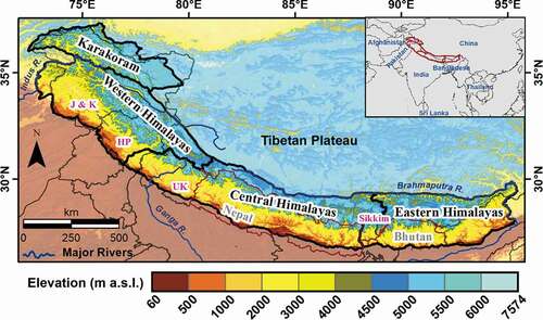
The KH region lies between 26.7 and 37.3°N and between 72.4 and 95.5°E, in the Hindu-Kush Himalayan region. Primarily, it is recognized as the most significant frozen reservoir of freshwater in the form of perennial snow cover and glacier ice outside the polar regions. Consequently, the water availability in these regions substantially influences the upstream and downstream livelihood. The KH region includes 20 812 glaciers, which cover 37 824 km² area out of the total area of ~713 907 km² (Cogley 2011). This region comprises parts of India, Pakistan, Nepal, Bhutan, and China, and contains many of the tallest mountain systems in the world.

Based on the climate and geographic location, the region is divided into four parts, i.e. the Karakoram (KK), Western (WH), Central (CH), and Eastern Himalayas (EH), covering an area of 56 487, 210 389, 280 635, and 166 397 km², respectively, previously expressed by Bolch et al. (2012) (Fig. 1). These regions are characterized based on their terrain properties and global atmospheric circulation pattern. Moreover, the areas are primarily nourished by two sources of precipitation, the Mid-Latitude Westerlies (MLW) and the Indian Summer Monsoon (ISM). The MLW precipitation greatly influences the KK and WH regions during the winter and spring seasons, accounting for ~60–70% of the total precipitation annually (Shrestha et al. 2015). In comparison, the ISM has a higher impact on the EH and CH region during the summer. The monsoonal precipitation decreases while moving from the east (∼1071 mm annual precipitation in the Brahmaputra basin) to the west (∼423 mm in the Indus basin) in the Himalayan region (Immerzeel et al. 2010). Changes in these two precipitation regimes with respect to intensity and frequency cause serious concern regarding the water resources of the downstream region.

Figure 1. Location map of the Karakoram and Himalayan (KH) region showing major rivers and altitude variation using Global Digital Elevation Model (GDEM) of Shuttle Radar Topography Mission (SRTM) v. 3.0 at 90-m grid resolution along the region. Abbreviations stand for Jammu & Kashmir (J&K), Himachal Pradesh (HP), and Uttarakhand (UK)

3 Materials and methods

3.1 Data used

3.1.1 MODIS snow cover products

This study utilizes the daily MODIS snow cover products of Terra (MOD10A1) and Aqua (MYD10A1) level-3 global version 6 (V6) over the KH region from 1 October 2000 to 30 September 2019 (19 hydrological years) (Riggs et al. 2016). The latest version of the MODIS products (V6) was used instead of the previous version 5 (V5). Zhang et al. (2019) found that V6 products have higher accuracy than V5. These snow products are freely available from the National Aeronautics and Space Administration (NASA) with 500-m grid resolution on the Earth data gateway customizable service (https://search.earthdata.nasa.gov).

Daily snow products are retrieved using the snow cover detection algorithm, beginning with the MOD10_L2 and MYD10L2 products in the MODIS snow product series (Riggs et al. 2016). The snow cover map of each product was reclassified into three new classes, 1 (i.e. snow cover conditions), 0 (i.e. snow-free conditions), and 2 (i.e. missing land information conditions). For snow, if the Normalized Difference Snow Index (NDSI) percentage value is greater than 40 and less than or equal to 100, then the land pixel is reclassified as “snow or 1.” When the NDSI value is greater than or equal to 0 and less than or equal to 40, or represents inland water, the pixel value is treated as “no-snow or 0.” The rest of the pixels were considered “cloud or 2.” Here, we have used an NDSI value greater than 40%, as suggested for snow cover mapping (Riggs et al. 2017).

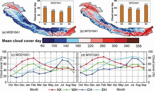
The KH region covers a total of 14 MODIS tiles, with numbers h22v05, h22v06, h23v05, h23v06, h24v05, h24v06, h25v05, h25v06, h26v05, h26v06, h27v05, h27v06, h28v05, and h28v06. This study utilized the Terra data from 1 October 2000 to 30 September 2019 and Aqua data from 4 July 2002 to 30 September 2019. A few images were found to be missing in both the products during the study period; therefore, the data gaps were replaced by their corresponding MODIS images (i.e. Terra images were replaced by Aqua images or vice versa). We have assumed that the missing images of the non-Aqua period (in Terra) were replaced by 100% cloud-covered images. The spatio-temporal distribution of cloud cover in MODIS products was mapped (Fig. 2), illustrating a higher cloud cover percentage in Aqua as compared to Terra of the total geographical area. The cloud cover percentage varied from region to region; the minimum value was observed in CH, and the maximum value was observed in EH.

Figure 2. Comparison between spatial mean cloud cover day of (a) MOD10A1 (from 1 October 2000 to 30 September 2019) and (b) MYD10A1 (from 1 October 2002 to 30 September 2019) along with temporal mean monthly cloud cover percentage of the total geographical area of (c) MOD10A1 and (d) MYD10A1 products in different sub-regions of the Karakoram and Himalayas (KH). KK: Karakoram; WH: Western Himalayas; CH: Central Himalayas; EH: Eastern Himalayas

3.1.2 Landsat 8-OLI data

To assess the reliability of the cloud-gap-filled MODIS snow product, we utilized the Landsat-8 Operational Land Imager (OLI) data between 2015 and 2016. Several researchers have already used the Landsat data to validate the MODIS dataset where the ground observations are rare (Hasson et al. 2014a, Tran et al. 2019). For this, 19 cloud-free images were selected with less than 5% cloud cover from the United States Geological Survey (USGS) EarthExplorer (http://earthexplorer.usgs.gov/) with a spatial and temporal resolution of 30 m and 16 days, respectively (Table 1).

Table 1. Description of the selected Landsat-8 OLI data for validating the cloud-filled MODIS SCA from 2015 to 2016 over the Karakoram and Himalayan (KH) region

Region	Row	Path	Date
Karakoram (KK)	149	035	31 October 2015, 2 December 2015, 19 January 2016, 10 May 2016
Western Himalaya (WH)	147	038	1 October 2015, 4 December 2015, 22 February 2016, 26 April 2016, 12 May 2016, 3 October 2016, 19 October 2016
Central Himalaya (CH)	142	040	1 December 2015, 17 December 2015, 3 February 2016, 22 March 2016
Eastern Himalaya (EH)	139	041	28 December 2015, 14 February 2016, 17 March 2016, 21 October 2016

3.1.3 MODIS Land Surface Temperature (LST) products

The standard monthly LST of MOD11C3 (Terra) and MYD11C3 (Aqua) products level-3 version 6 (V6) were utilized with a spatial resolution of 0.05° × 0.05° during 2000–2019 (19 hydrological years) for assessing the impact of surface temperature ($T_S$) on SCA variation. The data can be downloaded from https://search.earthdata.nasa.gov. The monthly LST values were retrieved from the average of four LST images (i.e. two images for Terra and two for Aqua, both day and night) of the corresponding month. Wan (2014) found that V6 LST products are much better than the previous V5.

3.1.4 NOAH Land Surface Model (LSM) data

The NOAH LSM level-4 monthly version 2.1 is a NASA Global Land Data Assimilation System (GLDAS) (Rodell et al. 2004) data product available at a grid resolution of 0.25° × 0.25° from 2000 to the present. It provides a consistent view of surface energy and water balance at the surface level from the past several decades (Rui and Beaudoing 2018). It is forced with a combination of model and observation data (Beaudoing and Rodell 2020). In this study, data on monthly relative humidity (RH), wind speed ($u$), albedo, sensible heat ($H_s$), latent heat ($H_l$), ground heat flux ($H_g$), net shortwave radiation (SWN), and net longwave radiation (LWN) were acquired between October 2000 and September 2019 to identify the changing pattern of these variables over the KH region. Data were retrieved from https://search.earthdata.nasa.gov.

3.1.5 ERA-5 data

ERA5 is a fifth-generation European Centre for Medium-Range Weather Forecasts (ECMWF) re-analysis (ERA-5) global climate and weather data, currently available from 1950 onwards and split into two separate periods in Climate Data Store entries, i.e. 1950–1978 and 1979 onwards, at a grid resolution of 0.25° × 0.25° with an hourly and monthly time scale (ECMWF 2019). ERA5 shows many improvements over the ERA-Interim reanalysis (Hoffmann et al. 2019), and it is also better than the other reanalysis products, as demonstrated in a study carried out by Mahto and Mishra (2019) over India. In this study, long-term monthly total precipitation ($P_t$) and air temperature ($T_a$) were acquired to quantify the trend of these variables over the KH region in two separate hydrological periods, i.e. 1979–2019 and 2000–2019. The data can be downloaded from https://cds.climate.copernicus.eu/cdsapp#!/dataset/reanalysis-era5-pressure-levels-monthly-means?tab=form.

3.1.6 In situ observation data

Daily climatic variables, i.e. air temperature (maximum and minimum) and snowfall, were used to analyse the relationships between MODIS snow cover and in situ data from 1 January 2013 to 31 December 2016. The data were obtained from the Snow and Avalanche Study Establishment (SASE), Chandigarh, India, at Patsio Observatory, located at 3800 m a.s.l. The site is characterized by a dry atmosphere with relatively low precipitation and cold temperature (Sharma and Ganju 2000).

3.1.7 Topographic data

The Global Digital Elevation Model (GDEM), version 3.0, was acquired from the Shuttle Radar Topography Mission (SRTM) at 90-m spatial resolution (Jarvis et al. 2008) to assess the influence of topographical parameters (i.e. elevation, aspect, and slope) on SCA variation. The DEM was resampled at a 500-m resolution using the bilinear interpolation technique (Lopez-Burgos et al. 2013) to match the spatial resolution of MODIS products.

3.2 Methodology

3.2.1 Composite methodology for cloud removal

A composite methodology for cloud-gap-filling in the MODIS snow cover products, that incorporates methods with accuracy >90%, was introduced and applied by numerous authors for cloud block removal (Gafurov and Bárdossy 2009, Parajka et al. 2010, Paudel and Andersen 2011, Hasson et al. 2014a, Wang et al. 2014, Jing et al. 2019, Tran et al. 2019). A five-step sequential non-spectral methodology was applied to mitigate the cloud gap in the MODIS snow products. The significance of using this composite methodology is that it includes all the necessary information about snow cover formation.

The first step includes merging twin satellite (Terra and Aqua) snow cover by assuming no snowfall or snowmelt occurred for a ~3–4 hour time difference at the Equator. Therefore, as long as a satellite captured (treated Terra as a base image) a pixel as snow or no-snow, then the cloud pixel will be replaced by the corresponding cloud-free pixel of the Aqua image. The equation for this is as follows

where $M_{\left(x,y,t\right)}^T$ and $M_{\left(x,y,t\right)}^A$are the Terra and Aqua images, respectively; $M_{\left(x,y,t\right)}^{CB}$ is the combined product (Terra and Aqua); and $\left(x,y,t\right)$ represents the spatial location $\left(x,y\right)$ of the present $\left(t\right)$ image.

In the second step, the present-day cloud pixel was assigned as snow (or no-snow), if the preceding and succeeding two days of images were acquired as pixels of snow (or no-snow). The equation for the given method is as follows:

where $M_{\left(x,y,t+1\right)}^{CB}$ and $M_{\left(x,y,t-1\right)}^{CB}$ shows the first day forward and backward from the image, respectively, and $M_{\left(x,y,t\right)}^{AD}$ is an adjacent temporal image. A similar logic was applied for t + 1 and t − 2 as well as t + 2 and t − 1 images.

The third step assigned the cloud grid as snow or no-snow based on the eight nearest neighbouring pixels and their topographical information (altitude and aspect) of the surrounding pixel. For this, a 3 × 3 moving window of two sequential iteration processes was considered for spatial filtering. In the first iteration, the cloud pixel is assigned as snow when any of the surrounding eight neighbouring pixels were captured as snow by satellite, and their elevation is less than the cloudy pixel with the same aspect. In contrast, if five out of eight cloud neighbouring pixels are snow/no-snow and cloud elevation is higher/lower than the elevation of minimum/maximum adjacent snow/no-snow pixel, then the cloud pixel is assigned as snow/no-snow in the second iteration. The final generated product of this step is defined as $M_{\left(x,y,t\right)}^{NN}$.

In the fourth method, the snowline/no-snowline threshold is utilized to classify the cloud pixel correctly. For this, the primary condition was that the present image must have at least 70% cloud-free pixels; otherwise, the method will be skipped. If the elevation of a cloud pixel was higher than the threshold, then the pixel was assigned as snow; otherwise, it was considered no-snow when it was below the threshold of the particular region. The final product of this step was denoted as $M_{\left(x,y,t\right)}^{SL}$.

In the last method, the remaining cloud grid pixel was eliminated by multiday backward replacement images. The primary assumption for this method was that there is no snowmelt or snowfall in the present-day image. The current-day cloud pixel was filled with the preceding day’s cloud-free pixels, and this continued until all the clouds in the image were removed. When the ground pixel has continuous cloud persistence, the cloud grid was assigned as a cloud, which enhances the uncertainty of that particular pixel. The method is explained by the following equation:

$\begin{array}{rl}& If(M_{\left(x,y,t\right)}^{SL}=cloud)=if(M_{\left(x,y,t-K\right)}^{SL}=snoworno-snow);\\ & then{M}_{\left(x,y,t\right)}^F=snoworno-snow\end{array}$

where $M_{\left(x,y,t\right)}^F$ indicates the final product of the applied methodology. K is the multiday previous day image or iteration of the approach (K = 1, 2, 3 …). Overall, the sequence and importance of the adopted methodology were explained by Dharpure et al. (2020) over the Chenab basin and validated with direct and indirect methods.

3.2.2 Accuracy assessment and validation

The validation of the cloud-gap-filled methodology is commonly carried out using ground truth data; however, this region has limited continuous records and scarce measurement locations and covers a broad geographical area. Therefore, the composite methodology was validated with the high-resolution satellite data and measured climatic data (snowfall and temperature).

In the first method, a total of 19 Landsat-8 images were utilized for area-based comparison with cloud-gap-filled MODIS images between 2015 and 2016. The Landsat-obtained snow cover was classified into a binary map based on the information acquired from reflectance bands (band 3 and 6). An NDSI [(band3-band6)/(band3+ band6)] threshold of >40% and near-infrared (reflectance band 5) >11% were considered for generating the binary snow cover map. The overlap region in each dataset was extracted and compared based on the relative error ($MODI{S}_{SCA}-Landsa{t}_{SCA}$) and mean absolute difference (MAD) [${\sum }^{a}bs\left(MODI{S}_{SCA}-Landsa{t}_{SCA}\right)/\mathrm{n}\mathrm{u}\mathrm{m}\mathrm{b}\mathrm{e}\mathrm{r}\mathrm{o}\mathrm{f}\mathrm{i}\mathrm{m}\mathrm{a}\mathrm{g}\mathrm{e}\mathrm{s}$]. For the second approach, the in situ measured monthly snowfall and mean air temperature were used to relate the MODIS SCA percentage over the Patsio Observatory (western Himalayas) from 1 January 2013 to 31 December 2016. For MODIS SCA estimation, a 5-km buffer zone was generated over the same location.

3.2.3 Snow cover indices

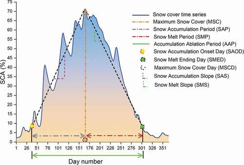
To understand the inter-annual variation, the SCD and nine other snow cover timing indices (derived from daily snow cover time series) were estimated during 2000–2019. The time series curve was extracted by plotting the daily SCA from 1 September to 31 August (Fig. 3), which can be used to characterize snow cover, previously applied by Dariane et al. (2017). In the KH, 19 snow cover time series curves (for each hydrological year) were obtained with a five-day moving average for removing the short-term variation in SCA. A brief description of each index is given below:

1. Snow accumulation onset day (SAOD) and snow melt ending day (SMED): The SAOD is the day when the snow accumulation started, and SMED is the day when the pixel is no longer covered by snow. For this, we have estimated a 25^th percentile value of daily SCA for each region, i.e. 36.9%, 9.4%, 5.4%, and 5.9% for the KK, WH, CH, and EH region, respectively, during the observational period. If the daily SCA is above the 25^th percentile value and remained continuous for the period, that particular date is denoted as SAOD, whereas if the SCA falls below the 25^th percentile value for the region, then the date is known as SMED. The changes in SAOD and SMED between years are mainly due to variation in precipitation, temperature, and solar radiation. The difference between SAOD and SMED is denoted as the accumulation–ablation period (AAP).

2. Maximum snow cover (MSC) and its day (MSCD): The maximum snow cover observed in each hydrological year is defined as MSC, and the day on which MSC occurred is denoted the MSCD. These indices are used to quantify the highest snow cover over the study area in a particular year.

3. Snow accumulation period (SAP) and snow melt period (SMP): SAP is a period between the day of snow accumulation onset and maximum snow cover, while the difference between the day of maximum snow cover and the melting end day is considered the SMP.

4. Snow accumulation slope (SAS) and snow melt slope (SMS): The rates of snow cover accumulation and melt are computed as MSC divided by the SAP and SMP during each hydrological year, respectively.

Figure 3. Pictorial representation of the snow cover time series and derived snow indices based on daily SCA in the western Himalayas (WH) from 1 September 2001 (Day 1) to 31 August 2002 (Day 366)

3.2.4 Statistical analysis

The spatio-temporal trends were analysed using the non-parametric Sen’s slope (Sen 1968) and Mann-Kendall (MK) (Mann 1945) trend test for the SCD, snow cover-derived indices, climatic and energy fluxes over seasonal, semi-annual, and annual scales at a 95% confidence interval. Pearson’s correlation coefficient (R) was also used to analyse the interrelationships of all variables. Additionally, the performance of estimated cloud-free MODIS SCA relative to Landsat-8 OLI was analysed based on bias [$(MODI{S}_{SCA}-Landsa{t}_{SCA})\times 100/Landsa{t}_{SCA}$] and root mean square error (RMSE). The annual relative change ratio (RCR in %) [(slope/mean) × number of years × 100] was estimated based on slope and mean SCA values during the study period (Baniya et al. 2018).

3.2.5 Sensitivity analysis

The sensitivity of SCA to climatic variables and energy fluxes was examined to determine the response of snow cover change with a potential indicator. The choices of these variables were based on the key properties of snowpack related to the snow cover onset timing and the amount of accumulated snow. To analyse the sensitivity of climatic variables ($T_a$ and $P_t$) and energy fluxes (SWN, LWN, $H_s$, and $H_l$) on SCA, we first standardized $\left(\left[\frac{value-mean}{standarddeviation}\right]\right)$ all the selected variables, and then generated a multivariant linear regression model over the sub-regions of KH.

4 Results

4.1 Validation of cloud-gap-filled MODIS snow products

To test the performance of the composite methodology, we used a two-step approach to validate the cloud-gap-filled SCA against high-resolution satellite data as well as meteorological data. In the first approach, 19 cloud-free Landsat-8 images were selected at different locations of the KH region and used to validate the area-based comparison between Landsat-8 and cloud-free MODIS SCA for the period 2015–2016. The results demonstrated that the MODIS SCA was highly correlated (R = 0.98, p < .001) with the Landsat-8 under the clear sky condition (Fig. 4(a)). The MAD between these two datasets was ~5.5%, while the relative error varied from 0.9 to 20.8. However, MODIS SCA was overestimated compared to Landsat-8.

Figure 4. (a) Comparison between MODIS SCA and Landsat-8 snow cover and (b) relationship of mean monthly SCA with in situ snowfall and air temperature over the Patsio observatory, western Himalayas

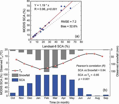
The second approach was carried out by establishing a relationship between cloud-free SCA and in situ observations (snowfall and air temperature) from 1 January 2013 to 31 December 2016 (Fig. 4(b)). The results demonstrate that the mean monthly SCA and snowfall were highly correlated (R = 0.84, p < .001). The in situ measured snowfall was maximum in February and minimum in August. This snowfall pattern may have been caused by the influence of westerlies in the Patsio location (WH), which receives higher snowfall in the winter months (December to April). On the other hand, the observed air temperature shows a significant negative correlation (R = −0.85, p < .001) with SCA. The lowest temperature was observed in January, while the highest was in July, followed by August over the Patsio location.

4.2 Snow cover variability

The accuracy of the composite methodology for cloud-gap-filling was evaluated and suggests that the estimated SCA was well matched with satellite as well as meteorological data. After analysing the performance of obtained results, we present the snow cover distribution at monthly, seasonal and annual scales, derived from daily cloud-gap-filled SCA over the KH region from 1 October 2000 to 30 September 2019. The monthly snow cover distribution exhibited a large heterogeneity in temporal scale over the region (Fig. 5), with higher SCA mainly concentrated in the KK and reduced SCA in the EH (see Supplementary material, Fig. S1). The snow accumulation started from October onwards and reached its maximum in February for KK, WH, and CH and in March for the EH region. The melting of snow starts from June onwards with the gradual rise in temperature, and snow cover attained maximum ablation in August. The minimum SCA was observed in August for KK and WH and in July and June for the CH and EH regions. Apart from this, the regions with the earliest snow accumulation onset eventually become the latest areas to melt off. Therefore, there is still scattered snow cover in July and August for the higher mountain areas, particularly the glacier accumulation region of the KH. The results also indicate that the variability of SCA was higher from October to December over the entire region and increased from KK to the EH region with a coefficient of variation (CV) of 13.3% and 55.6%, respectively.

Figure 5. Time series of monthly and yearly SCA in percentage over the (a) Karakoram (KK), (b) Western Himalayas (WH), (c) Central Himalayas (CH), and (d) Eastern Himalayas (EH). The bar graph illustrates the mean monthly SCA trends (nonsignificant at p < .05) for the period 2000–2019

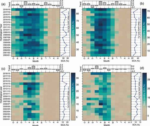
The mean monthly SCA trend of the KK increased for all months except in December, May, August, and September during the observation period (Fig. 5(a)). Similarly, the WH region showed an increasing monthly trend in SCA throughout the months except for December and January (Fig. 5(b)), and the CH region experienced an increasing SCA trend in all months except September to November (Fig. 5(c)). In the EH region, the mean monthly SCA shows a declining trend for all months, except for a slightly increasing trend from December to March (Fig. 5(d)). Overall, the mean monthly SCA shows an increasing trend in the accumulation months (February and March) while decreasing in the ablation months (August and September) in all regions.

The mean annual SCA distribution over the sub-regions of KH was determined, indicating that the KK region shows maximum SCA in 2004/2005 and minimum in 2000/2001 (Fig. 5(a)). In contrast, the WH received maximum and minimum annual SCA in 2018/2019 and 2000/2001, respectively (Fig. 5(b)). The CH attained its maximum mean annual SCA in 2014/2015 and minimum in 2015/2016 (Fig. 5(c)). In the EH region, the minimum and maximum SCA were observed at the start (2000/2001) and end (2018/2019), respectively, of the observational period (Fig. 5(d)). Further, the overall mean annual SCA trend was increasing over the KK, WH, and CH with a rate of 0.05, 0.11, and 0.02% year⁻¹, respectively, whereas a decreasing trend (–0.06% year⁻¹) was observed in the EH region during the study period; however, none of these trends were significant at p < .05. Overall, the KK and WH regions follow a similar pattern for SCA over the observational period, whereas the distribution of SCA in the CH region was qualitatively similar to the pattern of the EH region.

To examine the heterogeneity in SCA, we divided the whole hydrological period into two parts, i.e. 2000–2008 and 2008–2018. The year 2018/2019 was not considered because it was an exceptional year, according to Randhawa and Gautam (2019). The distribution of SCA and its trend over these two separate periods were evaluated and compared with the whole study period (2000–2019) (Table 2). The mean annual SCA from 2000 to 2019 shows an almost identical increasing trend from 2000 to 2008, except in the EH region. However, a decreasing trend of SCA was observed since 2008/2009 in all regions, with a maximum in the WH, which is statistically significant at p < .05, and a minimum in the CH (not significant). Additionally, the RCR shows the highest change in the WH and lowest in the KK region during 2008–2018. The RCR of SCA in the WH was the opposite in 2008–2018 compared to 2000–2008.

Table 2. Mean annual SCA and non-parametric Sen’s slope and Mann-Kendall (MK) trend test with relative change ratio (RCR in %) of SCA in three different hydrological periods over the Karakoram and Himalayan (KH) region and its sub-regions. The bold formatting indicates a significance level at p < .05

	Karakoram (KK)	Western Himalaya (WH)	Central Himalaya (CH)	Eastern Himalaya (EH)	Karakoram-Himalayas (KH)
2000–2019
Mean	52.4	30.5	12.6	10.2	26.4
Sen’s slope	0.05	0.11	0.02	−0.06	−0.00
RCR	1.63	7.16	3.64	−10.72	−0.18
2000–2008
Mean	52.4	30.0	12.3	10.6	26.3
Sen’s slope	0.11	0.68	0.04	0.33	0.21
RCR	1.93	20.37	3.07	27.79	7.23
2008–2018
Mean	52.4	30.6	12.4	9.7	26.3
Sen’s slope	−0.44	−0.80	−0.13	−0.24	−0.42
RCR	−8.37	−26.30	−10.84	−24.32	−16.06

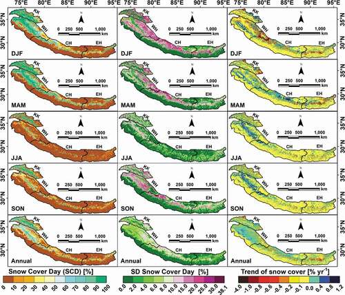
Pixel-wise mean monthly and annual SCD, and their standard deviation (SD), were derived for each hydrological year across the KH region (Fig. 6). The mean and SD attain minimum and maximum values in June, July, and August (JJA) and December, January, and February (DJF), respectively. The mean monthly spatial distribution of SCD was evaluated over the KH region (see Supplementary material, Fig. S2). The SD in the inter-annual variation of SCD displays a heterogeneous pattern similar to the spatially distributed mean, with relatively larger values in the KK and WH. A positive trend of SCD was observed in the KK, WH, and some locations of the CH region, whereas a negative trend was found in the EH region. This increasing trend indicates that the SCD was widened over the observation period for the KK and WH. Our results demonstrate that most of the area has come under no-SCD change, which indicates that SCD neither widened nor shortened for that region.

Figure 6. Mean seasonal and annual snow cover day (SCD) (left), standard deviation (SD) (middle), and SCD trend (right) over the Karakoram and Himalayan (KH) region from 2000 to 2019 hydrological year

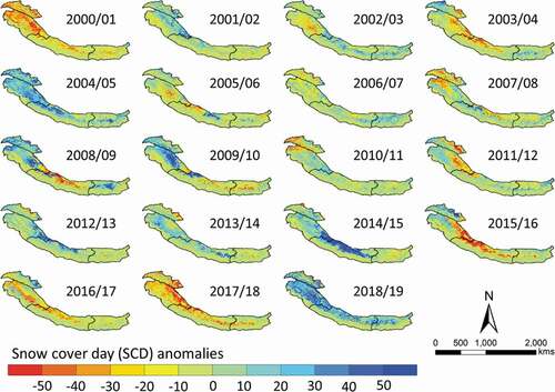
SCD anomalies play a significant role in global-scale atmospheric circulation over seasonal to annual scales. Therefore, we calculated the inter-annual SCD anomalies for each hydrological year from 2000 to 2019, indicating a more positive value in 2018/2019 and a negative value in 2017/2018 (Fig. 7). The upper reaches of the CH region experienced higher positive values (>50 days) in 2014/2015 and negative values in 2015/2016. Moreover, the year-to-year SCD variation in the KK was almost positive or stable from 2000–2019 except for 2000/2001, 2006/2008, 2010/2012, and 2017/2018. These positive anomalies in the KK suggest that the number of consecutive wet days increased over time.

Figure 7. Spatial patterns of annual snow cover day (SCD) anomalies during 2000–2019 over the Karakoram and Himalaya (KH) region were obtained by subtracting long-term annual SCD mean from individual hydrological year SCD

4.3 Snow cover metrics

In addition to SCD, nine other snow cover timing indices were mapped in each hydrological year through a five-day moving average of daily SCA over the sub-regions of KH to comprehend the properties of snow accumulation and melt period (Table 3). The results highlighted that the SAOD was shifted later by about one day per year in each region, and the mean onset day was about 4, 6, 12, and 20 October for KK, WH, CH, and EH, respectively, during 2000–2019. The MSC shows an increasing trend in all the regions except in the CH, and its mean value was decreasing from KK to the EH region. The MSCD shifted forward for the KK, WH, and EH at an average rate of one day per year. In comparison, the MSCD moved backward with an approximate trend of two days per year in the CH. The SAS shows a positive trend over the KK and WH, and a negative trend for the CH and EH. The SAP was narrowed for KK, WH, and EH, while it widened for CH. Furthermore, the SMP increased for KK and WH while it decreased for CH and EH. In contrast, the SMS also decreased, by an amount of −0.003 per year, in the WH. The SMED shows a mean snowmelt season end one day prior in each year over the EH, while it was delayed by one day in the other regions. In contrast, the AAP was widened over KK and WH and shortened for CH and EH.

Table 3. Sen’s slope and the mean value of derived snow timing indices in each sub-region of the Karakoram and Himalayas (KH) during 2000–2019. All trend slopes are not significant at p < .05

Region	KK	WH	CH	EH	KK	WH	CH	EH
Indices	Trend (Sen’s slope)				Mean annual
SAOD	0.31	0.64	1.40	0.33	34 (4 October)	36 (6 October)	42 (12 October)	50 (20 October)
MSC	0.13	0.12	–0.06	0.30	81.6	69.2	35.6	26.6
MSCD	–0.32	–0.12	1.67	–0.64	165 (12 February)	164 (11 February)	168 (15 February)	159 (6 February)
SMED	0.58	0.88	0.80	–0.76	300 (27 June)	304 (1 July)	285 (12 June)	273 (31 May)
AAP	0.50	0.60	–0.65	–0.90	266	269	243	223
SAP	–0.63	–0.67	0.45	–0.62	131	129	127	109
SMP	0.87	1.00	–1.10	–0.25	135	140	117	114
SAS	0.005	0.005	–0.004	0.002	0.78	0.56	0.32	0.28
SMS	–0.011	–0.003	0.001	0.004	0.66	0.50	0.32	0.25

4.4 Influence of meteorological variables on SCA

4.4.1 Long-term air temperature and precipitation variation (1979–2019)

To examine the long-term climatic variability and its trend over the region, we analysed $T_a$ and $P_t$ during hydrological years 1979–2019. This long-term analysis will help to determine a relationship between the short-term and long-term responses of the forcing variables. The temporal trend analysis of these variables was performed using linear regression, demonstrating that the $P_t$ slope indicates a declining trend in all regions except CH, whereas $T_a$ shows an increasing trend for the whole KH region (see Supplementary material, Fig. S3). 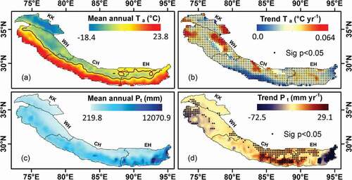Apart from this, the spatial distributions of $T_a$ and $P_t$ and their trends were quantified using Sen’s slope and the MK trend test over the region (Fig. 8). The mean annual $T_a$ was highlighted by the 0°C isotherm that separated temperatures above and below 0°C (Fig. 8(a)). The highest $P_t$ was found on the eastern side of the KH region, with an overall significant decreasing trend (Fig. 8(c)). A hotspot region in the WH was identified that indicates a significant decreasing trend of $P_t$, whereas an increasing trend was found for $T_a$. The results also demonstrate that the trend of $T_a$ was significantly increasing over the whole KH region, with a higher positive value in the eastern KK and western and northern WH, and a slightly lower positive value in the lower reaches of CH. Additionally, a small pocket of increasing $P_t$ trend was found over the lower portion of the CH region with a slightly less positive trend in $T_a$. Overall, this variability of long-term $T_a$ and $P_t$ helps in understanding the homogeneity and heterogeneity of climatic variables on SCA.

Figure 8. Spatio-temporal variation of mean yearly air temperature ($Ta$) and precipitation ($Pt$) with their trend (Sen’s slope) and trend significance level (black dot) over the Karakoram and Himalayan (KH) region from 1979 to 2019 (Source: https://cds.climate.copernicus.eu/cdsapp#!/dataset/reanalysis-era5-pressure-levels-monthly-means?tab=form)

4.4.2 Contribution of climatic variables and energy fluxes

The climatic variables ($T_a$, $T_S$, RH, $u$, albedo, and $P_t$), as well as energy fluxes (SWN, LWN, $H_s$, $H_l$, $H_g$, and net energy ($E_{net}$) fluxes) were examined from 2000 to 2019 to determine whether the variables showed any evidence of changes related to snow cover. The mean monthly variation of climatic variables (see Supplementary material, Fig. S4) and energy fluxes (see Supplementary material, Fig. S5) were assessed over the study area. The climatic variables suggest that the $T_a$ was directly proportional to the $T_S$ and RH, while it was inversely proportional to u and albedo. Other than that, the KK region experienced the highest seasonal variation in energy fluxes and the EH region had the lowest variability throughout the months.

The annual temporal (see Supplementary material, Fig. S6) and spatial (Fig. 9) trends of climatic variables and energy fluxes were assessed during 2000–2019. The results show a significant increasing trend of $T_a$,$T_S$, $P_t$, and $E_{net}$, while the other variables show a significantly decreasing trend at any particular location. The distribution of $P_t$ implies an increasing trend on the windward side of a mountain whereas it decreases on the leeward side of the mountain. Our results also indicate that the albedo and $P_t$ have a direct relationship with each other: when the albedo increases then $P_t$ also increases, and vice versa. Similarly, a significant decreasing trend of $u$ was observed over the selected region. Also, small pockets of SWN show an increasing trend; on the other hand, at the same location, the LWN was decreasing, which indicates that SWN and LWN have an inverse relationship with each other.

Figure 9. Spatial trend of climatic variables and energy fluxes over the Karakoram and Himalayan (KH) region from 2000 to 2019. The trend indicates Sen’s slope value, and black dots represent the significance level at p < .05

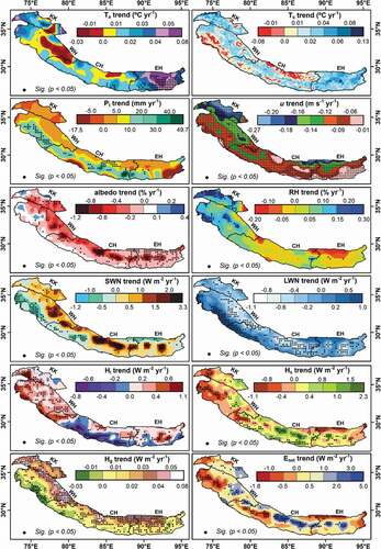
Moreover, the $E_{net}$ showed a positive trend in the eastern part of the KK region and a negative trend in the western region, which indicates less energy available for melt on the western side. The RH shows a decreasing trend in most CH and EH regions while increasing in the KK and some parts of CH. However, the higher SCA was mainly concentrated on the upper reaches (snow region) rather than in the lower reaches of KH, indicating the SWN, $H_l$, and $H_g$ were significantly increasing in the snowy region, which can contribute to SCA change. It was also noted that the variation of $P_t$ and LWN was higher (showing an increasing trend) in the no snow/little snow areas.

4.4.3 Relationships between SCA and climatic variables along with energy fluxes

Pearson’s correlation test was applied to establish the statistical relationships between mean annual SCA and climatic variables ($T_a$, $T_S$, $P_t$, RH and $u$) as well as energy fluxes (albedo, SWN, LWN,$R_N$,$H_l$, $H_S$, $H_g$ and $E_{net}$) over the KH region (Fig. 10). The results demonstrate that the SCA shows a strong positive correlation with albedo and a negative correlation with $T_a$ and $T_S$. Among the other climatic and heat flux variables, $P_t$ and RH were positively correlated with SCA over all regions, while $T_a$, $T_S$, SWN, $R_N$, $H_S$, and $E_{net}$ show an inverse relation over the KK, WH, and CH regions. In the EH region, almost all the essential climatic variables and energy fluxes showed a nonsignificant correlation with each other (except for the $T_a$). Moreover, in the EH region, the $T_s$ was negatively correlated with the $P_t$, RH, u, SWN, and LWN.

Figure 10. Relationships of SCA, climatic variables, and energy fluxes over the (a) Karakoram (KK), (b) Western Himalayas (WH), (c) Central Himalayas (CH), and (d) Eastern Himalayas (EH) for the period 2000–2019

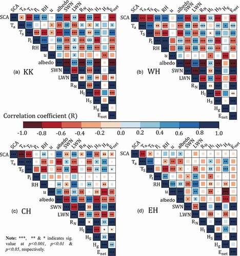
Similarly, the albedo was negatively correlated with the SWN, $R_N$, $H_S$, and $E_{net}$ over the selected regions. On the other hand, the positive correlation of $H_l$ with SCA was much stronger in the CH region. Overall, our results indicate that the decreasing pattern of SCA or the prolonged melting period significantly impacted the snow accumulation and decreased surface albedo, which can absorb higher solar radiation on the surface and vice versa. Therefore, the results suggest that the changing pattern of SCA is closely linked with these variables, while SCA characteristics varied from location to location.

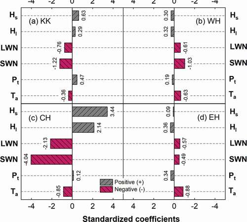
4.4.4 Sensitivity analysis of SCA

For the sensitivity analysis, the selected independent and dependent variables were standardized, and then multivariate linear regression models were generated at an annual time scale during 2000–2019 (Fig. 11). Our results suggest that the $T_a$ is a more significant climatic contributor than $P_t$ to SCA change for each region except KK. In the radiation components, SWN shows the largest proportion of the variance against LWN except for the EH region. Similarly, the $H_s$ showed higher sensitivity than $H_l$ over KK and CH, whereas in the WH and EH regions, the sensitivity of $H_l$ was higher relative to $H_s$. After analysing the strength of all the variables, statistics suggest that the whole KH region experienced higher sensitivity towards SWN, with the maximum in the CH region and the minimum in the EH region.

Figure 11. Sensitivity analysis of SCA in terms of climatic variables ($Ta$ and $Pt$) and energy fluxes (SWN, LWN, $Hl$, and $Hs$) over the (a) Karakoram (KK), (b) Western Himalayas (WH), (c) Central Himalayas (CH), and (d) Eastern Himalayas (EH)

5 Discussion

The spatio-temporal variation of SCA in the KH region is essential to understanding the land–atmosphere interaction and its implications for local water availability. This region is considered one of the more climate-sensitive regions across the world that directly or indirectly influences the livelihoods of millions of people (Choudhury et al. 2021). The monitoring of SCA in the KH region is mainly hindered by the limited availability of continuous in situ records and by cloud obstruction in the optical remote sensing data. The in situ-based constraint was resolved by the use of MODIS snow cover products that provide data at a larger spatial and fine temporal scale. The presence of clouds in the snow cover products was also managed, by implementing a five-step composite methodology. Several authors have previously developed and implemented this approach for cloud-gap-filling within the study region (Paudel and Andersen 2011, Hasson et al. 2014a) and its vicinity (Gafurov and Bárdossy 2009, Huang et al. 2017, Li et al. 2019). Our results on cloud-gap-filling showed higher accuracy with high-resolution satellite data as well as in situ observation. In this Himalayan context, many authors have used satellite and field observations to assess the performance of the cloud removal approach (Jain et al. 2008, Chelamallu et al. 2014, Muhammad and Thapa 2020). In our study, the comparison of MODIS products with Landsat data shows overestimation, consistent with the findings of prior studies (Tang et al. 2012, Hasson et al. 2014b, Muhammad and Thapa 2020).

Several inherent uncertainties in MODIS snow cover retrieval mainly occurred due to the larger solar zenith angles, which reduce the accuracy of the snow cover products (Li et al. 2016). On the other hand, the band consideration in Terra (band 6) and Aqua (band 7) for the NDSI calculation show higher accuracy in Terra than Aqua (Hall and Riggs 2007). Therefore, in the first step, the combination of Terra and Aqua can contribute some uncertainties in the cloud-gap-filling. Additionally, uncertainties are linked with the absolute validation of cloud-gap-filling snow cover products, that indicate ~90% accuracy under clear sky conditions (Klein and Barnett 2003, Hall and Riggs 2007). The correct estimation of snow cover under thick canopies is a major limitation of optical sensors (Simic et al. 2004). Still, this limitation was slightly reduced in the high mountainous region and glacier terrain. In these regions, the errors are likely to be highest in the transitional period (accumulation and ablation). Therefore, we have considered all-terrain information for reducing uncertainties in the region and enhancing the accuracy of the methodology.

The mean annual SCA trend was increasing for the entire region (KK, WH, and CH) except for the EH, during 2000–2019. Many authors have worked on basin- or local-scale SCA estimation, which shows a similar increasing trend over the KK region (Hasson et al. 2014a, Singh et al. 2014, Tahir et al. 2016, Bilal et al. 2019, Choudhury et al. 2021). This increasing trend of SCA might be the reason for positive mass balance in the glaciers of the Karakoram region, as illustrated by numerous authors (Gardelle et al. 2012, 2013, Mukhopadhyay and Khan 2014, Mukhopadhyay et al. 2015, Negi et al. 2020). Additionally, Farinotti et al. (2020) revealed that the KK glaciers were experiencing positive mass gain, and their terminus was even advancing due to the surging of the glacier.

Similarly, several authors have investigated the increasing snow cover pattern over the WH region at different spatial scales, i.e. regional (Zhang 2015, Tayal 2017, Sood et al. 2020, Choudhury et al. 2021), basin (Kulkarni et al. 2010, Snehmani et al. 2016, Dharpure et al. 2020) and local (Kour et al. 2016, Shafiq et al. 2018). On the other hand, some studies at a finer scale have documented decreasing SCA in the CH region (Paudel and Andersen 2011, Singh et al. 2014), which is not consistent with our findings; this may be due to the difference in spatial scale. Also, a decreasing SCA trend was observed over the EH, which was previously monitored and explained by several authors (Singh et al. 2014, Barman and Bhattacharjya 2015, Basnett and Kulkarni 2019, Maurer et al. 2019).

Our findings for the KK region not only illustrate the higher SCA but also indicate that the snow accumulation onset was shifted one day later with an increasing snow melting period. This indicates that the amount of snowfall was higher than the rate of melting; therefore, the region depicted mass gain or nearly stable conditions. Farinotti et al. (2020) observed that the KK region experienced an increased snowfall in the accumulation zone, with higher surface albedo and even a reduction in net energy available for the melt. Our findings for the WH region highlighted an increasing trend of snow accumulation onset time, whereas the snow melt period was enlarged during the study period. This may have occurred due to the higher snow melting rate under the influence of rising temperature in the WH region (Shekhar et al. 2010). In the CH and EH regions, the snow accumulation onset was shifted forward, whereas the snow accumulation period was positive for CH and negative for EH. In addition, the snow melting period was shortened for both CH and EH regions. Paudel and Andersen (2011) reported a peak snow period delayed by 6.7 days per year and peak snowfall over the Trans-Himalayan region of Nepal (CH) during 2000–2010. Panday et al. (2011) found that the late melt onset of the CH contributed to the shortening of the melt period in 2003 and 2005. They also demonstrated that the EH region in Nepal and Bhutan showed an earlier melt onset than the CH, WH, and KK regions.

Reliable quantification of forcing variables and their mechanisms is needed to understand the interaction of the atmosphere and microclimatic conditions with changing SCA. Therefore, we used climatic variables and energy fluxes over the KH region. The climatic variables show that the precipitation followed an increasing trend over the whole region during 2000–2019, with the maximum slope in CH and the minimum in KK, whereas the temperature trend of the KH region was significantly increasing. Our findings are consistent with previous studies over the KH region (Gautam et al. 2013, Sabin et al. 2020). This increasing trend of precipitation causes a significant increase in wet days and an increase in wintertime precipitation, which further results in increasing SCA. In contrast, the association of SCA with the radiative forcing variables illustrates that the SWN was the main contributor to the net energy available for melt. The higher SWN was observed in the CH, which is consistent with the findings of Amatya et al. (2015), whereas SWN was slightly lower in the KK region. Bonekamp et al. (2019) found that the melt in KK was controlled by the SWN while LWN dominates the energy balance in the Langtang region (CH). In terms of spatial variability, we found significant increasing trends of SWN, $H_l$, and $H_g$ in the snowy region whereas $P_t$ and LWN increased in the non-snowy region. This pattern was also noticed by some other authors (Amatya et al. 2015, Patel et al. 2021).

By combining it with the published literature, our results suggest a broad picture of snow cover variability. These records of snow cover change indicate that the majority of the SCA trend was increasing over the KH and its sub-regions (except for the EH region). Also, SCA increased where precipitation increased in the coldest region (KK), whereas it decreased where precipitation decreased in the warmest region (EH). A more detailed investigation in future research will be needed in the KH region, focusing on basin-wide SCA characterization and its modelling for streamflow prediction. This study would be helpful not only for continuous SCA monitoring but also for establishing the relationship of SCA with the direct or indirect dependent variables.

6 Conclusions

This study examined the spatio-temporal snow cover variability using daily MODIS cloud-gap-filled SCA over the KH region during 2000–2019. The results revealed that the maximum SCA was mainly concentrated on the KK region, while the minimum occurred in the EH region. The annual SCA trend was increasing for each region except for the EH, during 2000–2019, but these trends were not significant at p < .05; whereas it showed a significant declining trend over the entire region and its sub-regions for the period 2008–2018. The mean monthly SCA increased in the accumulation months (February and March) and decreased in the ablation months (August and September) over the region. The results also highlighted that the snow accumulation onset and melt periods were shifted one day later for all regions except the EH. Due to the shrinking of SCA, the flow of rivers originating from the KH region is likely to be reduced during the summer season, which may affect the socio-economic conditions at the higher altitudes in terms of vegetation cultivation, tourism, and apple farming.

In relation to this, the annual $T_a$ and $P_t$ trends were evaluated, which indicate an increasing trend of annual $P_t$ during 2000–2019 with a maximum slope in the CH region and a minimum slope in the KK region. The annual $T_a$ shows an increasing trend for the study period, with a higher rate in EH and a lower rate in WH. Our results also indicate that the temperature ($T_a$ and $T_s$) and $P_t$ from the selected climatic variables and SWN from radiative fluxes were mainly responsible for the changing pattern of SCA over the KH region. Overall, we conclude from this study that the SCA of the KH region is highly variable from location to location. Even the influence of climatic variables and energy fluxes related to SCA change may vary with the snowy or non-snowy region. Therefore, a reliable estimation of SCA and its relationship with these forcing variables will help to provide a better understanding of future water supply and its management in the upstream and downstream regions.

Acknowledgements

The authors are grateful to the anonymous reviewers and the Associate Editor (Dr Stephanie Kampf), whose comments and suggestions have significantly improved the manuscript. The authors also acknowledge the Indian Institute of Technology, Roorkee, India, for providing the necessary infrastructure facilities.

Data availability statement

Data available on request due to privacy/ethical restrictions.

Disclosure statement

No potential conflict of interest was reported by the author(s).

Supplementary material

Supplemental data for this article can be accessed here

Additional information

Funding

This article was funded by the National Centre for Polar and Ocean Research, Goa, India [grant agreement number NCAOR/ 2018/HiCOM/03/]; and the Indian Institute of Technology, Roorkee, India [Project No. MES-1193-DMC].

References

- Amatya, P.M., et al., 2015. Recent trends (2003–2013) of land surface heat fluxes on the southern side of the central Himalayas, Nepal. Journal of Geophysical Research: Atmospheres, 120 (11), 957–970. doi:https://doi.org/10.1002/2015JD023510.
- Baniya, B., et al., 2018. Spatial and temporal variation of NDVI in response to climate change and the implication for carbon dynamics in Nepal. Forests, 9 (6), 1–18. doi:https://doi.org/10.3390/f9060329.
- Barman, S. and Bhattacharjya, R.K., 2015. Change in snow cover area of Brahmaputra river basin and its sensitivity to temperature. Environmental Systems Research, 4 (1). Springer Berlin Heidelberg. doi:https://doi.org/10.1186/s40068-015-0043-0.
- Basnett, S. and Kulkarni, A.V., 2019. Snow cover changes observed over Sikkim Himalaya. A. Saikia and P. Thapa Eds. Cham: Springer International Publishing. Springer Nature Switzerland. doi:https://doi.org/10.1007/978-3-030-03362-0.
- Beaudoing, H.K., Rodell, M. and NASA/GSFC/HSL, 2020. LDAS NOAH land surface model L4 monthly 0.25 x 0.25 degree V2.1. Greenbelt, Maryland: Goddard Earth Sciences Data and Information Services Center (GES DISC). doi:https://doi.org/10.5067/SXAVCZFAQLNO.
- Bilal, H., et al., 2019. Recent snow cover variation in the upper Indus basin of Gilgit Baltistan, Hindukush Karakoram Himalaya. Journal of Mountain Science, 16 (2), 296–308. doi:https://doi.org/10.1007/s11629-018-5201-3.
- Bolch, T., et al., 2012. The state and fate of himalayan glaciers. Science (80-.), 336 (6079), 310–314. doi:https://doi.org/10.1126/science.1215828.
- Bonekamp, P.N.J., et al., June 2019. Contrasting meteorological drivers of the glacier mass balance between the Karakoram and central Himalaya. Frontiers in Earth Science, 7, 1–14. doi:https://doi.org/10.3389/feart.2019.00107.
- Chelamallu, H.P., Venkataraman, G., and Murti, M.V.R., 2014. Accuracy assessment of MODIS/Terra snow cover product for parts of Indian Himalayas. Geocarto International, 29 (6), 592–608. doi:https://doi.org/10.1080/10106049.2013.819041.
- Chen, S., et al., 2020. Spatial and temporal adaptive gap-filling method producing daily cloud-free NDSI time series. IEEE Journal of Selected Topics in Applied Earth Observations and Remote Sensing, 13, 2251–2263. doi:https://doi.org/10.1109/jstars.2020.2993037
- Choudhury, A., Yadav, A.C., and Bonafoni, S., 2021. A response of snow cover to the climate in the northwest himalaya (Nwh) using satellite products. Remote Sensing, 13 (4), 1–22. doi:https://doi.org/10.3390/rs13040655.
- Cogley, J.G., 2011. Present and future states of Himalaya and Karakoram glaciers. Annals of Glaciology, 52 (59), 69–73. doi:https://doi.org/10.3189/172756411799096277.
- Dankers, R. and De Jong, S.M., 2004. Monitoring snow-cover dynamics in Northern Fennoscandia with SPOT VEGETATION images. International Journal of Remote Sensing, 25 (15), 2933–2949. doi:https://doi.org/10.1080/01431160310001618374.
- Dariane, A.B., Khoramian, A., and Santi, E. 2017. Investigating spatiotemporal snow cover variability via cloud-free MODIS snow cover product in Central Alborz region. Remote Sensing of Environment, 202, 152–165. Elsevier Inc. doi:https://doi.org/10.1016/j.rse.2017.05.042.
- Dharpure, J.K., et al., 2020. Spatiotemporal snow cover characterization and its linkage with climate change over the Chenab river basin, western Himalayas. GIScience Remote Sensing, 1–25. Taylor & Francis. doi:https://doi.org/10.1080/15481603.2020.1821150.
- ECMWF, 2019. Essential climate variables for assessment of climate variability from 1979 to present. Copernicus Climate Change Service. 1–10.
- Farinotti, D., et al., 2020. Manifestations and mechanisms of the Karakoram glacier Anomaly. In: EGU General Assembly Conference Abstract, 13, 8–16. doi:https://doi.org/10.1038/s41561-019-0513-5.
- Foster, J.L., Chang, A.T., and Hall, D.K. 1995. Snow mass in boreal forests derived from a modified passive microwave algorithm. Satellite Remote Sensing, 2314, 605–617. International Society for Optics and Photonics.
- Gafurov, A., et al., 2015. Snow-cover reconstruction methodology for mountainous regions based on historic in situ observations and recent remote sensing data. The Cryosphere, 9 (2), 451–463. doi:https://doi.org/10.5194/tc-9-451-2015.
- Gafurov, A. and Bárdossy, A., 2009. Cloud removal methodology from MODIS snow cover product. Hydrology and Earth System Sciences, 13 (7), 1361–1373. doi:https://doi.org/10.5194/hess-13-1361-2009.
- Gao, Y., et al., 2010. Toward advanced daily cloud-free snow cover and snow water equivalent products from Terra–Aqua MODIS and Aqua AMSR-E measurements. Journal of Hydrology, 385 (1), 23–35. doi:https://doi.org/10.1016/j.jhydrol.2010.01.022.
- Gardelle, J., et al., 2013. Region-wide glacier mass balances over the Pamir-Karakoram-Himalaya during 1999-2011. Cryosphere, 7 (4), 1263–1286. doi:https://doi.org/10.5194/tc-7-1263-2013.
- Gardelle, J., Berthier, E., and Arnaud, Y., 2012. Slight mass gain of Karakoram glaciers in the early twenty-first century. Nature Geoscience, 5 (5), 1–4. Nature Publishing Group. doi:https://doi.org/10.1038/ngeo1450.
- Gautam, M.R., Timilsina, G.R., and Acharya, K., 2013. Climate change in the Himalayas: current state of knowledge. World Bank Development Research Group Environment and Energy Team. doi:https://doi.org/10.1596/1813-9450-6516.
- Gurung, D.R., et al., 2011. Snow-cover mapping and monitoring in The Hindu Kush-Himalayas. Kathmandu, Nepal: International Centre for Integrated Mountain Development (ICIMOD).
- Hall, D.K., Foster, J.L., and Chang, A.T.C., 1982. Measurement and modeling of microwave emission from forested snowfields in Michigan. Hydrology Research, 13 (3), 129–138. doi:https://doi.org/10.2166/nh.1982.0011.
- Hall, D.K. and Riggs, G.A., 2007. Accuracy assessment of the MODIS snow products. Hydrological Processes, 21 (12), 1534–1547. doi:https://doi.org/10.1002/hyp.6715.
- Hall, D.K., Riggs, G.A., and Salomonson, V.V., 1995. Mapping global snow cover using moderate resolution imaging spectroradiometer (MODIS) data. Remote Sensing of Environment, 54 (3), 127–140. doi:https://doi.org/10.1016/0034-4257(95)00137-P.
- Hasson, S., et al., 2014a. Early 21st century snow cover state over the western river basins of the Indus river system. Hydrology and Earth System Sciences, 18 (10), 4077–4100. doi:https://doi.org/10.5194/hess-18-4077-2014.
- Hasson, S., et al., 2014b. Seasonality of the hydrological cycle in major South and Southeast Asian river basins as simulated by PCMDI/CMIP3 experiments. Earth System Dynamics, 5 (1), 67–87. doi:https://doi.org/10.5194/esd-5-67-2014.
- Hoffmann, L., et al., 2019. From ERA-Interim to ERA5: the considerable impact of ECMWF’s next-generation reanalysis on Lagrangian transport simulations. Atmospheric Chemistry and Physics, 19 (5), 3097–3124. doi:https://doi.org/10.5194/acp-19-3097-2019.
- Huang, X., et al., 2014. A new MODIS daily cloud free snow cover mapping algorithm on the Tibetan Plateau. Sciences in Cold and Arid Regions, 6 (2), 0116–123. doi:https://doi.org/10.3724/SP.J.1226.2014.00116.
- Huang, X., et al. 2017. Impact of climate and elevation on snow cover using integrated remote sensing snow products in Tibetan Plateau. Remote Sensing of Environment, 190, 274–288. Elsevier Inc. doi:https://doi.org/10.1016/j.rse.2016.12.028.
- Immerzeel, W.W., Van Beek, L.P.H., and Bierkens, M.F.P., 2010. Climate change will affect the asian water towers. Science (80-.), 328 (5984), 1382–1385. doi:https://doi.org/10.1126/science.1183188.
- Jain, S.K., Goswami, A., and Saraf, A.K., 2008. Accuracy assessment of MODIS, NOAA and IRS data in snow cover mapping under Himalayan conditions. International Journal of Remote Sensing, 29 (20), 5863–5878. doi:https://doi.org/10.1080/01431160801908129.
- Jarvis, A., et al., 2008. Hole-filled SRTM for the globe version 4, from the CGIAR-CSI SRTM 90m database. Available from: http://srtm.csi.cgiar.org
- Jing, Y., et al., 2019. A two-stage fusion framework to generate a spatio’temporally continuous MODIS NDSI product over the Tibetan Plateau. Remote Sensing, 11 (19), 1–21. doi:https://doi.org/10.3390/rs11192261.
- Klein, A.G. and Barnett, A.C., 2003. Validation of daily MODIS snow cover maps of the upper Rio Grande river basin for the 2000–2001 snow year. Remote Sensing of Environment, 86 (2), 162–176. doi:https://doi.org/10.1016/S0034-4257(03)00097-X.
- Kour, R., Patel, N., and Krishna, A.P., 2016. Assessment of temporal dynamics of snow cover and its validation with hydro-meteorological data in parts of Chenab basin, western Himalayas. Science China Earth Sciences, 59 (5), 1081–1094. doi:https://doi.org/10.1007/s11430-015-5243-y.
- Kulkarni, A.V., et al., 2006. Algorithm to monitor snow cover using AWiFS data of RESOURCESAT-1 for the Himalayan region. International Journal of Remote Sensing, 27 (12), 2449–2457. doi:https://doi.org/10.1080/01431160500497820.
- Kulkarni, A.V., et al., 2010. Distribution of seasonal snow cover in central and western Himalaya. Annals of Glaciology, 51 (54), 123–128. doi:https://doi.org/10.3189/172756410791386445.
- Kulkarni, A.V., et al., 2011. Understanding changes in the Himalayan cryosphere using remote sensing techniques. International Journal of Remote Sensing, 32 (3), 601–615. doi:https://doi.org/10.1080/01431161.2010.517802.
- Kumar, M. and Kumar, P., 2016. Snow cover dynamics and geohazards: a case study of Bhilangna watershed, Uttarakhand Himalaya, India. Geoenvironmental Disasters, 3 (1), 0–7. Geoenvironmental Disasters. doi:https://doi.org/10.1186/s40677-016-0035-z.
- Li, H., Li, X., and Xiao, P., 2016. Impact of sensor zenith angle on MOD10A1 data reliability and modification of snow cover data for the Tarim river basin. Remote Sensing, 8 (9), 1–18. doi:https://doi.org/10.3390/rs8090750.
- Li, X., et al., 2017. Monitoring snow cover variability (2000–2014) in the Hengduan mountains based on cloud-removed MODIS products with an adaptive spatio-temporal weighted method. Journal of Hydrology, 551, 314–327. doi:https://doi.org/10.1016/j.jhydrol.2017.05.049
- Li, X., et al., 2019. The recent developments in cloud removal approaches of MODIS snow cover product. Hydrology and Earth System Sciences, 23 (5), 2401–2416. doi:https://doi.org/10.5194/hess-23-2401-2019.
- Li, Y., Chen, Y., and Li, Z., 2019. Developing daily cloud-free snow composite products from MODIS and IMS for the Tienshan mountains. Earth and Space Science, 6 (2), 266–275. doi:https://doi.org/10.1029/2018EA000460.
- Liang, T.G., et al., 2008. An application of MODIS data to snow cover monitoring in a pastoral area: a case study in Northern Xinjiang, China. Remote Sensing of Environment, 112 (4), 1514–1526. doi:https://doi.org/10.1016/j.rse.2007.06.001.
- Lopez-Burgos, V., Gupta, H.V., and Clark, M., 2013. Reducing cloud obscuration of MODIS snow cover area products by combining spatio-temporal techniques with a probability of snow approach. Hydrology and Earth System Sciences, 17 (5), 1809–1823. doi:https://doi.org/10.5194/hess-17-1809-2013.
- Mahto, S.S. and Mishra, V., 2019. Does ERA-5 outperform other reanalysis products for hydrologic applications in India? Journal of Geophysical Research: Atmospheres, 124 (16), 9423–9441. doi:https://doi.org/10.1029/2019JD031155.
- Mann, H.B., 1945. Nonparametric tests against trend. Econometrica, 13 (3), 245–259. doi:https://doi.org/10.1016/j.annrmp.2004.07.001.
- Maurer, J.M., et al., 2019. Acceleration of ice loss across the Himalayas over the past 40 years. Science Advances, 5 (6). doi:https://doi.org/10.1126/sciadv.aav7266.
- Muhammad, S. and Thapa, A., 2020. An improved Terra-Aqua MODIS snow cover and Randolph Glacier Inventory 6.0 combined product (MOYDGL06) for high-mountain Asia between 2002 and 2018. Earth System Science Data, 12 (1), 345–356. doi:https://doi.org/10.5194/essd-12-345-2020.
- Mukherji, A., et al., 2019. Contributions of the cryosphere to mountain communities in The Hindu Kush Himalaya: a review. Regional Environmental Change, 19 (5), 1311–1326. Regional Environmental Change. doi:https://doi.org/10.1007/s10113-019-01484-w.
- Mukhopadhyay, B., Khan, A., and Gautam, R., 2015. Rising and falling river flows: contrasting signals of climate change and glacier mass balance from the eastern and western Karakoram. Hydrological Sciences Journal, 60 (12), 2062–2085. Taylor & Francis. doi:https://doi.org/10.1080/02626667.2014.947291.
- Mukhopadhyay, B. and Khan, A. 2014. Rising river flows and glacial mass balance in central Karakoram. Journal of Hydrology, 513, 192–203. Elsevier B.V. doi:https://doi.org/10.1016/j.jhydrol.2014.03.042.
- Negi, H.S., et al. 2020. Status of glaciers and climate change of East Karakoram in early twenty-first century. Science of the Total Environment, 753, 141914. Elsevier B.V. doi:https://doi.org/10.1016/j.scitotenv.2020.141914.
- Negi, H.S., Kulkarni, A.V., and Semwal, B.S., 2009. Estimation of snow cover distribution in Beas basin, Indian Himalaya using satellite data and ground measurements. Journal of Earth System Science, 118 (5), 525–538. doi:https://doi.org/10.1007/s12040-009-0039-0.
- Panday, P.K., Frey, K.E., and Ghimire, B., 2011. Detection of the timing and duration of snowmelt in The Hindu Kush-Himalaya using QuikSCAT, 2000–2008. Environmental Research Letters, 6 (2), 2000–2008. doi:https://doi.org/10.1088/1748-9326/6/2/024007.
- Parajka, J., et al., 2010. A regional snow-line method for estimating snow cover from MODIS during cloud cover. Journal of Hydrology, 381 (3), 203–212. doi:https://doi.org/10.1016/j.jhydrol.2009.11.042.
- Parajka, J. and Blöschl, G., 2008. Spatio-temporal combination of MODIS images - potential for snow cover mapping. Water Resources Research, 44 (3). doi:https://doi.org/10.1029/2007WR006204.
- Patel, A., et al., 2021. Regional mass variations and its sensitivity to climate drivers over glaciers of Karakoram and Himalayas. GIScience Remote Sensing, 1–23. Taylor & Francis. doi:https://doi.org/10.1080/15481603.2021.1930730.
- Paudel, K.P. and Andersen, P., 2011. Monitoring snow cover variability in an agropastoral area in the Trans Himalayan region of Nepal using MODIS data with improved cloud removal methodology. Remote Sensing of Environment, 115 (5), 1234–1246. doi:https://doi.org/10.1016/j.rse.2011.01.006.
- Randhawa, S.S. and Gautam, N., 2019. Assessment of spatial distribution of seasonal snow cover during the year 2018–19 in Himachal Pradesh using space data. Available from: http://www.hpccc.gov.in/documents/SnowCoverAnalysis.pdf
- Riggs, G.A., Hall, D.K., and Roman, M.O., August 2016. MODIS snow products collection 6 user guide. Boulder, CO: National Snow and Ice Data Center, 6, 1–80. Available from: https://modis-snow-ice.gsfc.nasa.gov/uploads/C6_MODIS_Snow_User_Guide.pdf
- Riggs, G.A., Hall, D.K., and Román, M.O., 2017. Overview of NASA’s MODIS and Visible Infrared Imaging Radiometer Suite (VIIRS) snow-cover Earth system data records. Earth System Science Data, 9 (2), 765–777. doi:https://doi.org/10.5194/essd-9-765-2017.
- Rodell, M., et al., March 2004. The global land data assimilation system. Bulletin of the American Meteorological Society, 85 (3), 381–394. doi:https://doi.org/10.1175/BAMS-85-3-381.
- Rui, H. and Beaudoing, H.K. 2018. README document for GLDAS version 2 data products. Goddard Earth Sciences Data and Information Services Center (GES DISC), 1–32. Available from: http://hydro1.sci.gsfc.nasa.gov/data/s4pa/GLDAS/GLDAS_NOAH10_M.2.0/doc/README_GLDAS2.pdf
- Sabin, T.P., et al., 2020. Climate change over the Himalayas. In: R. Krishnan, et al., eds. Assessment of climate change over the Indian region: a report of the Ministry of Earth Sciences (MoES), Government of India. Singapore: Springer, 207–222. doi:https://doi.org/10.1007/978-981-15-4327-2_11.
- Sen, P.K., 1968. Estimates of the regression coefficient based on Kendall’s Tau. Journal of the American Statistical Association, 63 (324), 1379–1389. doi:https://doi.org/10.1080/01621459.1968.10480934.
- Shafiq, M.U., et al. 2018. Snow cover area change and its relations with climatic variability in Kashmir Himalayas, India. Geocarto International, 6049, 1–15. Taylor & Francis. doi:https://doi.org/10.1080/10106049.2018.1469675.
- Sharma, S.S. and Ganju, A., 2000. Complexities of avalanche forecasting in western Himalaya - an overview. Cold Regions Science and Technology, 31 (2), 95–102. doi:https://doi.org/10.1016/S0165-232X(99)00034-8.
- Shekhar, M.S., et al., 2010. Climate-change studies in the western Himalaya. Annals of Glaciology, 51 (54), 105–112. doi:https://doi.org/10.3189/172756410791386508.
- Shrestha, A., et al., 2015. The Himalayan climate and water atlas: impact of climate change on water resources in five of Asia’s major river basins. Nepal, Norway and Sweden: ICIMOD, GRID-Arendal and CICERO.
- Simic, A., et al., 2004. Validation of VEGETATION, MODIS, and GOES+ SSM/I snow‐cover products over Canada based on surface snow depth observations. Hydrological Processes, 18 (6), 1089–1104. doi:https://doi.org/10.1002/hyp.5509.
- Singh, S.K., et al., 2014. Snow cover variability in the Himalayan-Tibetan region. International Journal of Climatology, 34 (2), 446–452. doi:https://doi.org/10.1002/joc.3697.
- Snehmani, et al., 2016. Analysis of snow cover and climatic variability in Bhaga basin located in western Himalaya. Geocarto International, 31 (10), 1094–1107. Taylor & Francis. doi:https://doi.org/10.1080/10106049.2015.1120350.
- Sood, V., et al., 2020. Monitoring and mapping of snow cover variability using topographically derived NDSI model over north Indian Himalayas during the period 2008–19. Applied Computing and Geosciences, 8, 100040. doi:https://doi.org/10.1016/j.acags.2020.100040
- Tahir, A.A., et al., 2016. Comparative assessment of spatiotemporal snow cover changes and hydrological behavior of the Gilgit, Astore and Hunza river basins (Hindukush–Karakoram–Himalaya region, Pakistan). Meteorology and Atmospheric Physics, 128 (6), 793–811. Springer Vienna. doi:https://doi.org/10.1007/s00703-016-0440-6.
- Tang, B.H., et al., 2012. Determination of snow cover from MODIS data for the Tibetan Plateau region. International Journal of Applied Earth Observation and Geoinformation, 21 (1), 356–365. Elsevier B.V. doi:https://doi.org/10.1016/j.jag.2012.07.014.
- Tayal, S., 2017. Snow cover variability in western Himalayas and its implications on socio-economic status and livelihood of local communities. British Antarctic Survey. Available from: https://talks.cam.ac.uk/talk/index/72562
- Tran, H., et al. 2019. A cloud-free modis snow cover dataset for the contiguous United States from 2000 to 2017. Scientific Data, 6, 1–13. The Author(s). doi:https://doi.org/10.1038/sdata.2018.300.
- Wan, Z. 2014. New refinements and validation of the collection-6 MODIS land-surface temperature/emissivity product. Remote Sensing of Environment, 140, 36–45. Elsevier Inc. doi:https://doi.org/10.1016/j.rse.2013.08.027.
- Wang, X., et al., 2014. Mapping snow cover variations using a MODIS daily cloud-free snow cover product in northeast China. Journal of Applied Remote Sensing, 8 (1), 084681. doi:https://doi.org/10.1117/1.JRS.8.084681.
- Wang, X., Xie, H., and Liang, T., 2008. Evaluation of MODIS snow cover and cloud mask and its application in Northern Xinjiang, China. Remote Sensing of Environment, 112 (4), 1497–1513. doi:https://doi.org/10.1016/j.rse.2007.05.016.
- Waqas, A. and Athar, H., June 2019. Spatiotemporal variability in daily observed precipitation and its relationship with snow cover of Hindukush, Karakoram and Himalaya region in northern Pakistan. Atmospheric Research, 228, 196–205. Elsevier. doi:https://doi.org/10.1016/j.atmosres.2019.06.002.
- Xu, W., et al., 2017. Assessment of the daily cloud-free MODIS snow-cover product for monitoring the snow-cover phenology over the Qinghai-Tibetan Plateau. Remote Sensing, 9 (6), 585. doi:https://doi.org/10.3390/rs9060585.
- Xue, Y., et al., May 2019. Assimilation of satellite-based snow cover and freeze/thaw observations over high mountain Asia. Frontiers in Earth Science, 7, 1–21. doi:https://doi.org/10.3389/feart.2019.00115.
- Zhang, H., et al. 2019. Ground-based evaluation of MODIS snow cover product V6 across China: implications for the selection of NDSI threshold. Science of the Total Environment, 651, 2712–2726. Elsevier B.V. doi:https://doi.org/10.1016/j.scitotenv.2018.10.128.
- Zhang, Y., 2015. Changing in glacier and snow cover of Karakorum and western Himalaya and impacts on hydrologic regimes. In: EGU General Assembly Conference Abstract, 17. Vienna, Austria, 1686.