Hydrological sentinels and the relative emergence of climate change signals in New Zealand river flows

ABSTRACT

Hydrological impacts of climate change are prompting water resource and flood hazard management to adapt to non-stationary conditions. Among the factors influencing these policy decisions is the question of timing: when are we likely to see climate change effects? Using a national climate-hydrology model cascade over the 21^st century, times and extents of emergence of six hydrological metrics are evaluated across New Zealand rivers. While the stringency of the emergence criteria has a significant effect on timing and extent, emergence for all metrics generally occurs after mid-century, if at all, and in the country’s South Island. Looking at the first emerging metrics, in contrast, allows us to sidestep the high uncertainties of the time of emergence, revealing mean winter flows to be the most extensive sentinel of climate change in New Zealand rivers among the metrics considered. This has implications for hydrological monitoring to inform timely climate change adaptation.

EDITOR:

• S. Archfield

ASSOCIATE EDITOR:

• K. Ryberg

KEYWORDS:

• climate change
• time of emergence
• sentinel
• river flows
• national

Introduction

River flows around the world are increasingly exhibiting non-stationarity in one aspect of the flow regime or another (Bloschl et al. 2017, Bormann and Pinter 2017, Do et al. 2017, Gudmundsson et al. 2019). And as climate change over the 21^st century affects the water cycle further, non-stationarity is projected to become more extensive (Hay et al. 2011, Arnell and Gosling 2013, Pechlivanidis et al. 2017, Lobanova et al. 2018). Emergence of non-stationarity poses a challenge to water resource management (Milly et al. 2008). No longer can statistics of past observations be relied upon exclusively to describe the future. Instead, some allowance for changing resource availability and flood risk needs to be factored into decision making (Hanak and Lund 2012, Lawrence et al. 2013, Doll et al. 2015, Meyer et al. 2017).

Whether and how to adapt water resource and hazard management to a changing climate is a complex and situationally dependent question, but one cross-cutting concern is that of timing: when can we expect to see the local effects of climate change, and when do we need to shift from stationary to non-stationary management (e.g. Haasnoot et al. 2013)? The answers to these questions are not likely to be the same, as hydrological evidence is only one factor informing policy design.

Myriad climate change impact studies have estimated how climate change may affect river flows at specified times within the 21^st century, often mid- and late century (e.g. Pechlivanidis et al. 2017). Their primary focus is the magnitude of change. Taking these analyses further, the time of emergence (ToE) of transient projections seeks to address the question of when the changes are of sufficient magnitude to become detectable amidst climate variability and uncertainty (Giorgi and Bi 2009). ToE analysis has been applied to a number of environmental variables, such as temperature (Diffenbaugh and Scherer 2011, Harrington et al. 2016), precipitation (Giorgi and Bi 2009, Maraun 2013), sea level (Lyu et al. 2014), ocean biogeochemistry (Keller et al. 2014) and river flow (Wilby 2006, Leng et al. 2016, Vidal et al. 2016, Zhuan et al. 2018, Pohl et al. 2020), although the hydrological analyses have been few in number.

Hydrological metrics considered in the aforementioned ToE studies include annual, seasonal, monthly, and low flows and flow variability. Estimates of ToE vary from the near term to late century to not at all this century, depending on the location, metric, emissions scenario, and stringency of the emergence evaluation. What has not received attention thus far is the order of emergence, particularly which hydrological metric is likely to emerge first and how this varies spatially. This has a bearing on adaptation as the metrics that reveal earlier emergence may serve as sentinels of ensuing climatic changes – as has been argued elsewhere, for example for lakes (Williamson et al. 2009).

To examine ToE and the relative emergence of climate change signals in river hydrology, the case study of New Zealand is used. The country has warmed about 1°C over the past century (Mullan et al. 2010) and is projected to warm by an additional 0.1–4.6°C by the end of the 21st century (Ministry for the Environment 2018). Caloiero (2015) identified several regional trends in observed precipitation, while Harrington et al. (2014) and Rosier et al. (2015) applied attribution methods to identify a climate change influence in recent climatic events. Over the course of the 21^st century, precipitation is projected to change further – in magnitude, timing and spatial distribution (Carey-Smith et al. 2018, Ministry for the Environment 2018). These climatic changes are in turn projected to affect river flows (Collins 2020) resulting in a patchwork of increases and decreases in mean and extreme flows across the country, with potential implications for water resource and hazard management. Accordingly, the National Policy Statement for Freshwater Management 2020 (Ministry for the Environment 2020) directs regional governments to give regard to the foreseeable impacts of climate change when setting water allocation limits. Given the time horizons of water resource planning (e.g. 35 years for water abstraction consents), knowledge of when climate change effects may be seen are vital to water resource management.

The purpose of this study is thus to estimate ToE of climate change signals in river flows across New Zealand, and to identify which metrics are projected to emerge first and more extensively. To this end, transient river flow simulations from a national climate-hydrology model cascade, previously described by Collins (2020), are used to examine internal and inter-model variability in relation to long-term trends. Six hydrological metrics are considered: mean and seasonal mean river flows, and the annual flood. Sensitivity analysis considers the influence of the stringency of the emergence criteria.

Data and methods

Climate and hydrological modelling

The river flow data used in this study were generated using the national climate-hydrology model cascade described by Collins (2020) and forced by climate projections described by Ministry for the Environment (2018), restricted to New Zealand’s North and South Islands. Summarizing the previous modelling work here, four representative concentration pathways (RCPs) (Van Vuuren et al. 2011) ranging from low- to high-emissions trajectories (RCP2.6, RCP4.5, RCP6.0 and RCP8.5) were used to force six global circulation models (GCMs) from the Coupled Model Intercomparison Project Phase 5 (CMIP5) (IPCC 2013). The GCMs – BCC-CSM1.1, CESM1-CAM5, GFDL-CM3, GISS-E2-R, HadGEM2-ES and NorESM1-M – were selected because they validated well on New Zealand’s historical climate. Resulting GCM sea surface temperatures were bias-corrected over the period 1960–2000 relative to the HadISSTv1.1 observational dataset, used to drive the global atmosphere model HadAM3P (Anagnostopoulou et al. 2008), and then the regional atmosphere model HadRM3P (Jones et al. 2012) at a 0.27° (~27 km) resolution around New Zealand. Regional outputs were in turn downscaled using seasonal quartile and statistical mapping to 5-km spacing and bias-corrected relative to 1980–1999 climatology for observed min/max temperature and precipitation. The resultant precipitation fields were bias-corrected further in relation to terrestrial hydrological fluxes (Woods et al. 2006) and temporally disaggregated from daily to hourly (Clark et al. 2008).

The climate fields were then used to drive the national, semi-distributed and physically based model TopNet (Clark et al. 2008, McMillan et al. 2016). At this time TopNet is the only hydrological model parameterized for all of New Zealand. TopNet simulates water stores and fluxes at hourly time steps across snow, canopy, soil, shallow goundwater, rivers and lakes within 43,862 homogeneous computational units across the country, which constitute river segments and their immediately contributing areas. The areas range from 900 m² to 122 km², with a mean of 6 km². Human alterations of terrestrial water flows, such as abstraction or diversions, are not included in this instance.

Previous validation of TopNet based on the observed climate has been reported by Booker and Woods (2014) and McMillan et al. (2016). Validation of the climate-hydrological model cascade used in the present study, driven by climate simulations rather than observations, was described by Collins (2020). The same simulation data are used in the present study: annual series of mean ($\bar{Q}$) and seasonal mean (summer, autumn, winter and spring) river flow ($\bar{Q}$_Sum, $\bar{Q}$_Aut, $\bar{Q}$_Win, and $\bar{Q}$_Spr) and the annual flood (AF). The annual seven-day low-flow series from the climate-hydrology simulations is not used here due to its poor validation: the modelled mean annual seven-day low flows (MALF) across the country were systematically and significantly higher than values of MALF derived from observations. The available simulations for analysis span two periods: 1971–2005 is driven by historical emissions forcing and 2006–2099 is driven by the RCPs.

Time of emergence

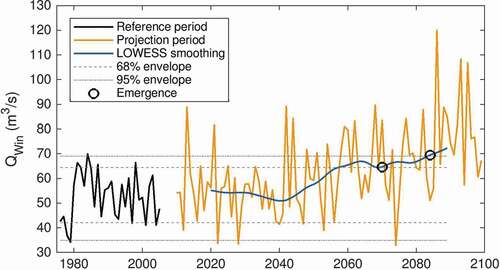
The ToE is the point in time when a climate change signal becomes distinguishable from the combined internal and inter-model variability of climate change projections, and remains so for the foreseeable future (Giorgi and Bi 2009). Internal variability is the natural inter-annual or interdecadal variability, at least as captured by the models. Inter-model variability reflects uncertainty in the process representations among the different models. How the signal is defined and how the internal and inter-model variability are accounted for varies from study to study. In this study, the climate change signal for each river location and individual GCM-RCP combination is encapsulated by the annual series of the six hydrological metrics after Locally Weighted Scatterplot Smoothing (LOWESS) smoothing using a 20-year window (Hawkins et al. 2020). Smoothing seeks to remove short-term hydro-climatic fluctuations, leaving any underlying long-term pattern. The first and last 10 years of the smoothed series are discarded from the analysis as they reflect less than 20 years’ worth of simulation data.

Internal variability for each simulation (GCM-RCP combination) is quantified at two levels of significance by taking the upper and lower thresholds bounding the central 68% and 95% of the reference period annual series (i.e. 34% and 47.5% of the data points on either side of the median), again at each river location. These levels are chosen to correspond to one and two standard deviations, as used in other ToE studies (e.g. Frame et al. 2017), although the hydrological data not are necessarily normally distributed.

Emergence for an individual location and simulation is defined here to occur when the LOWESS smoothed annual series departs the bounds of internal variability, either the upper or lower, and remains outside the bounds until the end of the smoothed simulation data – 2089. This is illustrated in Fig. 1. Emergence for the GCM-ensemble of simulations is taken to occur when a sufficient number of individual GCMs agree on emergence, akin to Mahlstein et al. (2012). For the sake of sensitivity analysis, agreement among three, four and five of the six GCMs is considered, representing increasingly stringent emergence criteria, which addresses variability among models. Accounting for inter-model variability in this way achieves an important degree of robustness in the results considering climatic response uncertainty. A larger suite of GCMs is often used in ToE analysis; however, at this time hydrological simulations across New Zealand under climate change projections are only available for six (Collins 2020).

Figure 1. Analytical derivation of the time of emergence. Annual series during the reference period (black) define the 68% and 95% internal uncertainty envelopes (grey) which set the bars beyond which the LOWESS smoothed series (blue), derived from the annual projection period series (orange), must cross and remain crossed for emergence (circles)

Results

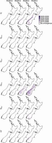
ToE varies with the hydrological metric, river reach and RCP. Considering, first, the less stringent emergence criteria of 68% reference period variability and at least three agreeing GCMs, most emergence is seen in $\bar{Q}$_Win, followed by $\bar{Q}$, and then AF and $\bar{Q}$_Sum (Fig. 2). Regions with the most emergent climate change signals are the west of the South Island, expanding to include inland and southern parts of the island. There are areas on the east of both islands that also exhibit emergence, but they are scarce. Emergence becomes earlier and more extensive under increasingly higher emissions scenarios, with a climate change signal becoming detectable under the above criteria across most of the South Island under RCP8.5, while very few river locations exhibit emergence under RCP2.6.

Figure 2. Times of emergence for six hydrological metrics across four RCPs using the emergence criteria of 68% reference period variability and three agreeing GCMs

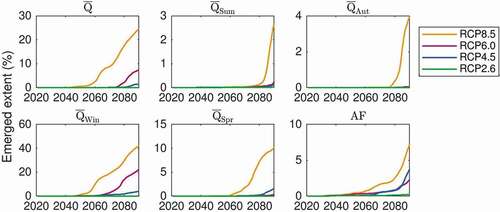
Looking at the national areal extent of emergence as a function of time, again for the less stringent criteria considered previously, offers another way to view the effects of hydrological metric, location and RCP (Fig. 3). Emerged extent rises further under RCP8.5 for all metrics than for other RCPs: 42% for $\bar{Q}$_Win under RCP8.5. Very little emergence occurs by mid-century for any metric, and in some instances no substantial emergence occurs during the entire simulation period. However, while the emerged extent generally rises earlier and further for higher RCPs, $\bar{Q}$_Spr and the annual flood present departures from this generalization, with RCP4.5 climbing further than RCP6.0. Inspecting the emerged extents under more stringent emergence criteria (not shown), these departures disappear, suggesting that they are artefacts of a limited number of realizations that can allow climate variability to be falsely identified as climate change.

Figure 3. National emerged extents for six hydrological metrics over the course of the century under each RCP. For emergence, three GCMs must agree in relation to the 68% envelope of reference period data

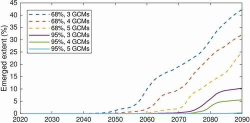
The timing and extent of emergence also depend on the stringency of the emergence criteria, as seen for $\bar{Q}$_Win under RCP8.5 (Fig. 4). Differences in emerged extent are greater when comparing the two thresholds of reference period uncertainty (68% of the annual data or 95%) than with the minimum number of agreeing GCMs required for emergence (three, four, or five of the six). Emerged extent by 2089 climbs to 42% under the combination of 68% and three GCMs, as stated previously, but only to 0.4% under 95% and five GCMs. This highlights the sensitivity of the results to the statistical and robustness criteria of the emergence test.

Figure 4. National emerged extents for $\bar{Q}$_Win under RCP8.5 for different reference period variability envelopes (68% and 95%) and the minimum number of agreeing GCMs (3, 4, or 5)

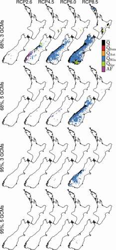
Examining the ToE among hydrological metrics together now allows us to identify which is more likely to emerge first. This offers us a way to sidestep the high uncertainties of the ToEs themselves while still providing potentially useful information for management purposes. Figure 5 shows the first emerging metric across the country, RCPs, and four emergence criteria. Again, little emergence is detected under RCP2.6, irrespective of emergence criteria, and the more stringent the criteria the less the emergence. The hydrological metric that emerges first most extensively across the RCPs and criteria is $\bar{Q}$_Win, predominantly along the west of the South Island, as well as, for the higher emissions scenarios, inland and southern South Island and eastward-flowing alpine-fed rivers. $\bar{Q}$ is the metric with the next most extensive coverage, lying mostly along the west coast of the South Island. The emergence of climate change signals in the major eastward-flowing rivers of the South Island reflects their high-precipitation source areas in the mountains, which provides a contrast with sub-alpine and lowland rivers on the east of the island which are less sensitive to prevailing climatic change.

Figure 5. First hydrological metrics to emerge under different emergence criteria (68% or 95% variability bounds, and the minimum number of agreeing GCMs) and RCPs

Bearing in mind that winter flows tend to contribute the most to annual flows, the emergence of $\bar{Q}$ before $\bar{Q}$_Win in places suggests that winter flows cannot be the sole driver of emergence at the annual scale. Referring to Fig. 2, we can see that spring and autumn flows likely play a supporting role along the very west of the South Island, and summer flows to a lesser degree along the mountain range. This latter point may stem from earlier melting of snow and ice after winter has less of an effect on flows than changes in precipitation.

Figure 5 also contains small pockets of first emergence by $\bar{Q}$_Spr and AF under the less stringent criteria, but these pockets disappear when agreement across five GCMs is required for emergence. These pockets, as mentioned above, are most likely artefacts of climate variability falsely identified as change due to the limited number of realizations.

Discussion

Times and extents of climate change emergence have been estimated for six hydrological metrics across New Zealand’s rivers subject to four climate change scenarios over the 21^st century. Emergence is more extensive and earlier under the higher-end warming scenarios, but in all cases is projected to occur only in a minority of river reaches by the end of the century. The first hydrological metric to exhibit emergence varies with location and RCP, but is most often the mean winter flow, followed by the mean flow and the annual flood. And when emergence does occur, it does so more in the country’s South Island and along the west coast.

Comparisons with other hydrological ToE studies are constrained by the limited number of such studies and differences in definitions and methods. In examining ToE of winter and summer flows across the coterminous US, Leng et al. (2016) showed emergence mostly occurring in the second half of the century, varying across the study region, increasing with greater warming, and emerging earlier and more extensively for winter flow. For a single Chinese catchment under the high-end RCP8.5 scenario, Zhuan et al. (2018) noted that dry season flows exhibited emergence earlier than wet season and annual flows under a more permissive emergence criterion, but later under a less permissive one, and again mostly after mid-century. Examining the emergence of climate change signals in two alpine catchments in France, Vidal et al. (2016) reported that winter low flow trends emerged in one catchment but not the other, while emergence in summer low flows for the two catchments occurred within a few years of one another. Lastly, under the A1B Special Report on Emissions Scenarios (SRES) scenario, Koplin et al. (2014) reported emergence in mean monthly flows varying across Switzerland from near future to late century to not at all; however, their definition of ToE did not require a statistically significant departure from reference conditions to be sustained until the end of the century; they compared reference conditions to one of two 20-year periods in the future.

The choice of statistical test is thus an important one. Like Koplin et al. (2014), Collins (2020) compared reference conditions to two future periods using a significance test (t-test applied to pooled multimodel and multiyear data) without the requirement for sustained emergence, but – of particular relevance to the present study – they used the same model simulations across New Zealand as are used here. The key difference in results is that significant climate change effects are identified more extensively using the method of Collins (2020) than in the current study. This may be because of the requirement for sustainable emergence or because of differences in detectability thresholds. In any case, this serves as a warning that quantitative projections of ToE are sensitive to the choice of statistical test, and adaptation planning may need to consider ToE estimates in more qualitative or relative terms.

Whether a climate change signal emerges locally or not depends on the magnitude of the signal in relation to the natural hydrological variability and inter-model variability. The low detection rates across New Zealand thus reflect extensive areas of low signal-to-noise ratios. New Zealand is notable for its high climatic variability that varies across the country and seasons (Salinger et al. 2004); however, no ToE study has yet been performed for New Zealand’s climate variables. Compounding the challenge of detection, emergence in river flows may lag those in both temperature and precipitation (Zhuan et al. 2018).

The timing, extent and, to a lesser degree, order of emergence also depends on the choice of criteria used to detect emergence. As emergence requires a climate change signal to become larger than a threshold of natural variability, the lower the threshold, the more permissive the test and the more emergence is identified. Similarly, as emergence requires agreement of a sufficient signal-to-noise ratio across models, then the fewer the models required for agreement, the more permissive the test and again the more emergence is identified. In other words, less stringent criteria can allow climate variability to be falsely identified as climate change, particularly given the limited number of ensembles used here. This sensitivity is to be expected and is reported elsewhere (Koplin et al. 2014, Zhuan et al. 2018), but it also highlights the subjectivity of the results. Taken to an extreme, the most stringent of criteria considered here – an internal variability threshold of 95% of reference period annual values and a minimum of five agreeing GCMs – produces negligible emergence for all hydrological metrics considered under all RCPs, and consequently no actionable information for management purposes. There is thus a balance to be struck between the detection of false positives (variability masquerading as change) and sufficient true positives to inform decision making.

The earlier and more extensive emergence of mean winter flows in the South Island can be interpreted in terms of regional hydrological variability and the nature of climate change to be experienced by New Zealand. Located in the southwest Pacific, New Zealand is projected to experience an increase in westerly airflow under climate change, particularly during winter (Ministry for the Environment 2018). This would bring more moisture to the country’s west, and because of the orographic effects of the South Island’s Southern Alp this additional precipitation would fall primarily along the west and alpine areas of the South Island. Additionally, higher air temperatures would have a disproportionate effect on river flow in snow-affected alpine areas, shifting runoff from spring to winter (Gobiet et al. 2014, Lobanova et al. 2018). Winter is also the season when precipitation and river flows for the west and alpine areas of the South Island are generally lower (Duncan and Woods 2004). The coincidence of lower winter flows and a higher winter trend thus translates to earlier and more robust emergence.

An important limitation of this study, however, is the range of models used to encapsulate inter-model variability. For the driving GCMs, six well-validated models are used to project regional sea surface temperature boundary conditions (Ministry for the Environment 2018). Most other ToE studies use more (Mahlstein et al. 2012, King et al. 2015). Moreover, the downscaling, bias-correction and hydrological modelling relied upon here are implemented using just a single model each (Collins 2020). This eliminates any consideration of uncertainty and inter-model variability over these model steps. So, while an ensemble of models would produce a more robust picture of the magnitudes of hydrological change (Hakala et al. 2020), estimates of times and extents of emergence would also change. It would thus be advisable to extend this research to include a suite of models at every stage of the climate-model cascade.

Also not considered in this study, but not irrelevant, is the period over which the analyses were conducted: 20 years. As with the RCPs and emergence criteria, this could also have been explored with a sensitivity analysis. Too short, and the inter-annual statistics would have had little time to converge; too long, and they would obscure the creeping effects of climate change. Twenty years was chosen as a nominal middle ground.

Using these results and limitations to inform mitigation and adaptation, there are several implications to note. Firstly, the results along the RCP gradient echo the common conclusion that reductions in global greenhouse gas emissions would reduce the adverse hydrological effects of climate change (IPCC 2014), and reduce the amount of adaptation needed. Secondly, hydrological processes and metrics in some regions are more sensitive to climate change than others (Lobanova et al. 2018, Byun et al. 2019). Not only may they be used as sentinels of hydrological change elsewhere in New Zealand, but they may also help focus the earlier adaptation interventions. Thirdly, the earlier emergence of changes in mean winter flows, in particular, make the metric a viable hydrological sentinel. This emphasizes the importance of hydrological monitoring (Kundzewicz et al. 2008), and in particular maintaining quality-controlled flow measurements during winter and improving our understanding of wintertime variability. Lastly, uncertainties in and the statistical nature of the estimates of the ToE mean that climate change detection will lag effects. Adaptation would then need to be pre-emptive, and potentially based on less stringent statistical tests. Waiting until climate change effects can be detected in river flow records statistically would mean missing the opportunity to adapt in a timelier manner.

Conclusions

This paper presents a method for estimating the national times of emergence for a suite of river hydrological metrics under climate change for New Zealand, and the subsequent identification of the metrics to emerge first. Changes in mean winter flows tend to emerge earlier and more extensively than other metrics, making the metric a viable hydrological sentinel. This is linked to higher temperatures and the increased westerly airflow across the country bringing more precipitation in winter to the west of the South Island. Changes in mean annual flows also exhibit appreciable emergence, stemming largely from changes in winter flows, and as such tend to lag behind winter emergence. Emergence is generally located within the South Island, and within that more so along the west and south of the island. Little emergence is projected before the middle of century or under the lower global warming scenarios, and many rivers show no emergence at all.

A significant factor controlling the timing and extent of emergence is the stringency of the emergence test itself. Using the 68% envelope of reference period data as a bound for detectability leads to substantially more emergence than the 95% envelope. Similarly, a minimum of three agreeing GCMs leads to more emergence than the minimum of four, and more again than with a minimum of five agreeing GCMs. These results illustrate the dependence and uncertainty of estimates of times and extents of emergence on choices in statistical analysis. While the emergence no earlier than mid-century may be robust, timing thereafter is not. This severely constrains the usefulness of times of emergence in quantitative water resource management applications. However, by considering the order of emergence across the metrics instead of their times, the earliest emergence of changes in mean winter flows does stand out as a robust finding, which may inform active monitoring programmes within adaptive management plans.

Acknowledgements

I am grateful for the financial support from the Deep South National Science Challenge under MBIE contract C01X1412 to conduct the analysis. Thanks also to Christian Zammit for the original hydrological simulations, carried out under Climate Changes, Impacts and Implication (MBIE contract C01X1225), and to Jim Griffiths and two anonymous reviewers for helpful feedback on the manuscript.

Disclosure statement

No potential conflict of interest was reported by the author.

Additional information

Funding

This work was supported by the Deep South National Science Challenge [C01X1412].

References

- Anagnostopoulou, C., et al., 2008. Performance of the general circulation HadAM3P model in simulating circulation types over the Mediterranean region. International Journal of Climatology, 28 (2), 185–203. doi:https://doi.org/10.1002/joc.1521
- Arnell, N.W. and Gosling, S.N., 2013. The impacts of climate change on river flow regimes at the global scale. Journal of Hydrology, 486, 351–364. doi:https://doi.org/10.1016/j.jhydrol.2013.02.010
- Bloschl, G., et al., 2017. Changing climate shifts timing of European floods. Science, 357 (6351), 588–590. doi:https://doi.org/10.1126/science.aan2506
- Booker, D.J. and Woods, R.A., 2014. Comparing and combining physically-based and empirically-based approaches for estimating the hydrology of ungauged catchments. Journal of Hydrology, 508, 227–239. doi:https://doi.org/10.1016/j.jhydrol.2013.11.007
- Bormann, H. and Pinter, N., 2017. Trends in low flows of German rivers since 1950: comparability of different low-flow indicators and their spatial patterns. River Research and Applications, 33 (7), 1191–1204. doi:https://doi.org/10.1002/rra.3152
- Byun, K., Chiu, C.M., and Hamlet, A.F., 2019. Effects of 21st century climate change on seasonal flow regimes and hydrologic extremes over the Midwest and Great Lakes region of the US. Science of the Total Environment, 650, 1261–1277. doi:https://doi.org/10.1016/j.scitotenv.2018.09.063
- Caloiero, T., 2015. Analysis of rainfall trend in New Zealand. Environmental Earth Sciences, 73 (10), 6297–6310. doi:https://doi.org/10.1007/s12665-014-3852-y
- Carey-Smith, T., Henderson, R., and Singh, S., 2018. High intensity rainfall design system version 4. Wellington, New Zealand: NIWA, 73.
- Clark, M.P., et al., 2008. Hydrological data assimilation with the ensemble Kalman filter: use of streamflow observations to update states in a distributed hydrological model. Advances in Water Resources, 31 (10), 1309–1324. doi:https://doi.org/10.1016/j.advwatres.2008.06.005
- Collins, D.B.G., 2020. New Zealand river hydrology under late 21st century climate change. Water, 12 (8), 2175. doi:https://doi.org/10.3390/w12082175
- Diffenbaugh, N.S. and Scherer, M., 2011. Observational and model evidence of global emergence of permanent, unprecedented heat in the 20th and 21st centuries. Climatic Change, 107 (3–4), 615–624. doi:https://doi.org/10.1007/s10584-011-0112-y
- Do, H.X., Westra, S., and Leonard, M., 2017. A global-scale investigation of trends in annual maximum streamflow. Journal of Hydrology, 552, 28–43. doi:https://doi.org/10.1016/j.jhydrol.2017.06.015
- Doll, P., et al., 2015. Integrating risks of climate change into water management. Hydrological Sciences Journal-Journal Des Sciences Hydrologiques, 60 (1), 4–13. doi:https://doi.org/10.1080/02626667.2014.967250
- Duncan, M. and Woods, R., 2004. Flow regimes. In: J. Harding, et al., eds. Freshwaters of New Zealand. Christchurch, New Zealand: New Zealand Hydrological Society and New Zealand Limnological Society, 7.1–7.14.
- Frame, D., et al., 2017. Population-based emergence of unfamiliar climates. Nature Climate Change, 7 (6), 407-+. doi:https://doi.org/10.1038/nclimate3297
- Giorgi, F. and Bi, X.Q., 2009. Time of emergence (TOE) of GHG-forced precipitation change hot-spots. Geophysical Research Letters, 36 (6), L06709. doi:https://doi.org/10.1029/2009GL037593
- Gobiet, A., et al., 2014. 21st century climate change in the European Alps-A review. Science of the Total Environment, 493, 1138–1151. doi:https://doi.org/10.1016/j.scitotenv.2013.07.050
- Gudmundsson, L., et al., 2019. Observed trends in global indicators of mean and extreme streamflow. Geophysical Research Letters, 46 (2), 756–766. doi:https://doi.org/10.1029/2018GL079725
- Haasnoot, M., et al., 2013. Dynamic adaptive policy pathways: a method for crafting robust decisions for a deeply uncertain world. Global Environmental Change-Human and Policy Dimensions, 23 (2), 485–498. doi:https://doi.org/10.1016/j.gloenvcha.2012.12.006
- Hakala, K., et al., 2020. Hydrological modelling of climate change impacts. In: P. Maurice, eds. Encyclopedia of water: science, technology, and society. Hoboken, USA: WIley, 1–20.
- Hanak, E. and Lund, J.R., 2012. Adapting California’s water management to climate change. Climatic Change, 111 (1), 17–44. doi:https://doi.org/10.1007/s10584-011-0241-3
- Harrington, L., et al., 2014. The role of anthropogenic climate change in the 2013 drought over North Island, New Zealand. Bulletin of the American Meteorological Society, 95 (9), S45–S48.
- Harrington, L.J., et al., 2016. Poorest countries experience earlier anthropogenic emergence of daily temperature extremes. Environmental Research Letters, 11 (5), 055007. doi:https://doi.org/10.1088/1748-9326/11/5/055007
- Hawkins, E., et al., 2020. Observed emergence of the climate change signal: from the familiar to the unknown. Geophysical Research Letters, 47 (6). doi:https://doi.org/10.1029/2019GL086259
- Hay, L.E., Markstrom, S.L., and Ward-Garrison, C., 2011. Watershed-scale response to climate change through the Twenty-First Century for selected basins across the United States. Earth Interactions, 15 (17), 1–37. doi:https://doi.org/10.1175/2010EI370.1
- IPCC, 2013. Climate Change 2013: the physical science basis. Contribution of working group I to the fifth assessment report of the intergovernmental panel on climate change. Cambridge, UK: Cambridge University Press.
- IPCC, 2014. Climate change 2014: impacts, adaptation, and vulnerability. Part A: global and sectoral aspects. Contribution of working group II to the fifth assessment report of the intergovernmental panel on climate change. Cambridge, UK: Cambridge University Press.
- Jones, P.D., et al., 2012. Hemispheric and large-scale land-surface air temperature variations: an extensive revision and an update to 2010. Journal of Geophysical Research: Atmospheres, 117 (D5), D05127. doi:https://doi.org/10.1029/2011JD017139
- Keller, K.M., Joos, F., and Raible, C.C., 2014. Time of emergence of trends in ocean biogeochemistry. Biogeosciences, 11 (13), 3647–3659. doi:https://doi.org/10.5194/bg-11-3647-2014
- King, A.D., et al., 2015. The timing of anthropogenic emergence in simulated climate extremes. Environmental Research Letters, 10 (9), 094015. doi:https://doi.org/10.1088/1748-9326/10/9/094015
- Koplin, N., et al., 2014. Robust estimates of climate-induced hydrological change in a temperate mountainous region. Climatic Change, 122 (1–2), 171–184. doi:https://doi.org/10.1007/s10584-013-1015-x
- Kundzewicz, Z.W., et al., 2008. The implications of projected climate change for freshwater resources and their management. Hydrological Sciences Journal-Journal Des Sciences Hydrologiques, 53 (1), 3–10. doi:https://doi.org/10.1623/hysj.53.1.3
- Lawrence, J., et al., 2013. Exploring climate change uncertainties to support adaptive management of changing flood-risk. Environmental Science & Policy, 33, 133–142. doi:https://doi.org/10.1016/j.envsci.2013.05.008
- Leng, G.Y., et al., 2016. Emergence of new hydrologic regimes of surface water resources in the conterminous United States under future warming. Environmental Research Letters, 11 (11), 114003. doi:https://doi.org/10.1088/1748-9326/11/11/114003
- Lobanova, A., et al., 2018. Hydrological impacts of moderate and high-end climate change across European river basins. Journal of Hydrology-Regional Studies, 18, 15–30. doi:https://doi.org/10.1016/j.ejrh.2018.05.003
- Lyu, K.W., et al., 2014. Time of emergence for regional sea-level change. Nature Climate Change, 4 (11), 1006–1010. doi:https://doi.org/10.1038/nclimate2397
- Mahlstein, I., et al., 2012. Perceptible changes in regional precipitation in a future climate. Geophysical Research Letters, 39 (5), L05701. doi:https://doi.org/10.1029/2011GL050738
- Maraun, D., 2013. When will trends in European mean and heavy daily precipitation emerge? Environmental Research Letters, 8 (1), 014004. doi:https://doi.org/10.1088/1748-9326/8/1/014004
- McMillan, H.K., Booker, D.J., and Cattoen, C., 2016. Validation of a national hydrological model. Journal of Hydrology, 541, 800–815. doi:https://doi.org/10.1016/j.jhydrol.2016.07.043
- Meyer, E.S., Characklis, G.W., and Brown, C., 2017. Evaluating financial risk management strategies under climate change for hydropower producers on the Great Lakes. Water Resources Research, 53 (3), 2114–2132. doi:https://doi.org/10.1002/2016WR019889
- Milly, P.C.D., et al., 2008. Climate change - stationarity is dead: whither water management? Science, 319 (5863), 573–574. doi:https://doi.org/10.1126/science.1151915
- Ministry for the Environment, 2018. Climate change predictions for New Zealand: atmospheric projections based on simulations undertaken for the IPCC 5th assessment. 2nd ed. Wellington, New Zealand: Ministry for the Environment, 131.
- Ministry for the Environment, 2020. National policy statement for freshwater management 2020. Wellington, New Zealand: Ministry for the Environment.
- Mullan, A.B., et al., 2010. Report on the review of NIWA’s ‘seven-station’ temperature series. Wellington, New Zealand: NIWA, 175.
- Pechlivanidis, I.G., et al., 2017. Analysis of hydrological extremes at different hydro-climatic regimes under present and future conditions. Climatic Change, 141 (3), 467–481. doi:https://doi.org/10.1007/s10584-016-1723-0
- Pohl, E., et al., 2020. Emerging climate signals in the Lena River catchment: a non-parametric statistical approach. Hydrology and Earth System Sciences, 24 (5), 2817–2839. doi:https://doi.org/10.5194/hess-24-2817-2020
- Rosier, S., et al., 2015. Extreme rainfall in early July 2014 in Northland, New Zealand-was there an anthropogenic influence? Bulletin of the American Meteorological Society, 96 (12), S136–S140. doi:https://doi.org/10.1175/BAMS-D-15-00105.1
- Salinger, J., et al., 2004. Atmospheric circulation and precipitation. In: J. Harding, et al., eds. Freshwaters of New Zealand. Christchurch, New Zealand: New Zealand Hydrological Society and New Zealand Limnological Society, 2.1–2.18.
- Van Vuuren, D.P., et al., 2011. The representative concentration pathways: an overview. Climatic Change, 109 (1–2), 5–31. doi:https://doi.org/10.1007/s10584-011-0148-z
- Vidal, J.P., et al., 2016. Hierarchy of climate and hydrological uncertainties in transient low-flow projections. Hydrology and Earth System Sciences, 20 (9), 3651–3672. doi:https://doi.org/10.5194/hess-20-3651-2016
- Wilby, R.L., 2006. When and where might climate change be detectable in UK river flows? Geophysical Research Letters, 33 (19), L19407. doi:https://doi.org/10.1029/2006GL027552
- Williamson, C.E., et al., 2009. Lakes and reservoirs as sentinels, integrators, and regulators of climate change. Limnology and Oceanography, 54 (6), 2273–2282. doi:https://doi.org/10.4319/lo.2009.54.6_part_2.2273
- Woods, R., et al., 2006. Estimating mean flow of New Zealand rivers. Journal of Hydrology (NZ), 45 (2), 95–110.
- Zhuan, M.J., et al., 2018. Timing of human-induced climate change emergence from internal climate variability for hydrological impact studies. Hydrology Research, 49 (2), 421–437. doi:https://doi.org/10.2166/nh.2018.059