Precipitation extremes derived from temporally aggregated time series and the efficiency of their correction

ABSTRACT

Extreme precipitation intensities derived from temporally aggregated time series can be considerably underestimated. Therefore, some form of correction is appropriate prior to their usage e.g. for the derivation of idf curves. The correction is usually performed in a multiplicative manner, using the coefficient obtained as a mean ratio of real to aggregated extremes. In this paper a novel correction approach is derived, allowing an individual treatment of each aggregated extreme. The precipitation time series from Prague (central Europe) are used for the assessment of newly introduced method. The comparison with the standard approach shows that the new method reaches better results as it reduces an undesirable overestimation of the corrected extremes. Moreover, the effect of data aggregation on extreme precipitation intensities is evaluated as well as the effect on quantiles of the generalized extreme value (GEV) distribution. The results are compared to those published for other climatic conditions.

KEYWORDS:

• precipitation extremes
• rainfall data
• temporal aggregation
• underestimation
• correction
• GEV distribution

Editor A. Castellarin Associate editor S. Vorogushyn

1 Introduction

The knowledge of extreme precipitation intensities is of high importance in many research and practical areas. Specifically, for the design purposes the time series of annual maximum rainfall intensities for a various set of durations are necessary to establish the intensity-duration-frequency (idf) relationships at a given locality (Willems 2000). Such analyses are always connected with a substantial uncertainty related to limited data sources, to methods used to derive extremes from the data or to a non-stationarity in time series (Lima et al. 2018, Lee and Singh 2020).

Another source of uncertainty is represented by a time resolution of historical rainfall records, which are necessary for the analyses. Morbidelli et al. (2020, 2021) analysed a temporal resolution of precipitation time series across a large number of geographical areas and concluded, that although there are approximately 250,000 of the measurement stations worldwide, long time series with the time resolution lower than 1 hour are rarely available. In many countries the measurement in 1-minute time step started within the last decade of the 20-th century, nevertheless; in many areas (e.g. Bangladesh, north-east region of Brazil) such data are not available at all. The time resolution of rainfall data plays an important role within the analyses. While the precipitation extremes derived from data with 1-minute time step can be considered undistorted (Morbidelli et al. 2017), the extremes derived from data with a lower temporal resolution can be considerably underestimated. Therefore, if only aggregated data are available, the underestimation should be considered and some form of correction should be applied.

The underestimation comes from the fact, that the starting point of real maximum precipitation seldom coincides with the time step of measurement, a real extreme is therefore split into two (or more) time steps. The intensity of such smoothing depends on the time step of measurement ($t$) and on the rain duration ($d$), the ratio $t/d$ is usually denoted as sampling ratio ($sr$). The underestimation is usually evaluated through the mean ratio of real to aggregated extreme intensities, hereafter we denote this ratio as $\alpha$ (the terms conversion factor or sampling adjustment factor can be found in literature). The value of $\alpha$ is used to correct the aggregated extremes in a multiplicative manner. Obviously, the highest error occurs for $sr=1$ (i.e. for $t=d$) where $\alpha$ for individual extremes vary from 1 to 2; Fig. 1 schematically illustrates two examples corresponding to the possible lowest ($\alpha =1$) and the highest error ($\alpha =2$).

Figure 1. The underestimation of the precipitation intensity (or depth) in measurement with a fixed time step corresponding to a duration of the rain: (a) the perfect match when no correction is needed, the ratio $\alpha$ of the real to the aggregated intensity is 1; (b) only a half of the real precipitation is registered, which represents the maximum possible underestimation of aggregated extreme (α = 2). The latter case is conditioned by the absence of additional rain next to the location of extreme rain event

The underestimation naturally decreases when the duration of interest $d$ is higher than the time step $t$. In such case an error occurs only on boundaries of the rain (i.e. in the first and the last time steps), the inner part is registered accurately. Morbidelli et al. (2017) found that the error is negligible for $sr<0.1$.

The underestimation was described and quantified several times in the literature. Hershfield (1961) analysed the data from many stations across the USA and found a mean $\alpha$ equal to 1.13. The value of $\alpha$ was found independent on the duration since the same coefficient 1.13 was obtained for the durations 1 hour and 1 day, both for $t=d$. Weiss (1964) used a probabilistic approach and under the assumption of uniform temporal rainfall distribution derived that the mean $\alpha =8/7=1.143$ for $sr=1$. The result was obtained as an inverse of the expected portion of the rain depth registered in a fixed time interval. Young and McEnroe (2003) used the data from the Kansas City region and empirically derived the relation between $\alpha$ and the sampling ratio. For $sr=1$ their relation gives the value of $\alpha =1.13$, which is the same as the result reached by Hershfield (1961). They also concluded that there is no obvious relation between $d$ and $\alpha$. Yoo et al. (2015) analysed on a theoretical basis the effect of various temporal rainfall distributions on the value of $\alpha$. For a uniformly distributed rain they found that $\alpha =4/3=1.33$ (in contrast to the Weiss’s result 1.143), for other analysed time distributions the values of $\alpha$ were lower. Their work also summarises the empirical values of $\alpha$ used worldwide for a correction of aggregated rainfall data, ranging for daily values approximately from 1.13 (USA) to 1.17 (UK, Australia), see an introduction of Yoo et al. (2015) for details. Papalexiou et al. (2016) analysed a large number of rainfall records in 1-hour time step across the USA and proposed a slightly different formulation of the correction factor, including its statistical distribution. Morbidelli et al. (2017) used the data from Central Italy to derive 3 relations between $\alpha$ and the sampling ratio (with respect to different durations) and also analysed the length of time series necessary to an adequate assessment of the underestimation of precipitation extremes. Morbidelli et al. (2018a) analysed in detail the errors caused by data aggregation and found that for individual extremes the errors follow an exponential distribution and are inversely proportional to rainfall depths. Morbidelli et al. (2018b) found that the aggregation has a considerable effect on the trend analyses of the annual precipitation maxima. Llabres-Brustenga et al. (2020) analysed the effect of regional and seasonal rainfall patterns on the value of $\alpha$ for the time series in 1-day time step across the Catalonia.

The main aim of this paper is to present a novel approach to the correction of aggregated extremes. The novelty consists in the fact that neighbouring data surrounding each aggregated extreme provide a useful information about possible correction limits. Therefore, each aggregated extreme can be corrected individually which effectively reduces the inaccuracy introduced by the correction itself. The efficiency of the correction is analysed and compared with the standard approach. Moreover, the effect of data aggregation on extreme precipitation intensities is analysed as well as the effect on quantiles of the generalized extreme value (GEV) distribution. The data from Prague (central Europe) are used and the results are compared to those published for other climatic conditions. We note that only $sr=1$ is considered in the paper, as it brings the highest underestimation of aggregated extremes.

2 Study area and data

The precipitation data from Prague, the capital of the Czech Republic, were used in this study. According to Köppen climate classification the site lies on a boundary between Cfb and Dfb climate zones characterised by a temperate oceanic/humid continental climate with approximately uniform precipitation distribution and warm summers (Tolasz 2007). Specifically, the annual precipitation pattern can be characterized as transitional between oceanic and continental climate with prevailing summer rainfalls (Mikolášková 2009). In the 1981–2010 period the summer precipitation totals (355 mm) were on average twice as high as winter ones (165 mm), the mean annual temperature was 9.4°C and the mean annual precipitation was 520 mm.

There are 23 gauging stations in the Prague region operated by the city administrator since the year 1999. During the period of interest, the observation network was partly adjusted, therefore not all available data was finally used in the study. To preserve a homogeneity of the observations only 16 gauging stations were finally chosen for the evaluation, covering the 21-years period from 1999 to 2019; see Fig. 2 for the details of the area.

Figure 2. The location of considered gauging stations in Prague (Czech Republic)

The data in 1-minute time step were measured by the automatic tipping rain gauge (Fiedler SR03, CZE). The measurement accuracy at each station has been regularly adjusted by the static and dynamic calibration. The quality control and error checking of the rainfall database were carried out prior to the study.

3 Methods

3.1 Derivation of rainfall extremes

The extreme rainfall intensities for the durations 5 minutes, 30 minutes, 1 hour, 3 hours, 6 hours, 12 hours and 24 hours were derived from the original 1-minute data in two ways. In the first way the time series with a fixed time step corresponding to given duration was obtained by aggregating of the original data. For example, for the 5-minutes duration, the first time-step was obtained as a mean intensity from the first 5 measurements (minutes 1–5), the second analogously from the minutes 6–10 etc. The collection of 21 annual extreme intensities was obtained from the aggregated time series, hereafter we refer to these maxima as “aggregated” extremes. In the second way the floating window (overlapping moving averages) with a width corresponding to given duration was used to obtain another collection of annual maxima; we refer to these maxima as “real” extremes.

In fact, our collections of real extremes are not real indeed, as they also originate from the aggregated data (with a 1-minute time step). Nevertheless, such extremes better describe the extreme rainfalls at given location than the aggregated ones. Furthermore, Morbidelli et al. (2017) showed that the effect of 1-minute aggregation is negligible.

3.2 GEV distribution

According to the Extreme values theorem a distribution of block maxima of a time series converges to the generalized extreme value (GEV) distribution (e.g. Tabari 2021). The convergence is conditioned by the independence of individual events, which must be derived from the blocks of sufficient length and must be generated by the same underlying mechanism (Wilks 2011). The GEV distribution is frequently used for the description of rainfall extremes (e.g. Koutsoyiannis et al. 1998, Darwish et al. 2018, Libertino et al. 2018, Bonaccorso et al. 2020) and was applied in this study to model statistical properties of both aggregated and real extreme intensities.

The GEV distribution is given by the cumulative distribution function in the form

(1) $F\left(x\right)=exp\left\{-{\left(1-\frac{\kappa }{\alpha }\left(x-\xi \right)\right)}^{1/\kappa }\right\}$(1)

where $\xi$, $\alpha$ and $\kappa$ are the location, scale and shape parameters, respectively. The quantile function is given by

(2) $Q\left(p\right)=\xi +\frac{\alpha }{\kappa }\left(1-{\left(-\mathrm{l}\mathrm{n}p\right)}^{\kappa }\right)$(2)

The distribution parameters were fitted by the L-moments method (Hosking 1990). In order to verify the suitability of the GEV distribution for our data, the Lilliefors goodness-of-fit test was carried out for each fitted distribution. Since the critical values of the Lilliefors test for the GEV distribution are not commonly available, they have been obtained individually for each fitted dataset by a numerical simulation, see Wilks (2011), chapter 5.2.5 for details.

The particular quantiles of the distribution were associated with their mean return period (time of recurrence) according to

(3) $T\left(x\right)=\frac{1}{\omega \left(1-F\left(x\right)\right)}$(3)

where $\omega$ denotes the sampling frequency (=1 year⁻¹ in our case). The quantiles for the probabilities 0.5, 0.8, 0.9 and 0.95 corresponding to the recurrence times 2, 5, 10 and 20 years, respectively, were derived and analysed for each fitted distribution. Hereafter we refer to the quantiles derived from distributions of aggregated extremes as “aggregated” quantiles, and analogously we refer to the quantiles derived from distributions of real extremes as “real” quantiles. For the clarity of the text, the return periods are used to refer to the corresponding quantiles (e.g. the quantile for the probability 0.95 is referred as 20-years quantile etc.).

3.3 Significance of differences

A statistical significance of differences between aggregated and real quantiles was investigated. Following the bootstrap approach (Davison and Hinkley 1997) a difference between particular quantiles derived from sets of aggregated and real extremes was assessed as follows:

1. The samples of 21 annual extremes were randomly selected with replacement from both sets of original aggregated and real extremes. The parameters of GEV distribution were estimated from both samples and the quantiles were derived from both distributions. The aggregated quantile was subtracted from the real quantile and the difference was stored.

2. Step 1 was repeated 10 000 times.

3. Finally, the aggregated and real quantiles were found significantly different if the 95% confidence interval of these 10 000 sample differences did not contain zero.

Similar approach was used e.g. by Overeem et al. (2008) to assess the uncertainty connected with the derivation of idf curves.

3.4 Correction of aggregated extremes

A correction of aggregated extremes was performed in two ways. Firstly, the classical multiplicative approach was used according to

(4) $x_{\mathrm{c}}=\alpha \cdot x_{\mathrm{a}}$(4)

where the subscripts $\mathrm{c}$ and $\mathrm{a}$ denote the corrected and aggregated extremes, respectively, and the symbol $\alpha$ denotes the correction factor, derived as a mean ratio of real to aggregated extremes.

Secondly, a novel correction approach was derived. It is based on the fact, that each aggregated extreme can be corrected individually (into some extent), since we can utilize an information from its neighbouring aggregated values. Figure 1(b) shows, that in an extreme case only a half of precipitation depth is registered at given time step. In such case a real intensity can be derived as a sum of two consecutive rain depths divided by one duration. Let ${\sigma }_i$ is a highest aggregated precipitation depth, which was registered at i-th time step in a given year. Then

(5) $m=\left[\mathrm{m}\mathrm{a}\mathrm{x}\left({\sigma }_i+{\sigma }_{i-1},{\sigma }_i+{\sigma }_{i+1}\right)\right]/d$(5)

is a maximum possible real intensity associated with the measured aggregated intensity $x_{\mathrm{a}}={\sigma }_i/d$. There are two possible ways how such maxima can be considered. Firstly, we can find a highest $m$ in a given year, which represents the overall highest possible intensity (such “global” $m$ is always $\ge$ a real maximum of the year). Secondly, we can find the highest aggregated value $x_{\mathrm{a}}$ and calculate the $m$ associated with this value (such “local” $m$ can be hypothetically lower than a real maximum of the year). The latter case was adopted in our approach, since a further analysis showed that in 87% of cases there is a temporal concurrence of real and aggregated extremes in a given year (calculated for all aggregations as a whole). Such concurrences were assessed from our “neighbourhood” perspective – the real and aggregated extremes were found concurrent if a lag between their start points was $\le d$. It means, that if an aggregated extreme is analysed together with its neighbourhood (±1 duration), there is a high probability that an unknown real extreme is located somewhere inside of this interval. The values of “local” $m$ are therefore tightly connected with the real extremes and were used in our correction scheme.

If we assume that a real extreme $x_{\mathrm{r}}$ lies within the neighbourhood of an aggregated extreme $x_{\mathrm{a}}$, the values of $x_{\mathrm{a}}$ and its associated $m$ represent the lower and upper boundaries, respectively, in which the value of $x_{\mathrm{r}}$ can be searched. In other words, the corrected value $x_{\mathrm{c}}$ should not exceed the value of $m$. In a special case both neighbours of $x_{\mathrm{a}}$ are equal to 0, therefore $x_{\mathrm{a}}=m=x_{\mathrm{r}}$ and no correction is needed (this can be found approximately in 11% of cases, for all aggregations as a whole). In general, a lot of extremes are protected from an undesirable overestimation when the correction is limited from above by the value of $m$.

It was also found, that there is a strong linear relationship between the real extremes and the values of $m$ (see an analysis later). Therefore, the variable $m$ was added into the correction scheme and the multiple linear regression was applied to find the coefficients. The overall correction scheme is given by the formula

(6) $x_{\mathrm{c}}=\mathrm{m}\mathrm{i}\mathrm{n}\left(m,{\beta }_0+{\beta }_1{x}_{\mathrm{a}}+{\beta }_{2}m\right)$(6)

If the value calculated by the linear model ${\beta }_0+{\beta }_1{x}_{\mathrm{a}}+{\beta }_{2}m$ exceeds the value of m, it is reduced to m. The corrected value is therefore locally adjusted with respect to the neighbourhood of a particular aggregated extreme. Hereafter we denote this approach as the combined method, contrary to the multiplicative method given by formula (4).

To compare the efficiency of both correction methods, the stations were split into the calibration (1–8) and the validation (9–16) stations. The coefficients of both correction methods were derived from the calibration data and subsequently applied to the validation data, the comparison is presented in the Results section. Table 1 presents the coefficients including the statistical significance of the coefficients for the combined method, which were derived through the linear regression.

Table 1. The coefficients for both correction methods derived from the calibration data

method	coefficient	value	p-value
multiplicative	$\alpha$	1.146	-
combined	${\beta }_0$	0.005	0.301
	${\beta }_1$	0.81	<2e-16
	${\beta }_2$	0.22	<2e-16

The Table 1 shows that the absolute term in the formula (6) was found statistically insignificant and it was excluded from the procedure. Therefore, the combined correction was performed according to

(7) $x_{\mathrm{c}}=\mathrm{m}\mathrm{i}\mathrm{n}\left(m,0.81x_{\mathrm{a}}+0.22m\right)$(7)

The exclusion of the absolute term corresponds to the nature of problem, because when (hypothetically) $x_{\mathrm{a}}=m=0$, the linear equation $x_{\mathrm{c}}={\beta }_1{x}_{\mathrm{a}}+{\beta }_{2}m$ leads to $x_{\mathrm{c}}=0$. Figure 3 presents the relations between the variables incorporated into the combined correction method.

Figure 3. The relations between the variables incorporated into the combined correction scheme. We note that only the data from the calibration stations (for all durations) are presented here. The lines represent the identity relation

From Fig. 3(c) it is clear that there is a tight linear relation between the aggregated extremes and the values of $m$. To verify a benefit of $m$ in the correction scheme, the partial correlation coefficient between $x_{\mathrm{r}}$ and $m$ was calculated, excluding the effect of $x_{\mathrm{a}}$ from both variables. The partial correlation was 0.32 (p-value 2.2e-16, 95% confidence interval from 0.27 to 0.37), which confirmed $m$ as a valid predictor of $x_{\mathrm{r}}$.

Finally let us remark, that we tried to make the corrections more accurate by finding a specific set of coefficients for each duration. Nevertheless, no obvious pattern across the durations was found for the coefficients of both correction methods. The specific sets of coefficients only increased the complexity and had a minor effect on the results. Therefore, the formulas (4) and (6) were applied with the same coefficients across all durations.

4 Results and discussion

4.1 Real and aggregated extreme intensities

Figure 4(a) and (b) depict in detail the relations of real and aggregated extremes for shortest (5-minutes) and longest (24 hours) durations, respectively; similar plots were obtained for all remaining durations.

Figure 4. Relation of the real and the aggregated extreme intensities for (a) 5 minutes duration; (b) 24 hours duration and (c) the summary of ratios of real to aggregated intensities for all durations. The lines in figures (a) and (b) represent the identity relation

Figure 4(c) summarizes the ratios of real to aggregated extremes for all durations. The overall mean ratio of the real to the aggregated extremes was 1.146 in our data. This result is very similar to those published e.g. by Hershfield (1961), Young and McEnroe (2003) or Morbidelli et al. (2017). This indicates that the data aggregation affects extreme intensities on average in a similar way across a wide spectrum of climatic conditions and various durations. The highest ratios in our data reached 1.91. The mean ratios for particular durations fluctuated from 1.119 to 1.193., and there was no obvious pattern across the durations, similarly as in Young and McEnroe (2003).

4.2 Real and aggregated GEV quantiles

The Lilliefors goodness-of-fit test was carried out for each fitted distribution prior to the analyses of quantiles. Only in 3 cases (2 ×30 minutes duration, 1 ×6 hours duration) the GEV distribution was found unsuitable, which was approximately 1.3% from 224 tested datasets. This proved that the GEV distribution fits the block maxima well, which is in agreement with the Extreme value theory. All unsuitable distributions were excluded from the analyses.

In the majority of cases the bootstrap tests showed that the differences between the real and the aggregated quantiles are not statistically significant, which can be important for various statistical considerations. In particular, in 12 cases the difference was found significant, representing approximately 2.7% from all tested quantiles, 9 of these significant differences were found for 24 hours aggregation. Figure 5 demonstrates that the effect of temporal aggregation on the GEV quantiles is in general lower than in the case of extreme intensities (compare with Fig. 4).

Figure 5. Relation of the real and the aggregated GEV quantiles over all durations for (a) 2-years quantile; (b) 20-years quantile and (c) the summary of ratios of real to aggregated quantiles. The lines in figures (a) and (b) represent the identity relation

The overall mean ratio of real to aggregated quantiles was 1.115 and the maximum ratio reached 1.39; both these indicators are lower than in the case of extreme intensities. The relations of the lowest (2-years) and highest (20-years) real and aggregated quantiles are in detail presented in Fig. 5(a) and (b), Fig. 5(c) presents an overview of the ratios of real to aggregated quantiles. As seen from the Fig. 5(c), some real quantiles are lower than their aggregated counterparts. Such “inverse” relation was found 3 times in the cases of 10- and 20-years quantiles. It is given by the fact, that the conversion from extreme intensities to GEV quantiles is a highly nonlinear process, including the fitting of the GEV parameters and the calculation of quantile function according to relation (2). As a result of this process it can happen that while the main probability mass of the aggregated extremes is located more on the left, the overall shapes of the distributions can cause that some high quantiles of the aggregated extremes are located more on the right compared to the real ones. Therefore, while all aggregated extremes are naturally lower than or equal to their real counterparts, the GEV quantiles derived from these data does not need to satisfy such inequality. This phenomenon is more frequent in higher quantiles (with recurrence times >20 years), nevertheless these results are not presented here due to their high uncertainty related to relatively short datasets from which they were derived.

4.3 Effect of corrections

The effect of corrections on aggregated extreme intensities from the validation stations is presented in Fig. 6, which compares the ratios of the real to the corrected extremes for both methods.

Figure 6. The effect of corrections on extreme intensities. The box-plots summarise the ratios of the real extremes to: the aggregated extremes (in grey); to the extremes corrected by the multiplicative method (in white) and to the extremes corrected by the combined method (in red). The y = 1 line (in red) represents the ideal result of a correction

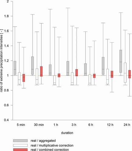
The figure clearly shows that many of extremes are overestimated (the ratio < 1) after the correction. However, the overestimation is significantly reduced in the results of the combined method. The box plots show that for the combined method the medians are in all cases closer to 1 and the inter-quartile ranges (IQR) are in all cases significantly narrower. The results of the combined method are more concentrated around the desired value 1 than in the case of the multiplicative method. On the other hand, the lower whiskers of the box-plots of the multiplicative methods are aligned on the value 0.88 across all durations, while for the combined method the whiskers are slightly farther from 1. This is given by the fact that the overestimation is limited by the ratio $1/\alpha$ in the case of multiplicative method (therefore for $x_{\mathrm{a}}=x_{\mathrm{r}}$ the corrected value is overestimated exactly 1.14-times) while the combined method has no such limitation. The situation is different for upper whiskers, which are closer to 1 for the combined method in most cases. This indicates that even the underestimation is more effectively reduced by the combined method.

The GEV quantiles were derived from the corrected data and subsequently compared with the real quantiles, the results are presented in Fig. 7.

Figure 7. The effect of corrections on GEV quantiles over all durations. The box-plots summarise the ratios of real quantiles to: the aggregated quantiles (in grey); to the quantiles derived from the extremes corrected by the multiplicative method (in white) and to the quantiles derived from the extremes corrected by the combined method (in red). The y = 1 line (in red) represents the ideal result of a correction

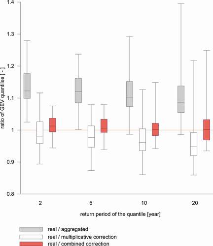
As in the case of extremes, the combined correction reduces the overestimation of corrected data. The results of the combined method are centred and more compressed around 1 (the IQRs are significantly narrower), while for the multiplicative method the results are systematically overestimated. In most cases the whiskers of box-plots (both the lower and the upper) are closer to 1 for the combined method. It is also seen from the Fig. 7 that the efficiency of corrections decreases towards high quantiles, regardless of the correction method.

Finally let us state several remarks about the applicability of the presented approach. The combined correction method is based on a logical consideration, consisting in the analysis of neighbourhoods of aggregated extremes. The idea itself is with no doubt applicable to another time series. Nevertheless, the particular coefficients were derived from our data, which are limited considerably in their temporal and spatial extent. Therefore, an application of the relation (7) to another data is connected with some uncertainty. Nevertheless, it can be seen from the literature that the coefficients for the multiplicative approach derived from time series across a wide spectrum of climatic conditions are similar, ranging approximately from 1.13 to 1.17 (Yoo et al. 2015). We have verified that an application of these adopted coefficients in formula (4) improved our raw aggregated extremes considerably, although the results were naturally worse than the results obtained with the coefficients derived from our data. It gives us a certain confidence that the relation (7) is applicable to another data without recalibration.

Another question is an applicability to coarser time resolution data (weekly, monthly etc.). The results showed that the effect of temporal aggregation and the efficiency of corrections are similar across the time scales from 5 minutes to 1 day, which encompasses the extremes originating from local convective storms as well as from stratiform rains. Nevertheless, the applicability of the proposed correction to coarser time scales should be verified prior to its usage.

Morbidelli et al. (2017) showed that the length of time series should be 15–20 years to assess the error caused by the data aggregation. From this point of view the length of our time series (21 years) is sufficient. Nevertheless, it is self-evident that the coefficients derived from longer time series would increase a plausibility of our correction formula.

5 Conclusions

In this paper the novel approach for the correction of aggregated extremes was derived. The precipitation time series from Prague (central Europe) were used for the assessment of newly introduced method. The comparison with the standard approach showed that the new method reaches better results, mainly because it effectively reduces the undesirable overestimation of the corrected extremes. Moreover, the effect of data aggregation itself was evaluated. The results showed that the underestimation of precipitation extremes was similar to the results obtained in different climatic conditions. The mean ratio of real to aggregated extreme intensities was comparable to the results published for various climatic conditions. It was also found that there is no obvious relation between the effect of aggregation and the duration of interest, which is also in agreement with the previously published results. The additional analysis showed that the effect of temporal aggregation on GEV quantiles is in general lower than the effect on precipitation extremes itself. The differences between the real and the aggregated GEV quantiles were found statistically insignificant in a majority of cases.

Acknowledgements

We thank both reviewers for their constructive comments.

Funding

This work was supported by the Czech Science Foundation [GA CR 20-00788S]; Czech Academy of Sciences [RVO 67985874].

Disclosure statement

No potential conflict of interest was reported by the author(s).

References

- Bonaccorso, B., Brigandi, G., and Aronica, G.T., 2020. Regional sub-hourly extreme rainfall estimates in Sicily under a scale invariance framework. Water Resources Management, 34 (14), 4363–4380. doi:https://doi.org/10.1007/s11269-020-02667-5
- Darwish, M.M., et al., 2018. A regional frequency analysis of UK sub-daily extreme precipitation and assessment of their seasonality. International Journal of Climatology, 38 (13), 4758–4776. doi:https://doi.org/10.1002/joc.5694
- Davison, A.C., and Hinkley, D.V., 1997. Bootstrap methods and their application. New York: Cambridge University Press.
- Hershfield, D.M., 1961. Rainfall frequency atlas of the United States for durations from 30 minutes to 24 hours and return periods from 1 to 100 years. US Weather Bureau Technical Paper N. 40, U.S. Department of Commerce, Washington, DC.
- Hosking, J.R.M., 1990. L-moments: analysis and estimation of distributions using linear combinations of order statistics. Journal of the Royal Statistical Society B, 52 (1), 105–124.
- Koutsoyiannis, D., Kozonis, D., and Manetas, A., 1998. A mathematical framework for studying rainfall intensity-duration-frequency relationships. Journal of Hydrology, 206 (1–2), 118–135. doi:https://doi.org/10.1016/S0022-1694(98)00097-3
- Lee, K. and Singh, V.P., 2020. Analysis of uncertainty and non-stationarity in probable maximum precipitation in Brazos River basin. Journal of Hydrology, 590, 125526. doi:https://doi.org/10.1016/j.jhydrol.2020.125526
- Libertino, A., et al., 2018. Regional-scale analysis of extreme precipitation from short and fragmented records. Advances in Water Resources, 112, 147–159. doi:https://doi.org/10.1016/j.advwatres.2017.12.015
- Lima, C.H.R., Kwon, H.H., and Kim, Y.T., 2018. A local-regional scaling-invariant Bayesian GEV model for estimating rainfall IDF curves in a future climate. Journal of Hydrology, 566, 73–88. doi:https://doi.org/10.1016/j.jhydrol.2018.08.075
- Llabres-Brustenga, A., et al., 2020. Influence of regional and seasonal rainfall patterns on the ratio between fixed and unrestricted measured intervals of rainfall amounts. Theoretical and Applied Climatology, 140 (1–2), 389–399. doi:https://doi.org/10.1007/s00704-020-03091-w
- Mikolášková, K., 2009. Continental and oceanic precipitation regime in Europe. Central European Journal of Geosciences, 1 (2), 176–182. doi:https://doi.org/10.2478/v10085-009-0013-8
- Morbidelli, R., et al., 2017. Effect of temporal aggregation on the estimate of annual maximum rainfall depths for the design of hydraulic infrastructure systems. Journal of Hydrology, 544, 710–720. doi:https://doi.org/10.1016/j.jhydrol.2017.09.050
- Morbidelli, R., et al., 2018a. Characteristics of the underestimation error of annual maximum rainfall depth due to coarse temporal aggregation. Atmosphere, 9 (8), 303. doi:https://doi.org/10.3390/atmos9080303
- Morbidelli, R., et al., 2018b. Influence of temporal data aggregation on trend estimation for intense rainfall. Advances in Water Resources, 122, 304–316. doi:https://doi.org/10.1016/j.advwatres.2018.10.027
- Morbidelli, R., et al., 2020. The history of rainfall data time-resolution in a wide variety of geographical areas. Journal of Hydrology, 590, 125258. doi:https://doi.org/10.1016/j.jhydrol.2020.125258
- Morbidelli, R., et al., 2021. A review on rainfall data resolution and its role in the hydrological practice. Water, 13 (8), 1012. doi:https://doi.org/10.3390/w13081012
- Overeem, A., Buishand, A., and Holleman, I., 2008. Rainfall depth-duration-frequency curves and their uncertainties. Journal of Hydrology, 348 (1–2), 124–134. doi:https://doi.org/10.1016/j.jhydrol.2007.09.044
- Papalexiou, S.M., Dialynas, Y.G., and Grimaldi, S., 2016. Hershfield factor revisited: correcting annual maximum precipitation. Journal of Hydrology, 542, 884–895. doi:https://doi.org/10.1016/j.jhydrol.2016.09.058
- Tabari, H., 2021. Extreme value analysis dilemma for climate change impact assessment on global flood and extreme precipitation. Journal of Hydrology, 593, 125932. doi:https://doi.org/10.1016/j.jhydrol.2020.125932
- Tolasz, R., 2007. Climate Atlas of Czechia. Prague: Czech Hydrometeorological Institute.
- Weiss, L.L., 1964. Ratio of true to fixed-interval maximum rainfall. Journal of the Hydraulics Division, 90 (1), 77–82. doi:https://doi.org/10.1061/JYCEAJ.0001008
- Wilks, D.S., 2011. Statistical methods in the atmospheric science. Amsterdam: Academic.
- Willems, P., 2000. Compound intensity/duration/frequency-relationships of extreme precipitation for two seasons and two storm types. Journal of Hydrology, 233 (1–4), 189–205. doi:https://doi.org/10.1016/S0022-1694(00)00233-X
- Yoo, C., Jun, C., and Park, C., 2015. Effect of rainfall temporal distribution on the conversion factor to convert the fixed-interval into true-interval rainfall. Journal of Hydrologic Engineering, 20 (10), 4015018. doi:https://doi.org/10.1061/(ASCE)HE.1943-5584.0001178
- Young, C.B. and McEnroe, B.M., 2003. Sampling adjustment factors for rainfall recorded at fixed time intervals. Journal of Hydrologic Engineering, 8 (5), 294–296. doi:https://doi.org/10.1061/(ASCE)1084-0699(2003)8:5(294)