
 ?Mathematical formulae have been encoded as MathML and are displayed in this HTML version using MathJax in order to improve their display. Uncheck the box to turn MathJax off. This feature requires Javascript. Click on a formula to zoom.
ABSTRACT
The objective of this study was to evaluate the performance of the reference evapotranspiration at the hourly and daily scale, using the Moretti-Jerszurki-Silva alternative approach (MJS; EToMJS), for the Brazilian sub-tropical climate. Data from 25 automatic weather stations were used for calibration and validation analyses. In the linear correlation between EToMJS.h and EToh (ASCE-PM), at the hourly scale, it was found that: (i) values of EToh were higher than those of EToMJS.h in the daytime, while the opposite occurred at night-time; (ii) hourly EToMJS.h and EToh curves had an average two-hour delay; and (iii) the delay correction improves the correlation between EToMJS.h and EToh. Statistically, there was better efficiency between EToh and EToMJS.h in the summer for Cfa climate and in the spring for Cfb climate. The MJS showed better efficiency concerning the Hargreaves and Samani, modified parametric and Penman-Monteith temperature models, being the best alternative methodology to estimate ETo at the daily scale in the sub-tropical region of Brazil.
Editor S. Archfield Associate Editor N. Malamos
1 Introduction
Editor S. Archfield; Associate editor N. Malamos Evapotranspiration (ET) consists of water loss to the atmosphere through soil evaporation, the ground surface and plant transpiration. It is one of the main components of the hydrological cycle, being fundamental in water planning and management in drainage basins and agricultural crops. For a better understanding of trends and interactions between climatic variables in ET, the term reference evapotranspiration (ETo) was idealized, considering a hypothetical grass reference crop, with uniform and fixed cultivation height (0.12 m for grass and 0.50 m for alfalfa), fixed surface resistance of 70 s m–1 and albedo of 0.23. The reference surface resembles an extensive grassy surface, without water restriction, experiencing active growth and completely shading the ground (Allen et al. Citation1998).
ETo is a water component that is difficult to measure directly, due to the costs for equipment such as evapotranspirometers or lysimeters, as well as the requirement for qualified labour to operate and maintain the equipment. For this reason, numerous indirect ETo estimation methods have been developed based on meteorological variables, and can be found in the literature (Alves Sobrinho et al. Citation2011, Moura et al. Citation2013, Tegos et al. Citation2013, Citation2015, Citation2017, Fenner et al. Citation2019).
Among the indirect methods, the Penman model and its derivatives are widely studied due to their physical basis. In the current literature, the American Society of Civil Engineers (ASCE-PM) model, derived from the Food and Agriculture Organization (FAO) Penman-Monteith method, is considered to be the most suitable, recognized for presenting good precision and approximation with lysimeter data. However, the ASCE-PM model is complex and requires a large amount of meteorological data (air temperature, relative humidity, wind speed and solar radiation), which is not always available, or may not be available in sufficient quantities or quality for the activity to be performed (Moura et al. Citation2013, Maina et al. Citation2014, Nolz and Rodný Citation2019).
Due to the difficulty of using highly complex methods of calculation that require many input parameters, simpler alternative methods based on fewer input parameters and climatic variables have been formulated (Owusu-Sekyere et al. Citation2017). Among the models recommended in the literature, the Hargreaves and Samani (HS; Hargreaves and Samani Citation1985), Penman-Monteith temperature (PMT; Raziei and Pereira Citation2013, Paredes et al. Citation2020b) and modified parametric (PET; Tegos et al. Citation2017) models stand out due to the simplicity and precision in obtaining daily values of evapotranspiration. The PMT approach uses the Penman-Monteith equation as a base, and the input variables are estimated with equations that consider air temperature. The wind speed is considered using default or regional average values (Raziei and Pereira Citation2013, Paredes et al. Citation2020b). Tegos et al. (Citation2017) introduced an innovative approach, the PET model for estimating potential evapotranspiration. The authors observed high efficiency of the model in relation to other important models for estimating evapotranspiration in different climatic regimes worldwide.
The ASCE-PM method (ASCE-EWRI Citation2005) allows the estimation of hourly evapotranspiration (EToh), including night-time periods. The sum over a 24-h period for EToh integrates the values of daily evapotranspiration (ETod) (Alves Sobrinho et al. Citation2011, Treder and Klamkowski Citation2017). Yildirim et al. (Citation2004) emphasize the importance of ETo analysis at the hourly scale, allowing estimates with higher precision and flexibility for agricultural management. In addition, it has an aspect focused on the physical understanding of this phenomenon. However, research with alternative methodologies that estimate ETo at the hourly scale is still in the initial phase for regions in Brazil.
Jerszurki et al. (Citation2017) and Oliveira (Citation2018) carried out interesting studies with an alternative method for estimating ETo, which considers the atmospheric water potential (Ψair) as an input. Oliveira (Citation2018) conducted preliminary studies indicating very satisfactory results in adapting the Moretti-Jerszurki-Silva method (MJS) developed by Jerszurki et al. (Citation2017) to estimate ETo at the hourly scale. The Ψair calculation requires only the temperature and relative humidity. An interesting aspect is that the measurement of the two variables is easy and makes it possible to estimate ETo at night-time, something more complicated to solved by the alternative methods that consider solar radiation. The MJS model considers the atmospheric water potential (Ψair) as the most sensitive and active component for the occurrence of ETo (Jerszurki et al. Citation2017). The Ψair calculation is based on the first and second laws of thermodynamics (Philip Citation1964, Hillel Citation1971).
Given the context presented, this study aims to evaluate the performance of the reference evapotranspiration at the hourly and daily scale, using the MJS approach (EToMJS), for the sub-tropical climate in Paraná State, Southern Brazil.
2 Material and methods
2.1 Study location
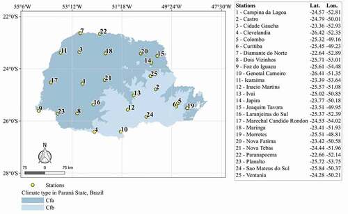
The present study was carried out for the Paraná State (), sub-tropical region of Southern Brazil, with an area of 199 307 922 km2 and predominance Cfa and Cfb climate types, according to Maack (Citation2012). The Cfa sub-tropical climate has a good rainfall distribution, with an average 1500 mm year–1, and an average annual temperature of 19°C. The Cfb sub-tropical climate presents rainfall of more than 1200 mm year–1, well distributed throughout the year, and a temperate summer, with an annual average temperature of 17°C (Alvares et al. Citation2013).
Figure 1. Predominant climate types in Paraná State and location of weather stations. Source: Adapted from Paraná Agronomic Institute (IAPAR Citation2019); adapted from de Brazilian Institute of Geography and Statistics (IBGE Citation2010)
2.2 Weather data used
Data series from 25 automatic weather stations () were used, obtained from the National Institute of Meteorology (INMET), covering the period from 1 December 2016 to 8 November 2018.
The following climate data were required to estimate the hourly and daily ETo with the ASCE-PM (EToh and ETod, respectively) model: maximum and minimum air temperatures (T; °C); maximum and minimum relative humidity (RH; %); incident solar radiation (Rs; MJ m–2 h–1); and wind speed at 10 m height (u10; m s–1), which was later converted to 2 m height (u2; m s–1) at an hourly scale (Allen et al. Citation1998).
The total number of hours analysed is 424 800, or 2 548 800 data points in total (6 variables × 424 800 h = 2 548 800 data), for the 25 stations analysed. However, it was decided to exclude periods with climatic input variable that presented failure on readings data to estimate ETo, as well as out-of-normal values or outliers. With this data correction, 331 344 hours or 1 988 064 data were effectively used in the EToh and EToMJS.h calculations, representing a 22% reduction in the total hours.
2.3 Estimation of reference evapotranspiration (ETo) at the hourly scale
The estimation of hourly ETo (EToh; standard) was performed with the standardized Penman-Monteith equation (EquationEquation (1)(1)
(1) ), presented by the American Society of Civil Engineers (ASCE-EWRI Citation2005), using a short crop height of 0.12 m.
where EToh is the reference evapotranspiration at each i hour (mm h–1); Δ is the slope of the saturated water–vapour–pressure curve to the air temperature in the period considered (kPa °C–1); 0.408 is the inverse value of the latent heat of vaporization (λ = 2.45 MJ kg–1); Rn is the net radiation balance in the period considered (MJ m–2 h–1); G is the soil heat flux in the period considered (MJ m–2 h–1); γ is the psychrometric constant (kPa °C–1); Cn is the constant related to the type of vegetation and time scale considered (Cnhourly = 37 K mm s3 Mg–1 h–1 for soil cover with short grass); T is the average air temperature in the period considered (°C); u2 is the wind speed at 2 m height in the period considered (m s–1); es is the saturation vapour pressure in the period considered (kPa); ea is the actual vapour pressure in the period considered (kPa); and Cd is the constant related to the type of vegetation and time scale (considered Cddaytime = 0.24 s m–1 for daytime period and short grass, or Cdnighttime = 0.96 s m–1 for night-time period and short grass).
The hourly EToMJS.h was calculated using the MJS model, which considers only the atmospheric water potential Ψair (EToMJS as a function of Ψair; EquationEquations (2)(2)
(2) and (Equation3
(3)
(3) )):
where EToMJS.h is the reference evapotranspiration estimated with the atmospheric water potential (mm h–1); a is the linear coefficient obtained from the linear regression equation, resulting from the relation between Ψairh and EToh (mm h–1); b is the angular coefficient obtained in the linear regression equation, resulting from the relation between Ψairh and EToh (mm h–1 MPa–1; MPa is megapascal); Ψairh is the atmospheric water potential at each i hour (MPa); R is the gas constant (8.314 J mol−1 K−1); T is the average air temperature in the period considered (K); Mv is the partial molar volume of water (18.10–6 m3 mol–1); ea is the actual vapour pressure in the period considered (MPa); and es is the saturation vapour pressure in the period considered (MPa).
The analysis with the model that estimates EToMJS.h was carried out in two stages:
(i) The first stage, according to Jerszurki et al. (Citation2017), consisted in calculating the values for the Ψairh (EquationEquation (3)(3)
(3) ) and EToh (EquationEquation (1)
(1)
(1) ) series. Then the calibration was performed by a simple linear regression analysis between Ψairh and EToh, to obtain the a and b coefficients to use in EquationEquation (2)
(2)
(2) to estimate the EToMJS.h. Calibration was performed for 25 weather stations analysed in Paraná State, considering the climate data for the period from 1 December 2016 to 1 December 2017.
(ii) The second stage consisted in analysing the performance of the method that estimates EToMJS.h (EquationEquation (2)(2)
(2) ), performing a correlation between EToMJS.h and EToh. Validation analyses were performed for 25 weather stations tested in Paraná State, considering the climate data for the period from 2 December 2017 to 8 November 2018.
2.4 Estimation of reference evapotranspiration (ETo) at the daily scale
The reference evapotranspiration estimates at the daily scale with the MJS, HS (Hargreaves and Samani Citation1985), PET (Tegos et al. Citation2017) and PMT methods were compared with the estimates performed by the ASCE-PM method. The estimation was performed for 24 weather stations in the Paraná State, considering the climate data for the period from 2 December 2017 to 8 November 2018.
The methods ASCE-PM (EToh; EquationEquation (1)(1)
(1) ) and MJS (EToMJS.h; EquationEquations (2)
(2)
(2) and (Equation3
(3)
(3) )), calculated at the hourly scale, had the ETo of the 24 hours of the day added to compose the daily values: ETod and EToMJS.d, respectively. The HS and PET methods were calculated using EquationEquations (4)
(4)
(4) and (Equation5
(5)
(5) ). The PMT method was calculated with EquationEquation (1)
(1)
(1) , using as input, for each location, the maximum and minimum daily temperatures and the average normal wind speed at 2 m height (Raziei and Pereira Citation2013, Paredes et al. Citation2020a, Citation2020b). As the areas analysed have a humid climate (Cfa and Cfb), the Tdew was considered equal to [Tmean – 2°C] (Paredes et al. Citation2020b), and the incident solar radiation (Rs) was estimated with the Hargreaves and Samani equation (EquationEquation (6)
(6)
(6) ), adopting the coefficient KRs = 0.16°C–5, characteristic of inland sites proposed in FAO 56 (Allen et al. Citation1998).
where EToHS.d is the evapotranspiration at each i day, estimated with the Hargreaves and Samani equation (mm day–1); PETd is the potential evapotranspiration at each i day, estimated with the modified parametric model (mm day–1; Tegos et al. Citation2017); RsHS is the daily shortwave solar radiation (MJ m−2 d–1) directly expressed as influenced by KRs (°C–5), required in the calculation of the PMT; λ is the latent heat of vaporization (2.45 MJ kg–1); Ra is the extraterrestrial radiation (MJ m–2 day–1); T is the temperature (°C), which can be maximum, minimum or medium; and a’ and c’ are the parameters of PET equation. The extraterrestrial radiation (Ra) was calculated according to Allen et al. (Citation1998).
The parameters a’ and c’ of the PET equation were obtained using the inverse distance weighted (IDW) method, in the R software. Values of a’ and c’ obtained from Tegos et al. (Citation2017) for the Paraná State (Maringá: a’ = 0.0000875 and c’ = 0.0037; Curitiba: a’ = 0.0000570 and c’ = 0.0153; and Ponta Grossa: a’ = 0.0000547 and c’ = 0.0166) were interpolated and extrapolated to the entire state.
2.5 Statistical analysis for comparison
The values of hourly and daily ETo obtained with the MJS (EToMJS.h and EToMJS.d), HS (EToHS.d), PET (EToPET.d), PMT (EToPMT.d) and ASCE-PM (EToh and ETod) methods were compared and verified in linear regression analysis, as well as the main error (root mean square error), index (Willmott’s “d” agreement) and coefficient (Pearson’s r correlation) recommended in the literature (Jacovides and Kontoyiannis Citation1995) and the model efficiency (Nash and Sutcliffe Citation1970):
where RMSE is the root mean square error (mm period–1); r is the Pearson correlation coefficient (dimensionless); d is the agreement index of Willmott (Citation1982) (dimensionless); NSE is the Nash-Sutcliffe model efficiency (dimensionless); is the reference evapotranspiration estimated with the standard ASCE-PM method at each i period (mm period–1);
is the reference evapotranspiration estimated with the alternative approach (MJS, HS, PET, PMT) at each i period (mm period–1); n is the number of days or hours analysed (dimensionless);
is the mean reference evapotranspiration estimated with the standard ASCE-PM method (mm period–1); and
is the mean reference evapotranspiration estimated with the alternative approach (MJS, HS, PET or PMT; mm period–1). The period considered varies according to the time scale (hourly or daily).
3 Results and discussion
3.1 Estimation of reference evapotranspiration (ETo) at the hourly scale
Twenty-five weather stations were analysed between 1 December 2016 and 8 November 2018, 15 in the Cfa climate type and 10 in Cfb. Air temperature (T), relative humidity (RH), incident solar radiation (Rs) and wind speed at 2 m height (u2) in general showed very similar trends among the predominant climates of Paraná (). It was observed that: (i) T was higher in the spring (approximately 20°C for Cfa climate and 18°C for Cfb) and summer (24°C for Cfa and 19°C for Cfb); (ii) RH showed no high seasonal variations for either climate, being between 66% and 80% throughout the year, with winter displaying the lowest RH for Cfa (66%) and summer for Cfb (74.9%); (iii) Rs showed a similar trend to T, with higher Rs periods in the spring (0.84 MJ m2 h–1 for Cfa and 0.75 MJ m2 h–1 for Cfb) and summer (0.95 MJ m2 h–1 for Cfa and 0.94 MJ m2 h–1 for Cfb); and (iv) u2 showed a similar trend to RH, with little seasonal variation, being between 0.95 and 1.45 m s–1, with the highest values observed during the autumn period (1.45 m s–1 for Cfa and 1.36 m s–1 for Cfb).
Figure 2. Seasonal average variation of the climatic variables of 15 and 10 weather stations in Cfa and Cfb climate types, respectively, in Paraná State, for the period 1 December 2016 to 8 November 2018: (a) air temperature (T; °C); (b) relative humidity (RH; %); (c) incident solar radiation (Rs; MJ m–2 h–1); (d) wind speed at 2 m height (u2; m s–1)
3.2 Calibration of the MJS model to obtain “a” and “b” parameters
As the hourly values of ETo are low, the “a” parameters (linear coefficient of the MJS model) were between −0.0079 and 0.0328 mm h–1 for Cfa climate, and between −0.024 and 0.026 mm h–1 for Cfb climate (). The “b” parameters (angular coefficient of the MJS model) were between −6.96E-09 and −2.61E-09 mm h–1 MPa–1 for locations with Cfa climate, and between −5.59E-09 and −2.9E-09 mm h–1 MPa–1 for Cfb. The coefficients obtained in the correlation between Ψairh and EToh were not as narrow as those obtained by Oliveira (Citation2018), at the hourly scale, for Cfa (0.81 ≤ r ≤ 0.96) and Cfb (0.84 ≤ r ≤ 0.90) climates. However, Oliveira (Citation2018) performed linear and quadratic adjustments in their analyses. The range of correlation coefficients in this study is wider and lower than those obtained by Oliveira (Citation2018) due to the longer period analysed here. In the present study, in addition to making only linear adjustments, a one-year hourly data period was used, whereas Oliveira (Citation2018) used only two months of hourly data in their calibration analyses. Thus, removing the Campina da Lagoa station (r = 0.37), the correlation coefficients were 0.51 ≤ r ≤ 0.77 for locations with Cfa climate, and 0.58 ≤ r ≤ 0.78 for locations with Cfb climate.
Table 1. Calibration of the MJS model for 25 weather stations located in Cfa and Cfb climate types, in Paraná State, for the period 1 December 2016 to 1 December 2017: linear coefficient (“a”); angular coefficient (“b”); correlation coefficient (r); and number of data in the analyses (n)
The results of calibration performed with the MJS model in the present study are consistent with those obtained by Jerszurki et al. (Citation2017) at the daily scale, and with Oliveira (Citation2018) at daily and hourly scale. There is evidence that the MJS model has less sensitivity in humid sub-tropical climates, due to the small range between the lowest and highest value of the atmospheric water potential (Ψair). The lower range, or amplitude, is due to the lower temperatures and higher RH values (Jerszurki et al. Citation2017). All of these aspects contributed to the fact that the correlation coefficient (r) values were not so narrow in the correlation between Ψairh and EToh, as was verified in arid and semi-arid climates (Jerszurki et al. Citation2017, Oliveira Citation2018). In addition, the number of data used in the regression analysis for each location was very high (4045 ≤ n ≤ 8614; ), which increases variability and generally tends to reduce the values of r when working with climate data.
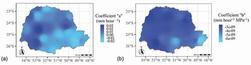
With the values of the parameters “a” and “b” of the MJS model for each one of the 25 weather stations analysed in the Paraná State, the results were interpolated and a map of the parameters values was developed (). Once established, the coefficients “a” and “b” from each type of climate can be extrapolated to locations that present the same climatic characteristics, without requiring new calibrations.
Figure 3. Spatialization of “a” and “b” coefficients of the Moretti-Jerszurki-Silva model, in Paraná State: (a) linear coefficient (“a”; mm h–1); (b) angular coefficient (“b”; mm h–1 MPa–1)
3.3 Validation of the MJS model: variation and correlation between EToMJS.h and EToh in Paraná State
The Cfa and Cfb climates showed similar trends between the EToMJS.h and EToh methods. There was no considerable variation in the values of ETo (EToMJS.h and EToh) between seasons. In the autumn period there were many input data errors (lack of data), and therefore, this seasonal period was not evaluated. Similarly, the months of February and March showed many failures in input data and, for this reason, these months were also not analysed ( and ).
Table 2. Seasonal averagesa of EToMJS.h and EToh (mm h–1) of 25 weather stations in Paraná State, for the period 2 December 2017 to 8 November 2018
Figure 4. Averages of EToMJS.h and EToh, at the hourly scale, from weather stations according to the Cfa and Cfb climate types, in Paraná State, for the period 2 December 2017 to 8 November 2018: (a) seasonal average; (b) monthly average
The averages of EToMJS.h and EToh for the seasonal and monthly periods were very close () and (b)). The highest amplitudes between EToMJS.h and EToh occurred in the winter, a period in which the RH remains high and the values of T were lower. Jerszurki et al. (Citation2017) and Oliveira (Citation2018), analysing the MJS model as a function of only Ψair, for several Brazilian climate types, also found that the model performance worsened in these conditions – in other words, for colder and wetter climates or periods. The highest discrepancies occurred in Dois Vizinhos and Nova Tebas cities for Cfa climate, and in Clevelândia for Cfb climate.
In the validation process of the 25 locations in Paraná State, excluding the autumn period (all locations) and Clevelândia and Nova Tebas stations, due to problems with the climatic data, the following statistical indicators of the MJS model were found in the correlation between EToMJS.h and EToh ():
The correlation coefficients (r) were lower in winter for Cfa (0.53 ≤ r ≤ 0.82) and Cfb (0.81 ≤ r ≤ 0.84) climates, and higher in summer and spring for Cfa (0.69 ≤ r ≤ 0.93) and Cfb (0.91 ≤ r ≤ 0.93);
The NSE was higher in the spring (–2.29 ≤ NSE ≤ 0.82) and lower in the winter (–13.90 ≤ NSE ≤ 0.49) for Cfa climate. Disregarding autumn, due to the lack of data, it was found in the Cfb climate that the mean value observed was a better predictor than the simulated value.
The “d” index, which measures the proximity of the associated values in relation to the 1:1 line, also indicated lower values in winter for both Cfa (0.38 ≤ d ≤ 0.89) and Cfb (0.54 ≤ d ≤ 0.89) climates, and higher values in summer and spring for Cfa (0.5 ≤ d ≤ 0.95) and Cfb (0.73 ≤ d ≤ 0.97).
On average, the RMSE values obtained were also low. By season, winter also showed the highest errors for Cfa (0.02 ≤ RMSE ≤ 0.13) and Cfb (0.02 ≤ RMSE ≤ 0.9) climates, whereas the error was lower in summer and spring for Cfa (0.02 ≤ RMSE ≤ 0.14) and Cfb (0.02 ≤ RMSE ≤ 0.06).
Table 3. Seasonala and annual values of Nash-Sutcliffe efficiency (NSE; dimensionless), “d” index (dimensionless), root mean square error (RMSE; mm h–1) and correlation coefficient (r; dimensionless) between EToMJS.h and EToh, of 15 and 10 weather stations in Cfa and Cfb climate types, respectively, in Paraná State, for the period 2 December 2017 to 8 November 2018
In general, it was found that EToMJS.h presented higher values on average than EToh at night-time () and (c)). With the sunrise, EToh became progressively higher than the EToMJS.h. Considering the input variables in both models (MJS and ASCE-PM), the results are consistent. T and RH are considered directly or indirectly in both methodologies. The ASCE-MP method considers Rs and u2 while the MJS method does not. Thus, at night-time there are no Rs and the u2 is low, providing lower values of ETo. During the day, the opposite occurs, considering that Rs and u2 are higher, favouring higher values of ETo.
Figure 5. Variation and correlation between EToMJS.h and EToh, at the hourly scale, of 15 and 10 weather stations in Cfa and Cfb climate types, respectively, in Paraná State, for the period 2 December 2017 to 8 November 2018: (a) hourly ETo without delay adjustment, in Cfa climate; (b) hourly ETo with 2-h delay adjusted, in Cfa climate; (c) hourly ETo without delay adjustment, in Cfb climate; (d) hourly ETo with 2-h delay adjusted, in Cfb climate
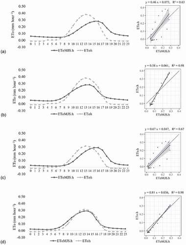
In checks of all daily and average trends () and (c)) of the hourly ETo, for 25 weather stations in Paraná State (Cfa and Cfb climates), we found the existence of a delay on the maximum ETo point obtained with the two methodologies (MJS and ASCE-PM). For the ASCE-PM model, the maximum EToh occurred at between 12:00 and 14:00 hours (except for Clevelândia station), the time when the highest values of incident solar radiation are generally observed. For the MJS model, the maximum EToMJS.h occurred between 14:00 and 16:00 hours () and (c)), a period in which the highest temperatures of the day and the lowest relative humidity generally occur. This aspect is interesting and deserves to be investigated. On average, there was a delay of approximately two hours delay in the curve of the hourly ETo value throughout the day, estimated using both methodologies () and (c)).
Although the statistical results shown in are very promising, the delay in the values of ETo estimated with both methodologies (MJS and ASCE-PM) certainly limited the statistical measures used to verify the validation process of the correlation between EToMJS.h and EToh (). Thus, correcting the hours and analysing the effect of the delay on ETo estimates can lead to better and more promising statistical indicators for an alternative method as simple as the MJS, to estimate hourly ETo.
The correction of the two-hour delay between EToMJS.h and EToh on all days, at the 25 stations analysed in Paraná State, provided an average trend as shown in ) and (d). With the correction, the occurrence time of maximum ETo estimated with the MJS model started to coincide with the ASCE-PM methodology. With the adjustment made, there was an improvement in the correlation between EToMJS.h and EToh ().
Figure 6. Indexes and errors before and after the correction of the delay observed in the correlation between EToMJS.h and EToh, at the hourly scale, of 25 weather stations, 15 and 10 in climate types Cfa and Cfb, respectively, in Paraná State, for the period 2 December 2017 to 8 November 2018: (a) Nash-Sutcliffe efficiency (NSE; dimensionless); (b) root mean square error (RMSE; mm day–1); (c) correlation (r; dimensionless)
The existence of a delay between the values of EToMJS.h and EToh for Cfa and Cfb climates, in Paraná State, generated uncertainty regarding the existence of a similar trend for the ETo estimated with the two methodologies for the main climates in Brazil (Af, Am, Aw, BSh; Cfa, Cfb, Cwa and Cwb). This is an important aspect and will need to be investigated in more detail later, considering the findings obtained in the present study and the conclusions of Oliveira (Citation2018). It would be interesting to verify the magnitude and time of occurrence of the highest and lowest hourly values of ETo estimated with the ASCE-PM and MJS methodologies, as well as the existence and cause of delays in the trends of the estimated values for EToMJS.h and EToh.
3.4 Estimation of reference evapotranspiration (ETo) at the daily scale
In the analysed period (2 December 2017 to 8 November 2018), not all alternative approaches tested (MJS, HS, PET and PMT) showed average values of daily ETo very close to those obtained with the standard ASCE-PM model (). The average values of daily ETo estimated for the 24 weather stations in the Paraná State were interpolated and presented on maps (). The location of Clevelândia was excluded from the analyses as it had a lot of missing data.
Table 4. Average daily values of reference evapotranspiration (ETo; mm day–1) of 24 weather stations in Paraná State, for the period 2 December 2017 to 8 November 2018
Figure 7. Daily reference evapotranspiration (ETo; mm day–1) of 24 weather stations in Paraná State, obtained with the inverse distance weighting (IDW) method, for the following models: (a) ASCE-PM (ETod); (b) Moretti-Jerszurki-Silva (EToMJS.d); (c) Hargreaves and Samani (EToHS.d); (d) modified parametric (EToPET.d); and (e) Penman-Monteith temperature (EToPMT.d)
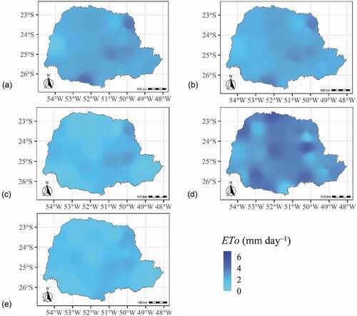
The indexes, errors and statistical coefficients indicated better performance of the MJS model in the 24 locations and climates (Cfa and Cfb) analysed in the Paraná State (). Although the values of EToMJS.d resulted from the 24-hour sum, as in the ASCE-PM (ETod), it is believed that the calibration of the “a” and “b” coefficients of the model contributed substantially to improving the performance. The result is interesting, since Jerszurki et al. (Citation2017) considered that the MJS model presents good results at the daily scale, with lower performance in regions with higher RH and low temperatures, as occurs in Cfa and Cfb climates. Therefore, there is an expectation that the spatialization of EToMJS.d in hot and dry regions will be even better.
Table 5. Daily values of Nash-Sutcliffe efficiency (NSE), root mean square error (RMSE) and correlation coefficient (r; dimensionless) in the correlations between “EToMJS.d and ETod,” “EToHS.d and ETod,” “EToPET.d and ETod” and “EToPMT.d and ETod” of 15 and nine weather stations in Cfa and Cfb climate types, respectively, in Paraná State, for the period 2 December 2017 to 8 November 2018
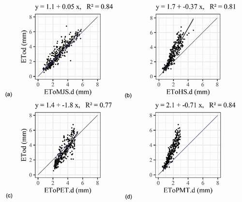
The statistical results of the HS method () did not indicate good performance in some locations, mainly in Dois Vizinhos, Diamante do Norte, Icaraíma, Japirá and Colombo. The HS and PMT models underestimated the values of daily ETo in relation to the ASCE-PM model for Cfa climate. For Cfb, the HS model had the highest underestimation in relation to all tested models ( and ). Several locations presented NSE < 0, indicating that the average values of ETod (ASCE-PM) result in better prediction than the HS model (EToHS.d). The opposite results were observed by Todorovic et al. (Citation2013), which in Mediterranean climates observed overestimation of ETo with the HS method in relation to the standard ASCE-PM. As the HS method does not consider the relative humidity, which has high value for Cfa and Cfb climates, the method was less accurate in humid climates, with low performance in relation to the other analysed methods.
There was an overestimation of the daily values of ETo with the PET model in relation to the ASCE-PM model ( and ), in Cfa and Cfb climates, indicating less efficiency for the sub-tropical region of Brazil. In addition, 16 locations presented NSE < 0. The lowest efficiencies (NSE) occurred in Morretes, Joaquim Távora, Ventania, Ivaí, São Mateus do Sul and Inácio Martins (). The few parameters a’ and c’ available for IDW extrapolation may have contributed to the model’s low performance. However, Tegos et al. (Citation2017), evaluating evapotranspiration with the PET model for 4088 stations worldwide, also found less precision with the model in the equatorial regions of South America, Africa, Indonesia and the Indian Peninsula. The authors considered that the poor performance was probably because the model does not account for the relative humidity and wind speed. The two variables are not considered in the PET model, but are very active in the evapotranspiration process in the mentioned areas, influencing the net solar radiation and the evaporation demand.
The PMT model underestimated the ETod, presenting results similar to the HS model for the Cfa climate. However, in the Cfb climate, the PMT was not the model that had the lowest underestimations in relation to the ASCE-PM (; ). Considering the 1:1 line, PMT and HS () and (d)) also produced similar results, presenting the lowest adjustment and performance in the analyses () for the sub-tropical region of Brazil.
Figure 8. Simple linear regression analysis of the values of daily reference evapotranspiration (ETo; mm day–1) of 24 weather stations in Paraná State, for the period 2 December 2017 to 8 November 2018, for the correlation between: (a) EToMJS.d and ETod; (b) EToHS.d and ETod; (c) EToPET.d and ETod; (d) EToPMT.d and ETod
4 Conclusions
In the calibration, the “a” coefficients of the MJS model were between −0.0133 and 0.0328 mm h–1 for Cfa climate, and between −0.024 and 0.026 mm h–1 for Cfb climate. The “b” parameters were between −6.96E-0.9 and −2.46E-0.9 mm h–1 MPa–1 for Cfa climate, and between −5.53E-0.9 and −2.99E −0.9 mm h–1 MPa–1 for Cfb climate.
The values of EToMJS.h are higher than EToh at night-time. With the sunrise, the opposite occurs, and the EToh becomes progressively higher than EToMJS.h.
The curve of hourly ETo value, estimated using the ASCE-PM and MJS methodologies, presents, on average, a two-hour delay between the maximum values of hourly ETo throughout the day. The correction of the two-hour delay improved the EToMJS.h estimates in relation to EToh for Cfa and Cfb climates, in Paraná State.
On average, the values of EToMJS.h and EToh were close and well associated statistically in Paraná State. The highest amplitudes and less narrow correlations occurred in the winter season, a period when the RH remains high and the values of T are lower. Summer and spring had equivalent values of EToMJS.h and EToh, with smaller amplitudes and closer correlations.
The Moretti-Jerszurki-Silva alternative approach showed better efficiency in relation to the Hargreaves and Samani, modified parametric and Penman-Monteith temperature models, being the best alternative methodology to produce accurate evapotranspiration estimates at a daily scale, for Cfa and Cfb climate types, in the sub-tropical region of Brazil.
Disclosure statement
No potential conflict of interest was reported by the author(s).
References
- Allen, R.G., et al., 1998. Crop evapotranspiration - guidelines for computing crop water requirements. Irrigation and Drainage Paper 56. Rome: FAO. Available from: http://www.fao.org/3/x0490e/x0490e00.htm [Accessed 18 February 2019].
- Alvares, C.A., et al., 2013. Köppen’s climate classification map for Brazil. Meteorologische Zeitschrift, 2, 11–728. doi:https://doi.org/10.1127/0941-2948/2013/0507
- Alves Sobrinho, T., et al., 2011. Estimativa da evapotranspiração de referência através de redes neurais artificiais. Revista Brasileira de Meteorologia, 26 (2), 197–203. doi:https://doi.org/10.1590/S0102-77862011000200004
- ASCE-EWRI, 2005. The ASCE standardized reference evapotranspiration equation. Report of the Task Committee on Standardization of Reference Evapotranspiration. Reston: American Society of Civil Engineers. doi:https://doi.org/10.1061/40499(2000)126
- Fenner, W., et al., 2019. Development, calibration and validation of weighing lysimeters for measurement of evapotranspiration of crops. Revista Brasileira de Engenharia Agrícola e Ambiental, 23 (4), 297–302. doi:https://doi.org/10.1590/1807-1929/agriambi.v23n4p297-302
- Hargreaves, G.H. and Samani, Z.A., 1985. Reference crop evapotranspiration from temperature. Applied Engineering in Agriculture, 1 (2), 96–109. doi:https://doi.org/10.13031/2013.26773
- Hillel, D., 1971. Soil and water: physical principles and processes. New York: Academic press.
- IAPAR, 2019. Paraná Agronomic Institute [online]. Download of shapefile containing the prevailing climatic classification of Paraná State. Available from: http://www.iapar.br/ [Accessed 15 November 2019].
- IBGE, 2010. Brazilian Institute of Geography and Statistics [online]. Download of shapfile concerning the cities of Paraná State. Available from: ftp://geoftp.ibge.gov.br/cartas_e_mapas/mapas_para_fins_de_levantamentos_estatisticos/censo_demografico_2010/mapas_municipais_estatisticos/ [Accessed 15 November 2019].
- Jacovides, C.P. and Kontoyiannis, H., 1995. Statistical procedures for the evaluation of evapotranspiration computing models. Agricultural Water Management, 27, 365–371. doi:https://doi.org/10.1016/0378-3774(95)01152-9
- Jerszurki, D., Souza, J.L.M., and Silva, L.C.R., 2017. Expanding the geography of evapotranspiration: an improved method to quantify land-to-air water fluxes in tropical and subtropical regions. PloS One, 12 (6), e0180055. doi:https://doi.org/10.1371/journal.pone.0180055
- Maack, R., 2012. Geografia física do Estado do Paraná. 4th ed. Curitiba: IBPT.
- Maina, M.M., et al., 2014. Effects of crop evapotranspiration estimation techniques and weather parameters on rice crop water requirement. Australian Journal of Crop Science, 8 (4), 495–501. Available from: http://www.cropj.com/maina_8_4_2014_495_501.pdf [Accessed 30 May 2019].
- Moura, A.C., et al., 2013. Evapotranspiração de referência baseada em métodos empíricos em bacia experimental no Estado de Pernambuco - Brasil. Revista Brasileira de Meteorologia, 28 (2), 181–191. Available from: http://www.scielo.br/pdf/rbmet/v28n2/v28n2a07.pdf [Accessed 20 March 2019].
- Nash, J.E. and Sutcliffe, J.E., 1970. River flow forecasting through conceptual models: part I. A discussion of principles. Journal of Hydrology, 10 (3), 282–290. doi:https://doi.org/10.1016/0022-1694(70)90255-6
- Nolz, R. and Rodný, M., 2019. Evaluation and validation of the ASCE standardized reference evapotranspiration equations for a subhumid site in northeastern Austria. Journal of Hydrology and Hydromechanics, 67, 289–296. doi:https://doi.org/10.2478/johh-2019-0004
- Oliveira, S.R., 2018. Ajuste do método Moretti-Jerszurki-Silva para estimar a evapotranspiração de referência diária e horária dos tipos climáticos brasileiros. Thesis (PhD). Federal University of Paraná. Available from: http://www.moretti.agrarias.ufpr.br/publicacoes/tese_2018_oliveira_s_r.pdf [Accessed 12 January 2019].
- Owusu-Sekyere, J.D., Ampofo, E.A., and Asamoah, O., 2017. Comparison of five different methods in estimating reference evapotranspiration in Cape Coast, Ghana. Academic Jounals. African Journal Agricultural Research, 12 (40), 2976–2985. doi:https://doi.org/10.5897/AJAR2017.12594
- Paredes, P., et al., 2020a. Daily grass reference evapotranspiration with Meteosat Second Generation shortwave radiation and reference ET products. Agricultural Water Management, 248 (106543), 1–20. doi:https://doi.org/10.1016/j.agwat.2020.106543
- Paredes, P., et al., 2020b. Reference grass evapotranspiration with reduced data sets: parameterization of the FAO Penman-Monteith temperature approach and the Hargeaves-Samani equation using local climatic variables. Agricultural Water Management, 240 (106210), 1–23. doi:https://doi.org/10.1016/j.agwat.2020.106210
- Philip, J.R., 1964. Sources and transfer processes in the air layers occupied by vegetation. Journal of Applied Meteorology, 3 (4), 390–395. doi:https://doi.org/10.1175/1520-0450(1964)003<0390:SATPIT>2.0.CO;2
- Raziei, T. and Pereira, L.S., 2013. Estimation of ETo with Hargreaves–Samani and FAO-PM temperature methods for a wide range of climates in Iran. Agricultural Water Management, 121, 1–18. doi:https://doi.org/10.1016/j.agwat.2012.12.019
- Tegos, A., et al., 2017. Parametric modelling of potential evapotranspiration: a global survey. Water, 9 (795), 1–22. doi:https://doi.org/10.3390/w9100795
- Tegos, A., Efstratiadis, A., and Koutsoyiannis, D., 2013. A parametric model for potential evapotranspiration estimation based on a simplified formulation of the Penman-Monteith equation. InTech, 143–165. doi:https://doi.org/10.5772/52927
- Tegos, A., Malamos, N., and Koutsoyiannis, D., 2015. A parsimonious regional parametric evapotranspiration model based on a simplification of the Penman–Monteith formula. Journal of Hydrology, 524, 708–717. doi:https://doi.org/10.1016/j.jhydrol.2015.03.024
- Todorovic, M., Karic, B., and Pereira, L.S., 2013. Reference evapotranspiration estimate with limited weather data across a range of Mediterranean climates. Journal of Hydrology, 481, 166–176. doi:https://doi.org/10.1016/j.jhydrol.2012.12.034
- Treder, W. and Klamkowski, K., 2017. An hourly reference evapotranspiration model as a tool for estimating plant water requirements. Infrastruktura i ekologia terenów wiejskich infrastructure and ecology of rural areas, 2, 469–481. doi:https://doi.org/10.14597/infraeco.2017.2.1.035
- Willmott, C.J., 1982. Some comments on the evaluation of model performance. Bulletin American Meteorology Society, 63, 1309–1313. doi:https://doi.org/10.1175/1520-0477(1982)063<1309:SCOTEO>2.0.CO;2
- Yildirim, Y.E., et al., 2004. Comparison of hourly and daily reference evapotranspiration vaues for GAP project area. Journal of Applied Sciences, 4, 53–57. doi:https://doi.org/10.3923/jas.2004.53.57