Assessing different roles of baseflow and surface runoff for long-term streamflow forecasting in southeastern China

ABSTRACT

Accurate long-term streamflow forecast is essential to alleviate and solve the water security problems related to flood and drought disaster warnings. In this study, a new strategy for forecasting monthly streamflow is proposed and four scenarios are designed for the evaluation of different roles of baseflow and surface runoff on performances of long-term streamflow forecasting. The developed models are evaluated at multiple streamflow sites located in the Zhejiang Province of China. The results show that artificial intelligence (AI)-based models with two predictor variables (i.e. baseflow and surface runoff) performed better than that with a single predictor (streamflow) for all the months in a year, and the prediction accuracy of annual peak and monthly streamflow values is improved. Based on the comprehensive evaluations of all the models, the baseflow and surface runoff values are recommended as inputs to AI-based models for an improved prediction accuracy of streamflows.

KEYWORDS:

• long-term streamflow forecast
• baseflow
• surface runoff
• AI-based models
• forecast performance

Editor A. Fiori Associate editor M. Ionita

1 Introduction

The development of streamflow forecasting models with high prediction accuracy has always been an essential task for water resources and disaster management. Typically, hydrological forecasting can be divided into short-term and long-term predictions; the lead time of the former is within 72 hours, while that of the latter is greater than or equal to one month. Streamflow forecasts are critical for flood and drought disaster management (Sattari et al. 2012, Turner et al. 2017, Kao et al. 2020), safe and economic operation of reservoirs (Block 2011, Humphrey et al. 2016, Yang et al. 2017, Zhang et al. 2018), and optimal allocation of water resources (Mendoza et al. 2017, Kratzert et al. 2018, Tan et al. 2018). Several studies have reported the use of long-term streamflow forecasting models in major basins around the world in recent years, such as the Yangtze River (China) (Zhou et al. 2018), Yellow River (China) (Wang et al. 2018), Mahanadi River (India) (Sahoo et al. 2019), South Korean basins (Ajmal et al. 2015), eastern Australia basins (Loveridge et al. 2017), Sicilian River (Italy) (Pumo et al. 2016), and Gediz Basin (Turkey) (Turan and Yurdusev 2014).

Long-term streamflow forecasting models can be classified as physics-based and data-driven models. The latter do not consider the physical mechanisms and processes responsible for streamflow generation. Data-driven models include time series analysis (Cooper et al. 2018, Papacharalampous and Tyralis 2020, Kim et al. 2021), regression-based models (Fashae et al. 2019, Zuo et al. 2020), artificial neural networks (ANNs) (Cheng et al. 2020a, Hassan and Hassan 2020, Lv et al. 2020), and support vector machines (SVMs) (Bhandari 2019, Yu et al. 2020). The time series models are based on historical observations of hydrological elements to explore their evolution to forecast the hydrological processes, such as the autoregressive moving average (ARMA) model (Box and Jenkins 2010) and autoregressive integrated moving average (ARIMA) model (Carlson et al. 1970). Regression analysis is a method that considers the changes in the predicted objects due to the influencing factors. The ANN is a nonlinear system composed of many neurons, which has excellent self-learning and self-adaptive performance, and is widely used in streamflow and precipitation forecasting (Li et al. 2019), including the long short-term memory (LSTM) model, gated recurrent unit (GRU) model, and back-propagation (BP) model. An SVM is a generalized linear classifier that classifies data according to supervised learning, and its decision boundary is the maximum margin hyperplane (Zhu et al. 2016).

Several long-term streamflow forecasting models are commonly used for flood and drought management, but those models still have much room for improvement in their forecasting accuracy. Furthermore, due to the influences of climate change, human activities, and the complexity of the hydrological process itself, these models cannot fully capture all the characteristics of hydrological processes. Data-driven forecasting models can be improved by incorporating variables that are linked to streamflow generating mechanisms and can help explain their variability in time. Ensuring the inclusion of causal variables (e.g. a variable that influences another variable) in data-driven models can help capture the physical mechanisms responsible for the behaviour of the predictand (i.e. streamflow).

To characterize the complete set of hydrological processes contributing to streamflow generation and improve the prediction accuracies of the models in long-term streamflow forecasts, baseflow and surface runoff are used and evaluated as predictor variables in multiple data-driven models in this study. Surface runoff is the water that immediately contributes to river flow after rainfall events, as quick flow. Baseflow is the less undulating part of the hydrograph when the river is in the dry season and is the primary source of water supply that helps maintain reasonable river flow conditions. Baseflow separation approaches that partition the streamflow into different components, such as the surface flow and subsurface flow (Ahiablame et al. 2013), can help estimate baseflow for use in data-driven models. Due to the differences in basin attributes, the estimates from baseflow separation methods may be different. Only a few studies (Corzo and Solomatine 2007, Tongal and Booij 2018, Huang et al. 2020) related to short-term streamflow forecasts have used both baseflow and surface runoff characteristics. There have been very few studies in long-term streamflow forecasting to use both baseflow and surface runoff as predictor variables, where baseflow can be a more important causal variable explaining the variations in streamflows.

Therefore, the main focus of this study is to evaluate the efficacy of data-driven forecasting models that use baseflow, surface runoff, and streamflow variables as inputs, and these models are evaluated for forecast skill and their utility for water resources management in this study. The three main objectives of this study are therefore: (1) to use an appropriate baseflow separation method to separate the streamflow into baseflow and surface runoff; (2) to evaluate the performance of different models in long-term streamflow forecasting; and (3) to test the forecast results of baseflow, surface runoff, and streamflow as different predictor variables in artificial intelligence (AI)-based models.

2 Methodology

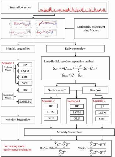
As an initial step of the forecasting model development, the existence or non-existence of trends in the available time series of streamflow needs to be evaluated using a non-parametric statistical hypothesis test (i.e. the Mann-Kendall (MK) test). Descriptions of the MK test and different AI-based models developed in this study are provided next. Figure 1 illustrates the methodology adopted in this study for forecasting monthly streamflow and evaluation of the models using four scenarios for different temporal and spatial scales.

Figure 1. Methodology using long-term streamflow forecasting models with four scenarios

2.1 Mann-Kendall test

The MK test is a rank-based nonparametric test that detects linear and nonlinear trends, where the null and alternative hypotheses are equal to the non-existence and existence of a trend in a time series, respectively (Mann 1945). The MK test has been used in several studies to evaluate the trend and stationarity analysis of meteorological and hydrological time series. When the test statistic (Z) used in the test provides a value of $\mathrm{Z}>0$, it can be concluded that the time series sequence shows an upward trend. When $\mathrm{Z}<0$, the time series represents a decreasing trend. The test can be conducted at a significance level of 5% to draw inferences about statistically significant trends. Climate change and human activities have a great impact on the regional hydrological process, and streamflow is becoming non-stationary. Trend analysis is important since the stationarity assessment is the premise of this study. Moreover, it can further illustrate the applicability of forecasting models when the streamflow series is stationary or non-stationary.

2.2 Forecasting models

2.2.1 Back-propagation neural network

The BP neural network is divided into input, hidden, and output layers, and the network layers are closely linked by weight bias. The BP prediction model is based on an error analysis between the training and expected results, and then the weight and thresholds are modified, step by step, to obtain a model that can produce output consistently with the desired results (Riad et al. 2004, Vivekanandan 2011). The algorithm of the BP long-term streamflow forecasting model consists of forward and backward propagation. In the forward propagation, the output $z$ of the $j$ neuron in the hidden layer is as shown below:

(1) $z_j=f\left(\sum _{i=1}^m{w}_{i,j}{x}_i+b_j\right)\mathrm{\forall }j$(1)

where $f\left(.\right)$ is the excitation function of neurons and $b_j$ represents bias. After the hidden layer mapping, $z_j$ is directly used as the input of the output layer, and the output layer is used for nonlinear fitting. At this point, the output $\widehat{Y_k}$ of the $k$ neuron in the output layer is:

(2) $\widehat{Y_k}=\sum _{i=1}^m{w}_{j,k}{z}_j+b_k\mathrm{\forall }k$(2)

where $b_k$ denotes bias from the hidden layer to the output layer. The error $e_k$ between measured and predicted streamflow is expressed as follows:

(3) $e_k=Y_k-\widehat{Y_k}\mathrm{\forall }k$(3)

where $Y_k$ indicates the expected output. The objective function of back-propagation is the sample mean square error $E$ of model training:

(4) $E=\frac{1}{2}{\left(Y_k-\widehat{Y_k}\right)}^2=\frac{1}{2}\sum _{k=1}^m{e}_k^2$(4)

BP neural network is an iterative learning algorithm that uses a gradient descent strategy to adjust the parameters with the target of a negative gradient direction in each iteration of back-propagation. The input layer to hidden layer weight $w_{i,j}$ and bias $b_k$ are updated to:

(5) $w_{i,j}=w_{i,j}+\eta H_j\left(1-z_j\right)x_i\sum _{k=1}^m{w}_{j,k}{e}_k\mathrm{\forall }i,j$(5)

(6) ${\mathrm{b}}_j={\mathrm{b}}_j+\eta z_j\left(1-z_j\right)\sum _{k=1}^m{w}_{j,k}{e}_k\mathrm{\forall }j$(6)

The weight of the hidden layer to the output layer $w_{j,k}$ and bias $b_k$ are renewed to:

(7) $w_{j,k}=w_{j,k}+\eta z_j{e}_k\mathrm{\forall }k$(7)

(8) ${\mathrm{b}}_k={\mathrm{b}}_k+\eta e_k\mathrm{\forall }k$(8)

2.2.2 LSTM network

LSTM is a unique recurrent neural network (RNN), which is divided into three layers with repeated chain structure (Werbos 1990, Hochreiter and Schmidhuber 1997). Compared with RNN, LSTM has a more complex system of its hidden layer, which adds a cell state and gate structure to control the flow of memory information and realize the long-term transmission and memory of knowledge. Hence, the LSTM model is more suitable for processing sequences with more extended time information than RNN and can carry long-term steps. The structure of the LSTM model mainly includes the following five parts:

1. The forgetting gate expression is as follows:

(9) $f_t=\sigma \left(W_f{h}_{t-1}+U_f{x}_t+b_f\right)$(9)

• (2) The input gate function is shown below:

(10) $i_t=\sigma \left(W_i{h}_{t-1}+U_i{x}_t+b_i\right)$(10)

• (3) The candidate gate expression is calculated as:

(11) $\stackrel{\sim }{C_t}\mathrm{t}\mathrm{a}\mathrm{n}\mathrm{h}\left(W_c{x}_t+U_c{h}_{t-1}+b_c\right)$(11)

• (4) The cell state renewal equation is expressed as:

(12) $C_t=f_t\times C_{t-1}+i_t\times \stackrel{\sim }{C_t}$(12)

• (5) The output gate function is calculated using the following equations:

(13) $O_t=\sigma \left(W_o{h}_{t-1}+U_o{x}_t+b_o\right)$(13)

(14) $h_t=O_t\times \mathrm{t}\mathrm{a}\mathrm{n}\mathrm{h}\left(C_t\right)$(14)

where $W_f$, $W_i$, $W_c$, and $W_o$ are the weight parameter matrix between the hidden layer forgetting, input, hidden candidate, and output gate and the upper layer neurons of the current time step; $U_f$, $U_i$, $U_c$, and $U_o$ represent the weight parameters between the input layer and forgetting, input, hidden candidate, and output gate; $b_f$, $b_i$, $b_c$, and $b_o$ denote the bias vectors of forgetting, input, hidden candidate, and output gate, respectively; $i_t$ indicates the output value of the input gate at the current time, is the bias of the input gate; $\mathrm{t}\mathrm{a}\mathrm{n}\mathrm{h}$ is the excitation function; and $h_t$ is defined as the output gate controlling the output state of cells.

2.2.3 GRU network

The GRU network simplifies the LSTM model in that it only retains the update gate and reset gate (Cho et al. 2014). GRU directly takes the long-term memory of a particular moment as the output and modifies the long-term memory while outputting. Therefore, GRU has fewer inputs than the LSTM network (LSTM has three inputs, whereas GRU has only two) and a more straightforward structure to reduce computation time. The GRU network combines the input gate and forgetting the gate into update gate $z$, cell state, and output gate into reset gate $r$. Reset and update gates are calculated as follows, where ⊙ is the Hadamard product:

(15) $r_t=\sigma \left(W^r{x}_t+U^r{h}_{t-1}\right)$(15)

(16) $z_t=\sigma \left(W^z{x}_t+U^z{h}_{t-1}\right)$(16)

where $x_t$ is the input of the current time step, $h_{t-1}$ represents information from the previous time step, $x_t$ and $h_{t-1}$ are zoomed via activation function to [−1,1]. Status information $h_t$ of the last time is shown below:

(17) $h_t=z_t\odot h_{t-1}+\left(1-z_t\right)\stackrel{\sim }{h_t}$(17)

The reset gate $r$ controls the information useful to $x_t$ in $h_t$, and then resets it. The equation for calculating the candidate hidden layer is as follows:

(18) $\stackrel{=}{h_t}\mathrm{t}\mathrm{a}\mathrm{n}\mathrm{h}\left(W_h{x}_t+U_h\left(r_t\odot h_{t-1}\right)\right)$(18)

where $r_t$ is the amount of information reserved in the previous period.

2.2.4 SVM model

The SVM approach uses a primary learning algorithm based on statistical learning knowledge, the structural risk minimization principle, and the dual idea (Vapnik 1998, Chapelle et al. 2002). The SVM model has great generalizability and unique advantages in solving small-sample, nonlinear, and high-dimensional pattern recognition problems. The goal of the SVM model is to obtain the optimal solution under the limited sample information rather than for the sample of infinite solutions. The algorithm is then transformed into a quadratic optimization problem to seek the optimal global solution and avoid local extrema. The algorithm maps the practical issues to high-dimensional space through nonlinear transformation, making the nonlinear discriminant function of the original area into a linear function. In hydrological forecasting, the regression of the SVM forecasting model is mainly used to fit the hydrological series.

In the case of linear separability, the separation of binary decision classes is expressed below:

(19) $y={\omega }_0+{\omega }_1{x}_1+{\omega }_2{x}_2$(19)

where $y$ is the output vector, $x_i$ is defined as the characteristic value, and ${\omega }_i$ indicates the weight value of the plane. In the case of nonlinear separability, the high-dimensional maximum hyperplane boundary equation can be shown below:

(20) $y=b+\sum _{i=0}{a}_i{y}_{i}K\left(x\left(i\right),x\right)$(20)

where $K\left(x\left(i\right),x\right)$ refers to the kernel function. There are many kinds of kernel functions, such as linear, polynomial, perceptron, and radial basis kernel functions.

2.2.5 Holt-Winters model

The Holt-Winters (HW) model is a cubic exponential moving average algorithm, which divides the time series data into three parts: residual data $a\left(t\right)$, trend data $b\left(t\right)$, and seasonal data $s\left(t\right)$ (Kays et al. 2018). The principle of the smoothing index method is that the exponential smoothing value of any period is the weighted average of the actual observation value of the current period and the exponential smoothing value of the previous period. The cubic exponential smoothing considers the seasonality of time series, and the iterative formula of each part is shown below:

(21) $a\left[t\right]=\alpha \left(Y\left[t\right]-s\left[t-k\right]\right)+\left(1-\alpha \right)\left(a\left[t-1\right]+b\right])$(21)

(22) $b\left[t\right]=\beta \left(a\left[t\right]-a\left[t-1\right]\right)+\left(1-\beta \right)b\left[t-1\right]$(22)

(23) $s\left[t\right]=\gamma \left(Y\left[t\right]-a\left[t\right]\right)+\left(1-\gamma \right)s\left[t-k\right]$(23)

where $\alpha$, $\beta$, and $\gamma$ are model parameter values, which range between 0 and 1; and $Y\left[t\right]$ is forecasting the value of t time step. If there are periodic abrupt increases and drop points in the sequence, systematic data of the HW model will retain these steep increases and steep drop trends so that these trends can be accurately predicted without raising a false alarm.

2.2.6 SARIMA model

The ARIMA model is one of the most widely used time series forecasting methods, and the seasonal autoregressive integrated moving average (SARIMA) model is based on it (Phan and Nguyen 2020). Usually, the ARIMA model is represented by ARIMA(p,d,q), where AR refers to the autoregressive process of the model, p is the number of autoregressive items, MA represents the moving average items, and d is the number of non-seasonal differences needed to achieve stationarity. Based on this, the SARIMA model considers the seasonal factors, and the model is expressed as SARIMA(p,d,q)(P, D, Q). The calculation process of the SARIMA model is shown below:

(24) $A_P\left(L\right)B_P\left(L^s\right){\mathrm{\Delta }}^d{\mathrm{\Delta }}_s^D{y}_t=C_q\left(L\right)D_Q\left(L^s\right){\mu }_t$(24)

where

(25) $A_P\left(L\right)=1-a_{1}L-a_2{L}^2-\cdots -a_p{L}^p$(25)

(26) $B_P\left(L\right)=1-b_1{L}^s-b_2{L}^{2s}-\cdots -b_p{L}^{ps}$(26)

(27) $C_q\left(L\right)=1+c_{1}L+c_2{L}^2+\cdots +c_q{L}^q$(27)

(28) $D_Q\left(L\right)=1+d_1{L}^s+d_2{L}^{2s}+\cdots +d_Q{L}^{Qs}$(28)

(29) $\mathrm{\Delta }=1-L,{\mathrm{\Delta }}_s=1-L^s$(29)

(30) ${\mu }_t\sim IID\left(0,{\sigma }^2\right)$(30)

$y_t$ is the original data sequence, $L$ denotes the lagged operator, $s$ represents the sequence change period, $\mathrm{\Delta }$ indicates non-seasonal, ${\mathrm{\Delta }}_s$ refers to the seasonal difference with $s$ period, $d$ and $D$ are different times of the two models, and ${\mu }_t$ is defined as the white noise in the time series.

2.3 Baseflow separation methods

Baseflow separation methods can be roughly divided into five categories: graphic, hydrological model, analytical, isotope, and numerical simulation methods (Cheng et al. 2016). The graphic method is the basic method of baseflow separation; it is conceptually simple and mainly uses manual visual judgement, which is subjective and makes it difficult to process long-time series hydrological data. Hydrological modelling and analytical methods often require more parameters which are sometimes difficult to estimate based on available data or field-measured parameters. For example, the isotope method requires field-measured observations and laboratory analysis and is an expensive method for estimation of baseflow. The numerical simulation method is most appropriate considering the ease of use and its utility in processing large amounts of streamflow datasets for baseflow estimation. The numerical simulation method not only has the characteristics of being fast, efficient, and useful for batch processing of long series of hydrological data, but also has been widely used in multiple studies (Cartwright et al. 2014, Lott and Stewart 2016, Chen and Teegavarapu 2020, Xie et al. 2020). The numerical method used in the current study is the Lyne-Hollick (LH) (Lyne and Hollick 1979) method.

LH was first used in baseflow separation by Nathan and McMahon (1990). The LH method is a digital filtering method based on signal analysis, and its main function is to divide the streamflow data into the fast response part (direct runoff) and the slow response part (baseflow) (Cheng et al. 2020b). The LH method is one of the most widely used baseflow separation methods. It has been proved that it has good applicability, objectivity, and repeatability in many river basins (Cheng et al. 2012, Ahiablame et al. 2013, Lucas et al. 2021). Therefore, this relatively reliable LH method is selected for baseflow separation in this study. The following equation can be used to calculate the surface runoff:

(31) $Q_{s\left(i\right)}=\alpha Q_{s\left(i-1\right)}+\frac{1+\alpha }{2}\left(Q_i-Q_{i-1}\right)\mathrm{\forall }i$(31)

where $Q_i$ is streamflow; $Q_{s\left(i\right)}$ represents surface runoff; $i$ denotes the time step; and $\alpha$ is a recession constant, which is in the range of 0.9~0.95; 0.925 is used in this study as suggested by Nathan and McMahon (1990). Many studies (Cheng et al. 2020b, Longobardi et al. 2018, Lucas et al. 2021) have proven that filtered results of this value are close to the actual process. According to the above calculation, the baseflow ($Q_{b\left(i\right)}$) can be calculated as:

(32) $Q_{b\left(i\right)}=Q_i-Q_{s\left(i\right)}\mathrm{\forall }i$(32)

The LH method mainly uses Equations (31)(31) $Q_{s\left(i\right)}=\alpha Q_{s\left(i-1\right)}+\frac{1+\alpha }{2}\left(Q_i-Q_{i-1}\right)\mathrm{\forall }i$(31) and (32(32) $Q_{b\left(i\right)}=Q_i-Q_{s\left(i\right)}\mathrm{\forall }i$(32) ) to calculate the baseflow, and the number of repeated calculations of the baseflow process has a significant impact on the smoothness of its strategy. The purpose of recalculating the baseflow from back to front is to eliminate distorted data from the first calculation. According to the regular information on positive and negative alternating filtering, this study used three rounds of filtering.

2.4 Scenario setting

Four scenarios (referred to as S1, S2, S3, and S4) for long-term streamflow forecasting are listed in Table 1. Lagged values of monthly streamflows, baseflow, and surface runoff are used as predictors, and the predictand (i.e. output) from all the scenarios is the monthly streamflow. Scenario S1 presents a monthly streamflow forecast using monthly streamflow series data as input, and this scenario setting has been adopted in many studies (Robertson and Wang 2012, Zhao et al. 2016, Tongal and Booij 2018). For scenario S1, six forecasting models (LSTM, GRU, BP, SVM, HW, and SARIMA) are used to forecast long-term streamflow and compare the prediction accuracy of each model. Scenario 2 illustrates long-term streamflow prediction using monthly surface runoff as predictor values, and scenario 3 predicts monthly streamflow applying monthly baseflow series data. The latter two scenarios can attribute the influence of forecasting performance to either baseflow or surface runoff. In the case of scenario S4, forecasting models use monthly baseflow and surface runoff as input to predicate output (monthly streamflow). This setting can improve the prediction accuracy of the previous month when the flow is particularly large because different hydrological processes of baseflow and surface runoff are used in the monthly streamflow forecasting. Besides, scenarios 2, 3, and 4 utilize ANN models (LSTM, GRU, and BP) to evaluate the influence of different forecast factors on the prediction accuracy of each model.

Table 1. Inputs and outputs in the four scenarios devised in this study

Scenario	Predictor	Model	Output
S1	Monthly streamflow	BP, LSTM, GRU, SVM, HW, SARIMA	Monthly streamflow
S2	Monthly surface runoff	BP, LSTM, GRU	Monthly streamflow
S3	Monthly baseflow	BP, LSTM, GRU	Monthly streamflow
S4	Monthly surface runoff and baseflow	BP, LSTM, GRU	Monthly streamflow

BP (Back-Propagation), LSTM (Long Short-Term Memory), GRU (Gated Recurrent Unit), SVM (Support Vector Machine), HW (Holt-Winter), SARIMA (Seasonal Autoregressive Integrated Moving Average).

2.5 Forecasting model evaluation criteria

Error and performance measures are generally used to evaluate the model prediction skill. In this study, the percent bias (Bias%) and Nash-Sutcliffe efficiency coefficient (NSEC) are used for the evaluation of forecasting models. The $\mathrm{B}\mathrm{i}\mathrm{a}\mathrm{s}\mathrm{\%}$ is used to assess the difference between the observed and predicted values of streamflows from different models, and the calculation of the measure is based on Equation (36):

(33) $\mathrm{B}\mathrm{i}\mathrm{a}\mathrm{s}\mathrm{\%}=100\times \frac{{\sum }_{i=1}^n{Q}_i^{est}-{\sum }_{i=1}^n{Q}_i^{obs}}{{\sum }_{i=1}^n{Q}_i^{obs}}$(33)

where $Q_i^{est}$ is the forecast streamflow, $Q_i^{obs}$ is the observed streamflow values, and $n$ is the total number of streamflow time series values. The differences between simulated and observed values can be evaluated using the deviation percentage index. If the Bias% is close to 0, the performance of the forecasting model can be considered good.

NSEC is a normalized statistic and a classical statistical index used to evaluate the performance of the model. The NSEC is calculated as:

(34) $\mathrm{N}\mathrm{S}\mathrm{E}\mathrm{C}=1-\frac{{\sum }_{i=1}^n{\left(Q_i^{obs}-Q_i^{est}\right)}^2}{{\sum }_{i=1}^n{\left(Q_i^{obs}-\overline{Q_i^{obs}}\right)}^2}$(34)

where $\overline{Q_i^{obs}}$ is defined as the total mean of observations. The range of NSEC is from negative infinity to 1; when it is close to 1, that means that the quality of the model is credible.

3 Case study and data preparation

3.1 Study area

The study area used for the evaluation of the forecasting models is located in Zhejiang Province, China, as shown in Fig. 2. Zhejiang Province is located in the southeastern part of the Chinese mainland, bordering the East China Sea. The terrain varies from west to east, and it has a humid monsoon climate with an average annual precipitation of more than 1600 mm. The mountainous landform in the region forms many rivers, including Tiaoxi, Jinghang Canal (Zhejiang section), Qiantang River, Yong River, Ling River, Ou River, Feiyu River, and Ao River as the eight major water systems. There are four rivers with a basin area of more than 10 000 $k{m}^2$, and 21 basins have areas between 1000 and 10 000 $k{m}^2$. Most rivers in Zhejiang Province have the following characteristics in common: (1) massive floods in the flood or wet season, rapid flood concentration, and high rise of the flood; (2) small flow in the dry season, with some of the small rivers being cut off in dry years; (3) significant tidal influence, sizeable tidal range, and long distances between tidal regions cause unfavourable effects on tide prevention.

Figure 2. Location map of the study area and the streamflow gauge stations

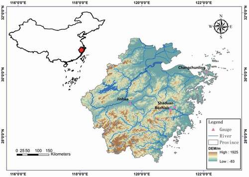
Shaduan and Bozhiao hydrological stations are located in the middle and upper regions, respectively, of Jiao River Basin; the Jiao River is in the central coastal area of Zhejiang Province between 28°22ʹ and 29°19ʹN and between 120°14ʹ and 121°55ʹE. The total area of the basin is around 6603 $k{m}^2$, and the total length of the river is close to 206 km. The upper regions of the Jiao River Basin are affected by the landforms of cut and broken hills, and the streams are distributed vertically and horizontally. The trunk and all tributaries are mountainous rivers with a steep slope and rapid flow, and the flood rises and falls suddenly. The main river channel in the lower section has a gentle slope, which is a tidal reach.

Jinhua gauge station is a control station in Qiantang River Basin. The station is located in the upper reaches of the main stream, with a basin area of 5953 $k{m}^2$, a length of 160 km, an average width of 38 km, and an average height of 27.4 m. This river is a mountain stream with a short source, rapid flow, and sudden rise (fall) characteristics. The Changchunling hydrological station is located in Zhoushan Islands, and the control area of the basin is about 3.9 $k{m}^2$. The northern island has low-lying and sparsely distributed features, which belong to the subtropical monsoon climate.

3.2 Observational data

Daily discharge data from four hydrological stations [Shaduan (SD), Bozhiao (BZA), Jinhua (JH), and Changchunling (CCL)] are used to obtain the monthly streamflow data series. Seventy percent of the available data is used for training and validation, and the rest of the data is used for testing to evaluate the models developed in this study, as shown in Table 2. This study focuses on the evaluation of model performance during the validation and testing periods.

Table 2. Data information for all gauge stations

Station name	Drainage area ($k{m}^2$)	Mean monthly streamflow ($m^3/\mathrm{s}$)	Period of record	Training	Validation	Testing
Bozhiao (BZA)	2700	40.08	1986–2018	1986–1995	1996–2007	2008–2018
Shaduan (SD)	1482	71.31	1966–2018	1966–1983	1984–2002	2003–2018
Jinhua (JH)	5990	137.53	1961–2000	1961–1973	1974–1988	1989–2000
Changchunling (CCL)	3.9	0.09	2002–2011	2002–2004	2005–2008	2009–2011

4 Results and discussion

4.1 Forecasts without baseflow and surface runoff

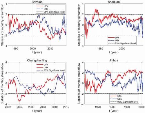
The results of the MK test are shown in Fig. 3. It is evident that the monthly streamflow at the BZA station showed no significant downward trend. It is worth mentioning that the streamflow variation is a partially random process, and the future trend has a long-term correlation with its historical change trend. In contrast, the monthly streamflow time series of the SD station shows no significant increasing trend between 1971 and 2018, but the MK test results also display a slightly downward trend during 1966–1970. The monthly streamflow of the CCL station has no definite direction of variation. According to the MK test results for the JH station, a decreasing trend appears in the streamflow time series from 1961 to 1974. However, the data shows a significant increasing trend after 1974. Additionally, the MK test results for BZA, CCL, and SD stations indicate that all of their streamflow time series can be considered stationary, while that of the JH station is determined by the non-stationary streamflow series. Table 3 lists trend analysis results for each of the 12 months at the four hydrological stations. The April streamflow at BZA and the May streamflow at JH show significant decreasing trends, and the August streamflow at SD and JH shows upward trends. Moreover, SD and JH display an increasing trend of monthly streamflow in December and March, respectively, whereas the monthly streamflow of the remaining months shows no significant trend.

Table 3. Trend analysis results using the MK test for each of the 12 months at four hydrological stations

Station	January	February	March	April	May	June	July	August	September	October	November	December
BZA	→	→	→	↓	→	→	→	→	→	→	→	→
SD	→	→	→	→	→	→	→	↑	→	→	→	↑
CCL	→	→	→	→	→	→	→	→	→	→	→	→
JH	→	→	↑	→	↓	→	→	↑	→	→	→	→

Note: →,↑, and↓ represent no trend, upward trend, and downward trend, respectively.

Figure 3. Trend analysis results using the MK test at four hydrological stations

In this section, results from six long-term streamflow forecasting models applied to predict monthly streamflow values at four hydrological stations are discussed. Each model was trained using the antecedent monthly streamflow as a predictor. Results, including NSEC and Bias% performance metrics for the testing and validation periods, are provided in Table 4. Overall, the performance metrics indicate that ANN models performed better than the statistical model. Comparing forecasting results of LSTM, GRU, BP, SVM, HW, and SARIMA models at the BZA station, it is found that the BP model had the highest values of NSEC (0.85 and 0.82) and the lowest Bias% values (−0.01 and 0.02) in the testing and validation periods, respectively. The performances in the validation period were slightly poorer than those of the testing period. This is expected because of the internal mechanism of the neural network model. Conversely, the NSEC value of the LSTM model was higher than those of the other models for the SD gauge station. It is observed that the lowest Bias% (0.28) was displayed at the CCL station when using the HW model, which demonstrates that the statistical models with long time series produce greater accuracy compared with those using shorter time series. The Bias% values (0.12) of the GRU model in the JH station for the testing and validation datasets were less than those for the other five models.

Table 4. Performance metrics of long-term streamflow forecasting models during the testing and validation periods

		Validation		Testing
Station	Model	NSEC	Bias (%)	NSEC	Bias (%)
Bozhiao	LSTM	0.81	1.17	0.80	−1.36
	GRU	0.82	1.21	0.81	3.53
	BP	0.85	−0.01	0.82	0.02
	SVM	0.42	−10.3	0.30	−15.90
	HW	0.32	−0.70	0.29	−9.66
	SARIMA	0.35	4.13	0.26	−4.30
Changchunling	LSTM	0.82	0.84	0.73	0.86
	GRU	0.78	0.69	0.70	1.36
	BP	0.80	1.06	0.74	1.32
	SVM	0.52	−14.77	0.27	−25.08
	HW	0.49	−0.02	0.31	0.28
	SARIMA	0.15	0.84	0.20	7.22
Jinhua	LSTM	0.84	0.35	0.72	−0.36
	GRU	0.81	−0.26	0.80	0.12
	BP	0.83	−0.43	0.81	0.57
	SVM	0.44	−10.68	0.39	18.31
	HW	0.43	−10.63	0.32	−14.64
	SARIMA	0.39	−1.86	0.28	−3.22
Shaduan	LSTM	0.83	0.15	0.82	0.20
	GRU	0.83	0.16	0.79	0.22
	BP	0.85	0.07	0.83	0.09
	SVM	0.32	−11.96	0.31	−16.12
	HW	0.18	−16.38	0.24	−13.61
	SARIMA	0.30	2.84	0.27	−4.84

Figure 4 shows the plots of the observed and simulated monthly streamflow values based on the six models at the four hydrological stations. Based on the plots it can be concluded that the simulation values from AI-based models are closer to the observed streamflows than those of the SVM, HW, and SARIMA models. It is noteworthy that the statistical models underestimate high monthly streamflow values. However, the LSTM, GRU, and BP models provide excellent performance when high streamflow values are considered, and they show great adaptability in predicting hydrological processes.

Figure 4. Observed and simulated values of monthly streamflows at (a) BZA station, (b) CCL station, (c) JH station, and (d) SD station based on the (e) LSTM, (f) GRU, (g) BP, (h) SVM, (i) HW, and (j) SARIMA models

Also, the prediction capabilities of the six long-term streamflow forecasting models for the annual maximum and minimum monthly values are compared and evaluated in this study. Figure 5 presents the relationship between annual peak values of observed and forecast monthly streamflow by the six models. Figure 5 shows that the forecasting skills of LSTM, GRU, and BP are good, with reasonable predictions of low and high streamflow values. However, it can be noted that the forecast performances of the SVM, HW, and SARIMA models for peak values are significantly affected by underestimations. The peak value simulation skill of the HW model is slightly higher than that of SVM and SARIMA. The results from AI-based models suggest weaker performance in estimating high flows than those for total streamflow values, which has been a problem in most of the AI-based models in hydrological forecasting (e.g. low flow, land surface temperature, and soil moisture downscaling) (Sahoo et al. 2019, Long et al. 2020, Aboward 2021). The prediction accuracy of AI-based models is greatly affected by the selection of prediction factors, and streamflow as a single predictor may not be able to capture the change process of high flows. Post-processing of the estimation from AI-based models can be used to improve the forecast in future studies (Dehghani et al. 2019, Zuo et al. 2020).

Figure 5. Comparison of the observed and simulated annual peak values of monthly streamflows at (a) BZA station, (b) CCL station, (c) JH station, and (d) SD station based on the (e) LSTM, (f) GRU, (g) BP, (h) SVM, (i) HW, and (j) SARIMA models

The plots of observed and forecast annual minimum monthly streamflow are shown in Fig. 6. The LSTM, GRU, and BP models not only can produce more reasonable minimum values with the long dataset but also can provide more accurate predictions using the short time series. As compared with forecasting peak value, the ANN models failed to predict the minimum value, and the use of a single predictor may have caused this situation. The scatter plots show an overestimation for the ANN models, and it can be speculated that this is because the baseflow is not be considered in the forecasting process. The surface runoff is greater in the wet season than in the dry season, and baseflow maintains the main streamflow during the no-rain period. The prediction of high flows is of great significance for flood control in the wet season, and forecasting of low flow plays a significant role in water demand regulation and ecology in the dry season. The most important factor in AI-based models for hydrological forecasting is the selection of predictors and their use as effective predictors to improve the forecasting accuracy of high flows and low flows. Therefore, baseflow and surface runoff are suggested for use in forecasting models in the next section.

Figure 6. Comparisons of the observed and simulated annual minimum values of monthly streamflow at (a) BZA station, (b) CCL station, (c) JH station, and (d) SD station by the (e) LSTM, (f) GRU, (g) BP, (h) SVM, (i) HW, and (j) SARIMA models

4.2 Forecasts with baseflow and surface runoff

In this section, daily baseflow and surface runoff were separated by the LH method. Based on daily data, monthly baseflow and surface runoff values are obtained. Table 5 shows the statistical summary of monthly baseflow in the CCL and JH hydrological stations, including mean, standard deviation, median, BFI (Baseflow Index)(calculated from the sum of baseflow divided by the total of streamflow) stationary condition of time series. In more detail, the baseflow dataset of the CCL station is stationary, while that of JH shows a non-stationary (upward) trend. It is apparent from the data shown in Table 5 that the BFI value of the CCL gauge station is almost double compared with those from the JH station. Here, BFI could be related to the geographical characteristics of the basins. The CCL station is located in an island basin, which means that the proportion of surface runoff is much larger than the baseflow.

Table 5. Statistical summary of monthly baseflows at stations CCL and JH

Station	Mean ($m^3/s)$	Standard deviation $(m^3/s)$	Median $(m^3/s)$	BFI	Trend
CCL	0.01	0.01	0.01	0.15	No trend
JH	40.04	31.34	31.19	0.29	Upward trend

The performance of four scenarios was assessed using the LSTM, GRU, and BP models to forecast the monthly streamflow of the CCL and JH gauge stations. AI-based models are ideally suited to select different numbers of inputs that would yield different scenarios. Furthermore, only the monthly streamflow dataset is available for the BZA and SD gauge stations, while the daily streamflow series of the CCL and JH hydrological stations are also used in different evaluations. Figure 7 shows a map of the forecasting model evaluation criteria (NSEC).As a whole, S4 (baseflow and surface runoff) performs better than other scenarios in both testing and validation periods. Higher accuracies are observed when using baseflow and surface runoff as predictors than when only streamflow is used in the prediction of monthly streamflow.

Figure 7. Forecasting model evaluation criteria (NSEC) of three long-term streamflow forecasting models (LSTM, GRU, and BP) for four scenarios at stations CCL and JH: (a–c) validation period; (d–f) testing period

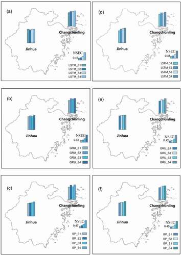
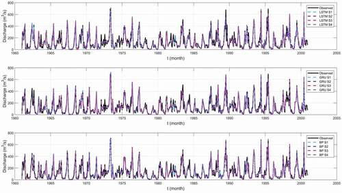
In addition, Figs 8 and 9 present the results of simulations with three models in the four scenarios. It can be seen that the hydrograph forecast by S4 is the best fitted to the observed streamflow dataset in the CCL and JH gauge stations. Notably, the highest forecast accuracy appears when using baseflow and surface runoff as two model predictors, no matter whether the streamflow series is stationary or non-stationary. Table 6 demonstrates the accuracy of the simulation by different predictor scenarios represented by NSEC and Bias%. According to Table 6, the average NSEC increased to more than 0.85, and the mean Bias% value is below 1% when using two predictors for forecasting the monthly streamflow of the CCL and JH stations. Therefore, streamflow decomposition into baseflow and surface runoff can improve the accuracy of the long-term hydrological forecast. It is apparent from the table and graphs that the BP model simulations are closer to the observed stationary streamflow series compared with the other two ANN models. In addition, the LSTM model performed better than the BP and GRU model in the non-stationary streamflow series. It is worth noting that the NSEC values of the three models were all greater than 0.7, and the Bias% was less than 10%, which demonstrates that all three models can be applied to long-term hydrological forecasting. At the JH station, the NSEC values for S1, S2, and S3 using the LSTM model are 0.72, 0.82, and 0.85, respectively. It can be concluded that the accuracy using baseflow as a predictor is higher than that from streamflow and surface runoff.

Table 6. LSTM, GRU, and BP model performance metrics for four scenarios

		LSTM				GRU				BP
Station	Scenario	Validation		Testing		Validation		Testing		Validation		Testing
		NSEC	Bias%	NSEC	Bias%	NSEC	Bias%	NSEC	Bias%	NSEC	Bias%	NSEC	Bias%
CCL	S1	0.82	0.84	0.73	1.78	0.78	0.69	0.70	1.36	0.80	1.06	0.74	1.33
	S2	0.89	0.38	0.80	1.33	0.89	0.30	0.78	1.31	0.92	0.32	0.78	0.10
	S3	0.90	0.05	0.79	0.41	0.87	3.57	0.77	1.36	0.82	−0.01	0.83	0.06
	S4	0.94	−0.01	0.85	0.86	0.90	0.55	0.84	1.12	0.95	0.20	0.85	0.22
JH	S1	0.84	0.35	0.72	−0.35	0.81	−0.26	0.80	0.12	0.83	−0.43	0.81	0.57
	S2	0.80	0.20	0.82	0.45	0.86	−0.26	0.84	1.36	0.85	−0.26	0.85	0.06
	S3	0.84	0.06	0.85	−0.13	0.84	0.07	0.84	0.21	0.95	−0.11	0.84	0.21
	S4	0.85	0.11	0.87	0.20	0.88	−0.08	0.85	0.20	0.92	−0.03	0.90	0.20

Figure 8. Observed and simulated monthly streamflow by the LSTM, GRU, and BP models for four scenarios (S1, S2, S3, and S4) at the CCL hydrological station

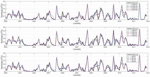
Figure 9. Observed and simulated monthly streamflow by the LSTM, GRU, and BP models for four scenarios (S1, S2, S3, and S4) at the JH hydrological station

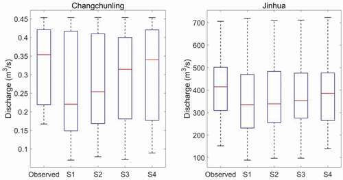
As mentioned in the previous section, in Scenario S1, the simulation of the annual peak monthly discharge of neural network models is better than that of statistical models. The observed and simulated annual peak values of monthly streamflow by four scenarios using three models in the two hydrological stations are shown in Fig. 10. It is found that the peak streamflow simulation of S4 is better than that of the other scenarios, and its median value for the annual peak streamflow series is the closest to that of observed streamflow. The upper and lower boundary values of the S4 box are similar to those of the original data box. These results suggest that S4 can provide better performance to forecast annual peak value and a comparably reasonable prediction range.

Figure 10. Comparison of the observed and simulated annual peak values of monthly streamflow at the two hydrological stations for four scenarios (S1, S2, S3, and S4) using the LSTM, GRU, and BP models

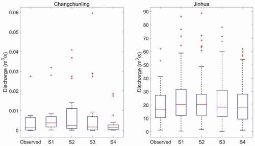
The best models thus include LSTM and BP networks at the CCL and JH stations, respectively. Therefore, the above models are used to compare the simulation performance of annual minimum streamflow in different scenarios. Figure 11 shows the box plots of observed and simulated annual minimum values for monthly discharge models from the four scenarios. According to the figure, simulations using either a single forecasting factor or two forecasting factors show overestimation. The performance of the AI-based model from S3 (baseflow as a predictor) is slightly better compared to those of the other three scenarios in the CCL hydrological station. In contrast, S4 produces reasonable forecast results using the AI-based model at the JH station. Improving the accuracy of high flows and low flows in long-term streamflow forecasting methods has always been a major area of emphasis for water resource management. When the streamflow series is selected as the forecast factor of AI-based models for extrapolation, the forecasting results of the model will be overestimated or underestimated. Based on the above results, it can be concluded that the prediction accuracy of annual maximum and minimum streamflow can be effectively improved by adding the baseflow module to the long-term hydrological forecast.

Figure 11. Comparison of the observed and simulated annual minimum values of monthly streamflow at the two hydrological stations for four scenarios (S1, S2, S3, and S4) using the LSTM, GRU, and BP models

4.3 Comparison between S1 and S4

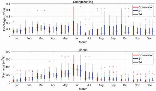
In this section, S1 and S4 present the two scenarios using a single predictor (streamflow) and two predictors (baseflow and surface runoff) in the AI-based models for monthly streamflow forecasting. The model forecasting performance of each month and the forecasting skill of the long-foreseen period have been evaluated. The box plots of simulated and observed monthly streamflow (January to December) from S1 and S4 in the CCL and JH hydrological stations are shown in Fig. 12. The results show that S4 can give better prediction performance than S1, and it could provide reliable and accurate forecasting ranges for all 12 months (January to December) at CCL and JH stations. The AI-based model using baseflow and surface runoff as predictors can forecast te more accurate values for the outliers from January to December. It can be observed that there is not much difference in the prediction skills between the two scenarios in the wet season. Also, in the dry season, the performance of S4 is much better than that of S1 using the LSTM and BP models at both stations. The inclusion of baseflow in the models could develop better prediction results for low flow, and the inclusion of surface runoff can provide better predictions of high flow.

Figure 12. Observed and simulated monthly streamflow from January to December at hydrological stations CCL and JH by the LSTM, GRU, and BP models for S1 and S4

To further verify the accuracy of the model prediction from different scenarios, we selected the streamflow series from the last year to validate the AI-based model performance and the rest of the data for training and testing. In addition, Table 7 shows the long-term streamflow forecast results based on S1 and S4 during six months’ lead time at the JH and CCL gauge stations. We can see that the overall forecasting model performance of S1 is similar to that of S4 in the first two months for both stations, and the Bias% values are less than 5%. However, for the long-foreseen period, S1 declines in performance when using the LSTM and BP models at the CCL and JH stations, respectively. At both stations, the monthly streamflow forecasting result of S4 exhibits better agreement with the observed values than does that of S1. Moreover, adding the baseflow separation process in the AI-based models to forecast long-term streamflow would extend the lead time, which can solve the problem of a short-foreseen period caused by traditional forecasting models. It is noted that the AI-based models, by adding baseflow and surface runoff as predictors, can provide good simulation results.

Table 7. Long-term streamflow forecast results of Scenarios 1 and 4 during a six-month forecasting period at the JH and CCL hydrological stations

Month	CCL LSTM model streamflow ($m^3/s)$					JH BP model streamflow ($m^3/s)$
	Observation	S1	Bias %	S4	Bias %	Observation	S1	Bias %	S4	Bias %
1	0.0122	0.0128	4.92	0.0121	0.82	41.38	39.78	−3.87	42.95	3.79
2	0.0195	0.0201	3.08	0.0186	−4.62	77.67	74.26	−4.39	75.59	−2.68
3	0.0276	0.0255	−7.61	0.0268	2.89	199.91	172.11	−13.91	213.37	6.73
4	0.0099	0.0089	−10.11	0.0107	8.08	75.96	83.32	9.69	72.63	−4.39
5	0.0019	0.0023	21.05	0.0017	−10.53	44.27	53.81	21.55	48.97	10.62
6	0.4537	0.5822	28.32	0.5137	13.22	637.81	478.55	−24.97	548.61	−13.99

CCL (Changchunling), LSTM (Long Short-Term Memory), JH (Jinhua), BP (Back-Propagation).

5 Conclusions

Investigation of the performance of long-term streamflow forecast using conventional and AI-based models is the main focus of this work. This study proposed and evaluated six monthly streamflow forecasting models (LSTM, GRU, BP, SVM, HW, and SARIMA). These models were applied to four sites in Zhejiang Province, China. In addition, the prediction accuracies of different models under the same forecast scenario were compared and analysed. Meanwhile, stationarity of streamflow time series was considered in long-term prediction, which can help in assessing the suitability of a forecasting model for stationary and non-stationary streamflow series. In addition, four scenarios were then designed for evaluating different roles of baseflow and surface runoff for long-term streamflow forecasting. The main findings of this study are summarized as follows:

1. The historical streamflow data are found to be stationary (no trend) at the BZA, SD, and CCL gauge stations, while the data for the JH station shows a statistically significant upward trend. In the model prediction based on a single prediction factor (monthly streamflow), the forecasting accuracy of the ANN models is much higher than that of the statistical model in the stationary and non-stationary streamflow series. The NSEC value for the LSTM, GRU, and BP models is more than 0.80, and the Bias% of model simulation is less than 15%, which can meet the requirements of long-term hydrological forecasts. However, for the annual minimum monthly streamflow simulation, the SVM, HW, and SARIMA models produced overestimation, and the simulation accuracy is not as high as that of the ANN models.

2. Streamflow, baseflow, and surface runoff play essential roles in long-term hydrological forecasting. The forecasting results of the ANN models with two predictor variables (baseflow and surface runoff) are found to be more reasonable than those using a single predictor, no matter whether the streamflow series is stationary or non-stationary. Moreover, the simulation accuracy of annual peak and minimum monthly streamflow was also improved.

3. Scenario S4 can give better predictions than S1, and it could provide reliable and accurate forecasting ranges for all 12 months (January to December) at the CCL and JH stations. Then, adding the baseflow separation process in the AI-based models to forecast long-term streamflow would extend the prediction period.

Based on the above results, it is proposed to add the baseflow and surface runoff as model predictors to the long-term streamflow forecast, and the ANN models also improved the performance skills of the stationary or non-stationary streamflow series. These models can be applied to other basins in the future to realize the optimal allocation and efficient utilization of water resources in the basin.

Acknowledgements

The authors thank the Major Project of Natural Science Foundation of Zhejiang [LZ20E090001], the Fundamental Research Funds for the Zhejiang Provincial Universities [2021XZZX015], and the Zhejiang Key Research and Development Plan [2021C03017] for financial support. Zhejiang Bureau of Hydrology is also greatly acknowledged for providing hydrologic data used in this study.

Disclosure statement

No potential conflict of interest was reported by the authors.

Additional information

Funding

This work was supported by the Fundamental Research Funds for the Zhejiang Provincial Universities [grant number 2021XZZX015]; Zhejiang Key Research and Development Plan [grant number 2021C03017]; and the Major Project of Natural Science Foundation of Zhejiang [grant number LZ20E090001].

References

- Aboward, A.S., 2021. Generating surface soil moisture at 30 m spatial resolution using both data fusion and machine learning toward better water resources management at the field scale. Remote Sensing of Environment, 255, 112301. doi:https://doi.org/10.1016/j.rse.2021.112301
- Ahiablame, L., et al., 2013. Estimation of annual baseflow at ungauged sites in Indiana USA. Journal of Hydrology, 476, 13–27. doi:https://doi.org/10.1016/j.jhydrol.2012.10.002
- Ajmal, M., et al., 2015. Investigation of SCS-CN and its inspired modified models for runoff estimation in South Korean watersheds. Journal of Hydro-environment Research, 9 (4), 592–603. doi:https://doi.org/10.1016/j.jher.2014.11.003
- Bhandari, S., 2019. Streamflow forecasting using singular value decomposition and support vector machine for the upper rio grande river basin. Journal of the American Water Resources Association, 55 (3), 680–699. doi:https://doi.org/10.1111/1752-1688.12733
- Block, P., 2011. Tailoring seasonal climate forecasts for hydropower operations. Hydrology and Earth System Sciences, 15 (4), 1355–1368. doi:https://doi.org/10.5194/hess-15-1355-2011
- Box, G.E.P. and Jenkins, G.M., 2010. Time series analysis: forecasting and control. Journal of Time, 31 (4), 303. doi:https://doi.org/10.1111/j.1467-9892.2009.00643.x
- Carlson, R.F., MacCormick, A.J.A., and Watts, D.G., 1970. Application of linear random models to four annual streamflow series. Water Resources Research, 6 (4), 1070–1078. doi:https://doi.org/10.1029/WR006i004p01070
- Cartwright, I., Gilfedder, B., and Hofmann, H., 2014. Contrasts between estimates of baseflow help discern multiple sources of water contributing to rivers. Hydrology and Earth System Sciences, 18 (1), 15–30. doi:https://doi.org/10.5194/hess-18-15-2014
- Chapelle, O., et al., 2002. Choosing multiple parameters for support vector machines. Machine Learning, 46 (1–3), 131–159. doi:https://doi.org/10.1023/A:1012450327387
- Chen, H. and Teegavarapu, S.V.R., 2020. Comparative analysis of four baseflow separation methods in the south Atlantic-Gulf Region of the U.S. Water, 12 (1), 120. doi:https://doi.org/10.3390/w12010120
- Cheng, L., et al., 2012. Exploring the physical controls of regional patterns of flow duration curves - part 1: insights from statistical analyses. Hydrology and Earth System Sciences, 16 (11), 4435–4446. doi:https://doi.org/10.5194/hess-16-4435-2012
- Cheng, L., Zhang, L., and Brutsaert, W., 2016. Automated selection of pure base flows from regular daily streamflow data: objective algorithm. Journal of Hydrologic Engineering, 21 (11), 06016008. doi:https://doi.org/10.1061/(ASCE)HE.1943-5584.0001427
- Cheng, M., et al., 2020a. Long lead-time daily and monthly streamflow forecasting using machine learning methods. Journal of Hydrology, 590, 125376. doi:https://doi.org/10.1016/j.jhydrol.2020.125376
- Cheng, S., et al., 2020b. Evaluation of baseflow modelling structure in monthly water balance models using 443 Australian catchments. Journal of Hydrology, 591, 125572. doi:https://doi.org/10.1016/j.jhydrol.2020.125572
- Cho, K., et al., 2014. Learning phrase representations using RNN encoder–decoder for statistical machine translation. In Proceedings of the 2014 Conference on Empirical Methods in Natural Language Processing (EMNLP), Stroudsburg, PA, USA: Association for Computational Linguistics, 1724–1734.
- Cooper, E.S., et al., 2018. Observation impact, domain length and parameter estimation in data assimilation for flood forecasting. Environmental Modelling and Software, 104, 199–214. doi:https://doi.org/10.1016/j.envsoft.2018.03.013
- Corzo, G. and Solomatine, D., 2007. Knowledge-based modularization and global optimization of artificial neural network models in hydrological forecasting. Neural Networks, 20 (4), 528–536. doi:https://doi.org/10.1016/j.neunet.2007.04.019
- Dehghani, M., Seifi, A., and Riahi-Madvar, H., 2019. Novel forecasting models for immediate-short-term to long-term influent flow prediction by combining ANFIS and grey wolf optimization. Journal of Hydrology, 576, 698–725. doi:https://doi.org/10.1016/j.jhydrol.2019.06.065
- Fashae, O.A., et al., 2019. Comparing ANN and ARIMA model in predicting the discharge of River Opeki from 2010 to 2020. River Research and Applications, 35 (2), 169–177. doi:https://doi.org/10.1002/rra.3391
- Hassan, M. and Hassan, I., 2020. Improving ANN-based streamflow estimation models for the Upper Indus Basin using satellite-derived snow cover area. Acta Geophysica, 68 (6), 1791–1801. doi:https://doi.org/10.1007/s11600-020-00491-4
- Hochreiter, S. and Schmidhuber, J., 1997. Long short-term memory. Neural Computation, 9 (8), 1735–1780. doi:https://doi.org/10.1162/neco.1997.9.8.1735
- Huang, Z.Q., et al., 2020. Differing roles of base and fast flow in ensemble seasonal streamflow forecasting: an experimental investigation. Journal of Hydrology, 591, 125272. doi:https://doi.org/10.1016/j.jhydrol.2020.125272
- Humphrey, G.B., et al., 2016. A hybrid approach to monthly streamflow forecasting: integrating hydrological model outputs into a Bayesian artificial neural network. Journal of Hydrology, 540, 623–640. doi:https://doi.org/10.1016/j.jhydrol.2016.06.026
- Kao, I.-F., et al., 2020. Exploring a long short-term memory based encoder-decoder framework for multi-step-ahead flood forecasting. Journal of Hydrology, 583, 124631. doi:https://doi.org/10.1016/j.jhydrol.2020.124631
- Kays, H.M.E., et al., 2018. A collaborative multiplicative Holt-Winters forecasting approach with dynamic fuzzy-level component. Applied Sciences, 8 (4), 530. doi:https://doi.org/10.3390/app8040530
- Kim, T., et al., 2021. Can artificial intelligence and data-driven machine learning models match or even replace process-driven hydrologic models for streamflow simulation?: a case study of four watersheds with different hydro-climatic regions across the CONUS. Journal of Hydrology, 598, 126423. doi:https://doi.org/10.1016/j.jhydrol.2021.126423
- Kratzert, F., et al., 2018. Rainfall–runoff modelling using long short-term memory (LSTM) networks. Hydrology and Earth System Sciences, 22 (11), 6005–6022. doi:https://doi.org/10.5194/hess-22-6005-2018
- Li, F., Wang, Z.-Y., and Qiu, J., 2019. Long-term streamflow forecasting using artificial neural network based on preprocessing technique. Journal of Forecasting, 38 (3), 192–206. doi:https://doi.org/10.1002/for.2564
- Long, D., et al., 2020. Generation of MODIS-like land surface temperatures under all-weather conditions based on a data fusion approach. Remote Sensing of Environment, 246, 111863. doi:https://doi.org/10.1016/j.rse.2020.111863
- Longobardi, A., et al., 2018. Regression approaches for hydrograph separation: implications for the use of discontinuous electrical conductivity data. Water, 10 (9), 1235. doi:https://doi.org/10.3390/w10091235
- Lott, D.A. and Stewart, M.T., 2016. Base flow separation: a comparison of analytical and mass balance methods. Journal of Hydrology, 535, 525–533. doi:https://doi.org/10.1016/j.jhydrol.2016.01.063
- Loveridge, M., Rahman, A., and Hill, P., 2017. Applicability of a physically based soil water model (SWMOD) in design flood estimation in eastern Australia. Hydrology Research, 48 (6), 1652–1665. doi:https://doi.org/10.2166/nh.2016.118
- Lucas, M.C., et al., 2021. Significant baseflow reduction in the Sao Francisco River Basin. Water, 12, 2. doi:https://doi.org/10.3390/w13010002
- Lv, N., et al., 2020. A long short-term memory cyclic model with mutual information for hydrology forecasting: a case study in the xixian basin. Advances in Water Resources, 141, 103622. doi:https://doi.org/10.1016/j.advwatres.2020.103622
- Lyne, V. and Hollick, M., 1979. Stochastic time-variable rainfall-runoff modelling. Proceedings of the hydrology and water resources symposium. Institute of Engineers Australia National Conference, Perth.
- Mann, H.B., 1945. Nonparametric tests against trend. Econometrica, 13 (3), 245–259. doi:https://doi.org/10.2307/1907187
- Mendoza, P.A., et al., 2017. An intercomparison of approaches for improving operational seasonal streamflow forecasts. Hydrology and Earth System Sciences, 21 (7), 3915–3935. doi:https://doi.org/10.5194/hess-21-3915-2017
- Nathan, R.J. and McMahon, T.A., 1990. Evaluation of automated techniques for base flow and recession analyses. Water Resources Research, 26 (7), 1465–1473. doi:https://doi.org/10.1029/WR026i007p01465
- Papacharalampous, G. and Tyralis, H., 2020. Hydrological time series forecasting using simple combinations: big data testing and investigations on one-year ahead river flow predictability. Journal of Hydrology, 590, 125205. doi:https://doi.org/10.1016/j.jhydrol.2020.125205
- Phan, T.T.J. and Nguyen, X.H., 2020. Combining statistical machine learning models with ARIMA for water level forecasting: the case of the Red river. Advances in Water Resources, 142, 103656. doi:https://doi.org/10.1016/j.advwatres.2020.103656
- Pumo, D., Viola, F., and Noto, L., 2016. Generation of natural runoff monthly series at ungauged sites using a regional regressive model. Water, 8 (5), 209. doi:https://doi.org/10.3390/w8050209
- Riad, S., et al., 2004. Rainfall-runoff model using an artificial neural network approach. Mathematical and Computer Modelling, 40 (7–8), 839–846. doi:https://doi.org/10.1016/j.mcm.2004.10.012
- Robertson, D.E. and Wang, Q.J., 2012. A Bayesian approach to predictor selection for seasonal streamflow forecasting. Journal of Hydrometeorology, 13 (1), 155–171. doi:https://doi.org/10.1175/JHM-D-10-05009.1
- Sahoo, B.B., et al., 2019. Long short-term memory (LSTM) recurrent neural network for low-flow hydrological time series forecasting. Acta Geophysica, 67 (5), 1471–1481. doi:https://doi.org/10.1007/s11600-019-00330-1
- Sattari, M.T., Yurekli, K., and Pal, M., 2012. Performance evaluation of artificial neural network approaches in forecasting reservoir inflow. Applied Mathematical Modelling, 36 (6), 2649–2657. doi:https://doi.org/10.1016/j.apm.2011.09.048
- Tan, Q.F., et al., 2018. An adaptive middle and long-term runoff forecast model using EEMD-ANN hybrid approach. Journal of Hydrology, 567, 767–780. doi:https://doi.org/10.1016/j.jhydrol.2018.01.015
- Tongal, H. and Booij, M.J., 2018. Simulation and forecasting of streamflows using machine learning models coupled with base flow separation. Journal of Hydrology, 564, 266–282. doi:https://doi.org/10.1016/j.jhydrol.2018.07.004
- Turan, M.E. and Yurdusev, M.A., 2014. Predicting monthly river flows by genetic fuzzy systems. Water Resources Management. 28, 4685–4697. doi:https://doi.org/10.1007/s11269-014-0767-z
- Turner, S.W.D., et al., 2017. Complex relationship between seasonal streamflow forecast skill and value in reservoir operations. Hydrology and Earth System Sciences, 21 (9), 4841–4859. doi:https://doi.org/10.5194/hess-21-4841-2017
- Vapnik, V.N., 1998. Statistical learning theory. New York: John Wiley and Sons, Inc.
- Vivekanandan, N.J.M., 2011. Prediction of annual runoff using artificial neural network and regression approaches. Mausam, 62 (1), 11–20
- Wang, Z.-Y., Qiu, J., and Li, -F.-F., 2018. Hybrid models combining EMD/EEMD and ARIMA for long-term streamflow forecasting. Water, 10 (7), 853. doi:https://doi.org/10.3390/w10070853
- Werbos, P.J., 1990. Backpropagation through time: what it does and how to do it. Proceedings of the IEEE, 78 (10), 1550–1560. doi:https://doi.org/10.1109/5.58337
- Xie, J.X., et al., 2020. Evaluation of typical methods for baseflow separation in the contiguous United States. Journal of Hydrology, 583, 124628. doi:https://doi.org/10.1016/j.jhydrol.2020.124628
- Yang, T., et al., 2017. Developing reservoir monthly inflow forecasts using artificial intelligence and climate phenomenon information. Water Resources Research, 53 (4), 2786–2812. doi:https://doi.org/10.1002/2017WR020482
- Yu, X., et al., 2020. Comparison of support vector regression and extreme gradient boosting for decomposition-based data-driven 10-day streamflow forecasting. Journal of Hydrology, 582, 124293. doi:https://doi.org/10.1016/j.jhydrol.2019.124293
- Zhang, D., et al., 2018. Modeling and simulating of reservoir operation using the artificial neural network, support vector regression, deep learning algorithm. Journal of Hydrology, 565, 720–736. doi:https://doi.org/10.1016/j.jhydrol.2018.08.050
- Zhao, T., Schepen, A., and Wang, Q.J., 2016. Ensemble forecasting of sub-seasonal to seasonal streamflow by a Bayesian joint probability modelling approach. Journal of Hydrology, 541, 839–849. doi:https://doi.org/10.1016/j.jhydrol.2016.07.040
- Zhou, J., et al., 2018. Data pre-analysis and ensemble of various artificial neural networks for monthly streamflow forecasting. Water, 10 (5), 628. doi:https://doi.org/10.3390/w10050628
- Zhu, S., et al., 2016. Streamflow estimation by support vector machine coupled with different methods of time series decomposition in the upper reaches of Yangtze River, China. Environmental Earth Sciences, 75 (6), 6. doi:https://doi.org/10.1007/s12665-016-5337-7
- Zuo, G.G., et al., 2020. Two-stage variational mode decomposition and support vector regression for streamflow forecasting. Hydrology and Earth System Sciences, 24 (11), 5491–5518. doi:https://doi.org/10.5194/hess-24-5491-2020