Understanding flood seasonality and flood regime shift in the Congo River Basin

ABSTRACT

In the sparsely investigated region of the Congo Basin (CB), flood seasonality and flood regime shift are established through relative frequency, cluster analysis, directional statistics, and non-overlapping block methods based on block maxima and peak over threshold (POT) series. Two months of significantly rich floods are observed at all gauging stations. The spatial distribution of floods presents three patterns: the north and northwest pattern, south and southeast pattern, and west/east pattern. It is observed that unimodal flood distribution is coherent in the northern and southern parts, as opposed to the bimodal flood distribution observed along the large band of the Equator from west to east of the basin. The time lag of flood indices suggests that the flood regime is not stationary. In addition, the time series show periods of high flooding, with POT frequencies and amplitudes higher during the 1960s and early 1970s than any other time period.

KEYWORDS:

• Congo Basin
• directional statistics
• mean day
• regime shift
• seasonality

Editor A. Fiori; Associate editor A. Efstratiadis

1 Introduction

Information on flood seasonality is required in many practical applications of water resources management, such as seasonal streamflow forecasting, river basin flood protection, flood-plain management, recession agriculture planning, pre-disaster planning and preparedness, and water resources infrastructure operation (Cunderlik et al. 2004a). Flood seasonality helps to delineate regions with hydrologically homogeneous characteristics (Burn 1997, Cunderlik and Burn 2002, Ouarda et al. 2006). Also, in flood frequency models, flood seasonality information assists in separating mixed-distribution flood-generated factors (Ouarda et al. 2000). In addition, the global environment is rapidly changing as a consequence of increasing impacts and pressures on the natural system. Changes in climate or the environment may alter hydrological processes at the catchment scale, with subsequent impacts on water-related risks, which may cause damages to human lives, food production systems and infrastructures.

Due to its dramatic effects on infrastructure and people, flooding is often viewed as negative; however, this is not always the case. Flooding can also provide many benefits, including recharging groundwater, increasing fish production, creating wildlife habitat, recharging wetlands, constructing floodplains, and rejuvenating soil fertility (Poff 2018, Talbot et al. 2018). In this regard, understanding flood seasonality is of paramount importance for many practical applications.

Until now, the limited availability of good-quality data has largely permitted studies on flood seasonality only in Europe and America. For example, Ouarda et al. (1993) investigated the seasonality of floods in Canada. They used directional statistics and the relative frequencies method to delineate hydrologically homogeneous regions. Collins et al. (2014) assessed flood seasonality for 22 river gauges across New England and Atlantic Canada with near-natural flood-generating conditions by computing the relative frequency of annual maximum floods across four seasonal groups. Their results indicated that the annual timing of flood-rich seasons has generally not shifted over the period of record, but 65 sites with data from 1941 to 2013 revealed increased numbers of June–October floods. Ye et al. (2017) enhanced the classification of flood seasonality in the United States, and interpreted the flood-generating mechanisms, by focusing on a circular statistical measure of timing variability and comparing it with the annual timing variability of maximum rainfall. Collins (2019) used the relative frequency of annual maximum flow to address the seasonality of floods across the northeast United States. He showed that flood occurrence is not limited to a specific season, although spring (March, April and May – MAM) is important at nearly all sites, and it was common throughout the region for a site to have more than one flood season. To identify seasonal floods, various analyses have been performed for several regions in Europe. Examples of recent studies include Engeland et al. (2018) for Norway, Mangini et al. (2018) across Europe, and Hannaford and Buys (2012) for the United Kingdom. These analyses offer insights into patterns of floods within particular catchments.

Schmocker-Fackel and Naef (2010) performed an analysis of flood regime change in Switzerland. They found large-scale patterns of change in flood regime, and the patterns observed in different European countries suggest that changes in large-scale atmospheric circulation are responsible for the flood fluctuations.

With regard to flood seasonality in the Congo Basin (CB), the literature shows heterogeneous patterns, which could be due to the fact that large part of the basin is under the influence of rainfall triggered by the Intertropical Convergence Zone (ITCZ) or the El Niño-Southern Oscillation (ENSO) episodes (Burn and Arnell 1993, Washington et al. 2013, Munzinmi et al. 2015). Hence, depending on the season in which flood occurs, one can surmise which phenomenon (ITCZ or ENSO) is likely involved in generating floods. Floods seasonality in the CB is mainly driven by rainfall and modulated by catchment processes, which also depend in part on human activities that take place in the basin. Dettinger and Diaz (2000) reveal that larger components of decadal streamflow and precipitation variation are found in rivers for much of tropical Africa. Flow data over the past 90 years on average suggest that some parts of the CB are experiencing upward or downward flow trends (Wesselink et al. 1996, Laraque et al. 1998, Runge and Nguimalet 2005). A study by Laraque et al. (2001), based on four statistical methods for detecting average discontinuity in flow records of the CB (Pettit’s test, Buishand’s U statistic, Lee and Heghinian’s Bayesian procedure and the Hubert segmentation test), detected decadal variability in the flow record of about 90 years for nine gauging stations. Despite the relevance of the study, it was unclear in the detection of flood period – i.e. whether it was a flood-rich (more frequent and bigger floods than usual in magnitude) or flood-poor period – which constitutes a major concern for river-based activities.

Analysis of hydrological trends in the CB, which is the area of interest of this research, shows a sharp rise in flood events and risks (Tshimanga et al. 2016, Hawker et al. 2020, Bola et al. 2022). Based on an analysis of natural disasters that were documented for the CB region between 1964 and 2012, Tshimanga et al. (2016) noted a clear increase in the trend of natural hazards, with floods representing 40% of all hazards compared to only 10% for droughts. This is without referring to the major floods that occurred in the basin during the last three years, with regional impacts on economic assets and human lives. In fact, the month of December 2019 saw the largest Congo River flood in 50 years, which reached a magnitude of 70 800 m³/s recorded at Kinshasa gauging station – only 500 km from the outlet into the Atlantic Ocean. This reportedly triggered a submarine turbidity current on 14–16 January 2020, which ran for over 1000 kilometres, and was still accelerating (to 8 m/s) 1150–1250 km from its source at the mouth of the Congo River, thus breaking seabed telecommunications cables that provide the internet and data transfer to much of West Africa and South Africa (Talling et al. 2022).

Flood disasters are frequently reported in the CB, with sometimes significant damage to socio-economic livelihoods and to the environment, but with limited data it is difficult to provide an adequate understanding of processes governing the dynamics of floods, and it is equally difficult to establish a clear policy towards flood management systems. In the effort to address this challenge, Hawker et al. (2020) estimated the uncertainty of using earth observation to capture flood events due to burned areas, cloud cover and vegetation in regions of the CB. Bola et al. (2022) established the usefulness of global flood model products in identifying risks to floods in data-scarce regions of the CB, but stressed the need for robust approaches to integrate understanding of the regional and local factors that drive natural hazards such as flood.

Following a review of studies conducted globally, as established in previous sections of this paper, it is demonstrated that seasonal flood analysis can help in understanding the pattern of flood regimes, which have direct implications for hydrology and water resources management applications. This is very important in sub-Saharan Africa, specifically in the CB, where there have been very few studies on flood pattern (Ficchi and Stephens 2019), although these are critically required for resilient development as stakeholders in the basin are currently engaging in major water resources investments. Thus, the focus of this study is to define flood seasonality and flood regime shift within the CB. This is achieved by identifying seasonal cycles of flood events and their pattern, and through the detection of unusual periods in the observations that are inconsistent with the reference condition of identical distributions. Ultimately, this study will contribute to an evolving framework of catchment classification in the CB (Tshimanga et al. 2022) that aims to provide a foundation for understanding organizational relationships and catchment response characteristics, as well as guidance for measurement and modelling, and estimates of impacts of environmental changes.

2 Study area

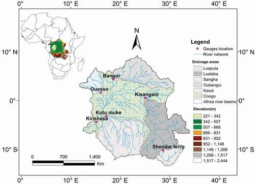
The CB is framed within 10°N, 12°E and 14°S, 34°E (corner to corner coordinates; Fig. 1), extends over 3.7 M km², and encompasses nine riparian countries: Angola, Burundi, Cameroun, Central Africa Republic (CAR), the Democratic Republic of the Congo (DRC), Republic of the Congo (RC), Rwanda, Tanzania and Zambia (Tshimanga et al. 2022). The basin is located in a transitional zone between the Sahel in the north and the Kalahari in the south, and between the Atlantic Ocean in the west and the Indian Ocean in the east. This position renders the climate particularly complex over the basin, thus making it highly vulnerable to impacts of global warming (Tshimanga and Hughes 2012, Beyene et al. 2013). The central part of the basin has low slopes, but the headwaters have steeper topography, from which flow the four main tributaries: the Oubangui River in the northeast, the Sangha River in the northwest, the Kasai River in the southwest, and the Lualaba River in the southeast. These tributaries comprise the major primary drainage units of the CB, from which the flow converges in the central basin (Cuvette Centrale) to form the main stem of the Congo River (Tshimanga and Hughes 2014).

Figure 1. Gauging stations used in the study and their corresponding drainage areas.

The hydroclimatological backgrounds that translate differences in flood seasonality in the CB are driven by rainfall associated with North/South Hemisphere movement of the ITCZ (Todd and Washington 2004). The movement of ITCZ-translated rainfall north and south of the Equator is presented in Fig. 2 (Washington et al. 2013, Alsdorf et al. 2016). The ITCZ’s proportionally greater presence in the south leads to a corresponding proportional increase in rainfall associated with the periods of ITCZ passage (Munzimi et al. 2015). Washington et al. (2013) found that rainfall associated with North/South Hemisphere movement consists of bimodal seasons with peak rainfall in the transition seasons of September to November (SON) and March to May (MAM). SON is wetter than MAM. The minimum rainfall in the June to August season (JJA) is lower than that in the December to February (DJF) dry season (Munzimi et al. 2015). Flood occurrence for the studied gauging stations coincides with rainfall peaks, which often occur around November and December in the northern and central parts of the basin, and around March to May in the southern part (Fig. 3).

Figure 2. Magnitude of north/south ITCZ translated rainfall episodes across the CB: grey indicates the location and magnitude of long-term mean monthly rainfall (JJA = 73 mm, DJF = 123 mm, SON = 160 mm, MAM = 126 mm). The green line marks the Equator (adapted from Alsdorf et al. 2016).

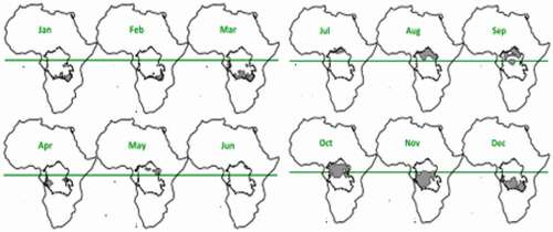
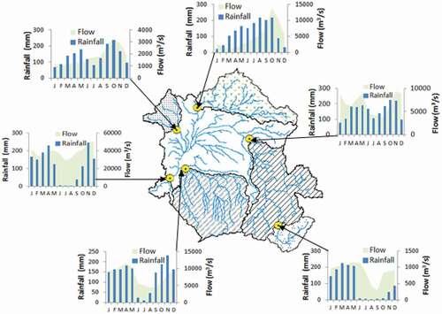
Figure 3. Congo River Rainfall and flow pattern. Blue bars indicate monthly mean rainfall (JAS = 73 mm, OND = 160 mm, JFM = 123 mm, AMJ = 146 mm). The hydrograph represents the long-term average of Congo River flow at the studied gauging stations.

Many activities in the CB are located in the floodplain near major rivers and tributaries, such that fluvial floods constitute a major issue. It is estimated that 39 million people live within 10 km of a floodplain zone of major rivers in the CB (Trigg et al. 2022). The basin is characterized by a tropical climate with high drainage density, and it is a classic example of a vast flood-prone region in Africa (Bernhofen et al. 2021). It is among the most important flood disaster hotspots in Africa (Kundzewicz et al. 2014, Bernhofen et al. 2021). Tshimanga et al. (2016) reported that in 1999, a flood wave at Kinshasa station lasted almost three days, thus approaching the scale of the two largest flood events of the century, in 1903 and 1962. It affected tens of thousands of people in both Kinshasa (DRC) and Brazzaville (Republic of Congo), and caused serious disruption of the drinking water supply systems. In 2015, a major flood affected 8480 families across the CB including in Angola, Cameroon, DRC and Tanzania, and resulted in hundreds of fatalities and tens of thousands of individuals displaced. More recently, the 2019–2020 floods affected about 170 000 people across the RC, including 30 000 Central African and Congolese refugees, and caused the destruction of 6302 ha of agricultural fields (Reliefweb 2019). Besides the negative impact of floods in the CB, there are also ecosystem services that floods can provide. Among the ecosystem services provided by flood in the CB are hydrological services related to water resources, including services related to water supply, that can be used through extraction for purposes such as agriculture and municipal water supplies, and in situ for maintaining freshwater fish production, navigation or hydropower generation (Brummett et al. 2009; Ingram 2009, Impreza-Servisi-Coordinati 2010, Warner et al. 2019). Other services include maintenance of biophysical processes and cultural services (Hart 2000), as well as biodiversity habitat. Hydrological services also include floodplain services that diminish flood damage, and transport of sediment (Teugels and Thieme 2005).

3 Data and methods

3.1 Data

Data limitations have been a challenge for many studies aiming to address issues of hydrology and water resources management in the CB. The lack of support for research in the region, as well as the large size and remoteness of the basin, can be counted among the many factors that have contributed to the paucity of data and hydrological information for the CB. In fact, two periods are critical to hydrological monitoring in the CB: the colonial and post-colonial periods. During the colonial period, quite a number of river monitoring gauges were implemented in the basin; however, these declined after the 1960s (Tshimanga et al. 2022). In this study, we have identified river gauges that have long-term daily records and that are representative of the main drainage areas of the CB, as shown in Fig. 1. These main drainage areas (sub-basin) include the Lualaba and Luapula in the southeast, the Kasai in the southwest, the Oubangui in the northeast, the Sangha in the northwest, and the Congo main stem in the central drainage basin. These are also representative of the major physiographic and hydroclimatic regions of the CB (Tshimanga et al. 2022). Daily discharge time series were obtained from various sources, including the River Navigation Authority in DRC (RVF) through a memorandum of understanding with the Congo Basin Water Resources Research Center (CRREBaC, www.crrebac.org); the Amazon Basin Water Resources Observation Service database (SO-HYBAM 2020); and the Global Runoff Data Centre (GRDC 2020). Table 1 summarizes details of the sites and their upstream basins and records. The longest time series were obtained for the Kinshasa gauging station, with over 117 years of flow record, and the shortest time series of daily discharge data came from Kasai gauging stations, covering 43 years. The drainage area upstream of this station represents about 98% of the total CB catchment.

Table 1. Characteristics of stations used in the study.

Station	River	Water year	Watershed area (km^2)	Period of record	Series length (years)	Missing data (%)	Data source
Bangui	Oubangui	April – March	490 460	1936 − 2018	83	-	SO-HYBAM
Ouesso	Sangha	March– February	158 261	1947 − 2017	71	1	SO-HYBAM
Luapula	Luapula	November–October	162 556	1955 − 2004	50	-	GRDC
Kutu muke	Kasai	September–August	747 816	1949 − 1991	43	5	GRDC
Kinshasa	Congo	August–July	1 363 156	1903 − 2019	117	-	RVF
Kisangani	Lualaba	September–August	800 836	1950 − 2009	60	2	GRDC

SO-HYBAM: Amazon Basin Water Resources Observation Services; GRDC: Global Runoff Data Centre;

RVF: Régie des Voies Fluviales.

Data homogeneity analysis and detection of outliers were performed. Gaps in the data of up to three months were marked as “missing values.” Missing data were filled using the Nonlinear Iterative Partial Least Squares (NIPALS) algorithm (Wold 1975) within the XLSTAT software (Addinsoft 2021). The NIPALS algorithm is applied on the dataset and the obtained principal components analysis (PCA) model is used to predict the missing values.

3.2 Method

3.2.1 Flow indices

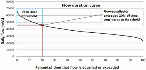
Two approaches are available for analysing flood series: (i) block maxima and (ii) peak-over-threshold (POT) approaches. Using an annual maximum series, one considers the largest event each year selected from the daily flow data (Kundzewicz et al. 2014), although in flood-rich years this might include only the largest of several large flows. Conversely, in flood-poor years a small observed flow will be selected using this method that may not necessarily be characterized as a flood at all. One way of representing high river flows in a record, regardless of when they occur, is to use a POT approach (Svensson et al. 2005). The main advantage of this latter method is that it captures all events more efficiently than annual maximum sampling does (Bačová-Mitková and Onderka 2010). In particular, the use of a POT series allows researchers to estimate the trend in the frequency of floods rather than just their magnitude, by calculating the number of POTs that occur each year and investigating the tendency in the series (Solari et al. 2017). However, the drawback of the POT method for large river systems is that multiple peaks in a year may not be independent events. In order to provide independence of the POT time series, we apply Bayliss’s criteria (Bayliss and Jones 1999) according to which the peaks in a POT series can be considered if they are separated by a particular time interval and the minimum discharge between the two peaks is less than 2/3 of the peak height recorded during the first wave. For each studied gauging station, the threshold was set based on the Q20^th (80^th percentile) value of the gauging station’s flow duration curve (Fig. 4), such that a minimum of two POT events can be selected per year.

Figure 4. Selection of peak over threshold series using daily flow based on the Q20^th value of gauging stations’ flow duration curve.

In order to ensure independence of the different flood events in large river systems of the CB, we tested different time spans of 20, 30 and 40 days between two peaks. Svensson et al. (2006) used timing that depended on catchment size: 5 days for catchments <45 000 km², 10 days for catchments between 45 000 and 100 000 km², and 20 days for catchments >100 000 km². The separation time intervals proposed by Svensson et al. (2006) allow for flow to recede appreciably between peaks. In our study, all watersheds are bigger than 45 000 km². To ensure the independence of POT events for the studied gauging stations, the time between two peak flows was set to 20 days based on the study of Olivery and Boulègue (1995) related to the recession time of peak flow over 10 catchments of the CB. Flood seasons were first identified subjectively by visually assessing the temporal distribution of flood occurrences at the site of interest. This approach is subjective and a product of sampling variability (Black and Werritty 1997, Lecce 2000). To overcome this issue, two methods were developed, one based on the distribution of monthly relative frequencies of flood occurrence (Cunderlik et al. 2004b) and the other based on directional statistics (Mardia 1975).

To obtain a comprehensive understanding of flood season and variability in the CB, we use the relative frequency method to describe the significance of floods on a monthly scale and determine the mode of flood in the studied gauging stations. The directional statistics method was used to determine the dispersion (variability) of the individual dates of flood occurrence around the mean date as well as the pattern of flood frequency on a daily basis. Thus, detailed information on flooding can be obtained from daily flood occurrence grouped into months, while the measure of central and dispersion tendency of daily flood at each gauging station must be considered as an observation on the circumference of a circle of unit radius.

3.2.2 Relative frequency method

Seasonality of flood occurrence can be tested by comparing the sampling variability of flood occurrence observed in a given record with the theoretical sampling variability of non-seasonal flood occurrences. A model of non-seasonal flood occurrence (floods with no seasonal preference) can be expressed by means of the circular uniform distribution as:

(1) $f\left(x\right)=P\left[X=x\right]=\frac{1}{{360}^0};0^0\le x<{360}^0$(1)

where x is the day of flood occurrence in degrees (by converting the 365 or 366 days of the year into 360 degrees), and $f\left(x\right)$ is the probability density function.

Seasonal analysis using the circular uniform distribution does not provide any information on the temporal occurrence of flood-rich seasons (seasons of high probability of flood occurrence), or information on the significance of flood-poor seasons (seasons of low probability of flood occurrence). To address the uncertainty resulting from the sampling variability of flood occurrences, a measure must be defined to estimate the probability of whether a given season is significant or nonsignificant. Therefore, Cunderlik et al. (2004b) suggested using a bootstrap resampling procedure to obtain a clearer picture about the sampling variability and the uncertainty associated with the estimates of flood frequency. The idea is to generate N_Bst bootstrap samples from the available record and assess the significance of flood seasons, using the approximated confidence intervals introduced by Cunderlik et al. (2004b):

(2) $P_U=\frac{N+11.491}{0.048N^{-1.131}}$(2)

(3) $P_L=\frac{N-27.832}{0.119N^{-0.964}}$(3)

where P_U and P_L are the upper and lower confidence intervals, respectively, and N = is the length of observations.

In order to classify the seasons of flood occurrence objectively, Cunderlik et al. (2004b) defined “significant flood-rich months” comprising months with relative frequencies exceeding the upper confidence interval P_U for the uniform distribution. The category of “flood-rich months” will then include months that do not exceed the upper one-sided confidence interval (P_U) but do exceed the mean value. In a similar approach, months with relative frequencies below the lower one-sided confidence interval (P_L) can be classified as “significant flood-poor months,” and those inside the confidence intervals as “flood-poor months.” Applications of the relative frequency method can be found in Ouarda et al. (2006), Liu et al. (2010), Chen et al. (2013) and Collins (2019).

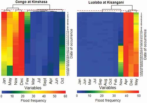
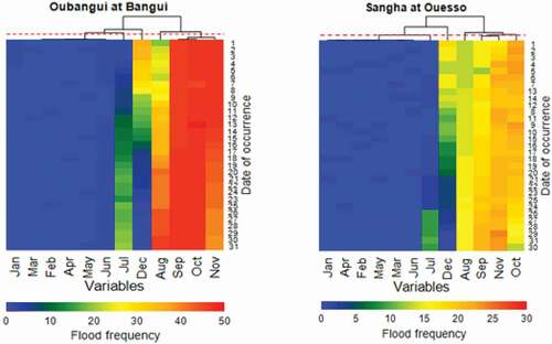
Following the study by Creese et al. (2019), flood-rich months at gauging stations were classified within CB’s wet seasons of March–May (MAM) and September–November (SON). Sites with flood‐rich months occurring in March, April and May were classified as having a MAM flood season. Sites with flood‐rich months in September, October and November were classified as having a SON flood season. The criterion for multimodal seasonality was that flood-rich months must be separated at least by one or more non-significant flood-poor months (Hall and Bloschl 2018). A unimodal flood seasonality distribution is identified if all flood-dominated months occur consecutively (Hall and Bloschl 2018). Thus, all gauges were classified as having either unimodal or multimodal flood seasons. Therefore, it is of interest to identify gauging stations with similar flood distribution characteristics (i.e. same months of flooding). In order to identify stations with similar months of flooding, each individual gauging station was further classified by cluster analysis (Wilkinson and Friendly 2009), based on the relative daily flood frequency of each month. For each gauging station, cluster analysis identifies cluster memberships of months in which floods occurred often and months in which floods happen seldom or never (Hall and Blöschl 2018). Thus, we qualitatively assessed gauging stations with relatively similar seasonal flood occurrence (i.e. months of flooding) and assigned them a particular type of flood season or mode. The aim of the analysis is to determine a basin with a single mechanism for flood generation that will have a unimodal distribution, while a basin with two mechanisms, for example MAM floods from rainfall and SON floods, may have a bimodal distribution.

The clustering method used was the unweighted pair-group method, which defines the distance between groups as the average distance between each of the members (Li Yujian and Xu Liye 2010). The clustering objects were months (vertical axis). Coherent patterns (blue to red with intermediate colours) of colour are generated through hierarchical clustering on horizontal axes, to associate the date with flood frequency in a given month.

3.2.3 Directional statistics method

Seasonality analysis of POT floods can also be accomplished using directional statistics (Mardia 1975) based on the occurrence time of hydrological extreme events within a year. Burn (1997) and Cunderlik et al. (2004b) introduced indices that reflect the mean date and variability of occurrence of extreme events. Their method implies that the individual dates of flood occurrence can be defined as an angular value (in radians) by converting the Julian day of flood occurrence (D_i) in year i (X) to an angular value (θ_i) as:

(4) ${\theta }_i=D_i\frac{2\pi }{X}$(4)

where:

• θ_i is the angular value representing the date of flood event _i;

• D_i is the flood occurrence Julian date. D_i can take values from 0 to 365, or 0 to 366 for a leap year; and

• X is the number of days in the year (X = 365, or 366 for a leap year).

For a sample of n flood events, this angular value can represent the hydrological regime of the catchment (Burn 1997).

A measure of the flood occurrence date can also be determined as a mean date. The mean date at a gauging station is represented by the mean direction $\overline{\theta i}$, defined by:

(5) ${\bar{\theta }}_i=arctg\left(\frac{\bar{y}}{\bar{x}}\right),\bar{x}\ne 0$(5)

where:

(6) $\bar{x}=\frac{1}{n}\sum _{i=1}^{n}cos{\bar{\theta }}_i$(6)

(7) $\bar{y}=\frac{1}{n}\sum _{i=1}^{n}sin{\bar{\theta }}_i$(7)

where $\bar{X}$ and $\bar{y}$ represent the x and y coordinates of the mean flood date and lie within, or on, the unit circle.

The variability of the mean date of flood occurrence can be characterized by the dimensionless parameter r, defined as:

(8) $r=\sqrt{{\bar{y}}^2+{\bar{x}}^2},0\le r\le 1$(8)

The value of r provides a measure of the spread of the date. A value close to 1 indicates a small variability in the timing of flood events, and hence stronger seasonality. That is, flood events are more likely to happen in a particular window of time every year in catchments with large r values. For catchments with small values of r, the occurrence of flood events is scattered across the year, so that the mean date is less representative of the occurrence date of flood events. The angular values (θi, ${\bar{\theta }}_{\mathrm{i}},$ and r) of flood occurrence are plotted by location on the circumference of a circle, with the start of year shown as the most easterly point and the seasons proceeding in a counter-clockwise sense (Fisher 1993). The directional flood seasonality approach is used by Black et al. (1997), Burn (1997), Bayliss and Jones (1999), Cunderlik and Burn (2002); Cunderlik et al. (2004b), Chen et al. (2013) and Collins (2018, 2019).

3.2.4 Frequency shift

Laraque et al. (2001) detected an average discontinuity in flow records of the CB, with potential impacts on flood frequency. To verify changes in flood frequencies, we divided flood frequency data into two time periods of the same length, according to the shift of hydrological regime in the CB reported by Laraque et al. (1998) and Wesselink et al. (1996). The year 1970 was chosen as the cut-off change year as it represents the point of hydrological regime shift in the CB. An analysis of variance (ANOVA) was conducted to detect statistically significant changes from the mean frequency of flood between two time periods. Levene’s test (Levene 1960) was applied to the two time periods of the flood frequency time series to verify equality (or not) of variance. Watersheds with a shift in flood frequencies are considered to have experienced major changes either in variance or in mean flood frequency.

3.2.5 Annual maxima and POT shift

When assessing possible flood-rich and flood-poor periods, short-term hydroclimatic instability must be distinguished from longer-term climatic trends (Hall et al. 2014). The initial point of any instability recognition in observed time series is to hypothesize about the type of changes (Hall and Bloschl 2018). These include step-changes in the mean, gradual changes in the mean or changes in the variability of the series (Hall et al. 2014). This study is concerned with step-changes in the mean of annual maximum time series, based on the study by Dettinger and Diaz (2000), which highlights decadal flood variation of much tropical Africa rivers. These changes are considered flood rich (periods with more frequent and larger floods than the mean in magnitude) or flood poor (periods with less frequent and smaller floods than the mean in magnitude). Based on the above, the null hypothesis states that the mean annual maximum flow of different decades does not differ within each gauging station. In formulating the hypothesis, the Statistical Package Statistica v. 7 (Stat. Soft. Inc 2004) was used to measure the dispersion of annual maximum means around the mean of annual maximum time series, as the standard error of the mean (mean ± SE), and we indicate the degree of certainty as the confidence interval (mean ± 1.96 SE). The significance level was set at .05. Gauging stations with a shift in flood regime are considered to have experienced major changes in decadal mean of annual maximum flow from the mean of the time series.

Following the study by Dettinger and Diaz (2000) on decadal flood variation in many tropical rivers, we also investigated how the POT frequencies of different decades are spread out from the mean of the time series for each gauging station. Knowing that ordinary variance estimators perform poorly in the presence of the shifts (Axt and Fried 2020), we investigated an approach based on non-overlapping blocks (Axt and Fried 2020) to estimate the variance of POT frequency from the mean of the time series. Different decades of POT frequency represent non-overlapping blocks. The blocks-estimator (${\sigma }^2$) of the variance is defined as:

(9) ${\sigma }^2=\frac{1}{m}\sum _{j=1}^m{S}_j^2$(9)

where:

(10) $S_j^2=\frac{1}{n-1}\sum _{t=1}^n{\left(Y_{j,t}-\overline{Y_j}\right)}^2$(10)

(11) ${\bar{Y}}_j=\frac{1}{n}\sum _{t=1}^n{Y}_{j,t}$(11)

where:

$Y_{j,1},\dots Y_{j,n}$ are the observations in the j^th block,

$S^2$ is the variance,

${\sigma }^2$ is the block estimator of variance under decade shift from the mean,

$m\mathrm{i}\mathrm{n}\mathrm{d}\mathrm{i}\mathrm{c}\mathrm{a}\mathrm{t}\mathrm{e}\mathrm{t}\mathrm{h}\mathrm{e}$ non-overlapping blocks,

$n$ denotes the number of observations, and

$\bar{Y}\mathrm{i}\mathrm{s}\mathrm{t}\mathrm{h}\mathrm{e}$ mean value of all observations.

Gauging stations with a shift in flood regime are considered to have experienced major changes in variance of different decades of POT from the mean of the time series.

4 Results

4.1 Flood seasonality

4.1.1 Temporal seasonality

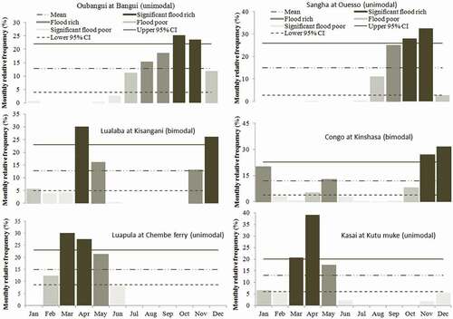
The temporal characteristics of floods were determined at each gauging station. At the monthly time scale, each of the six streamflow gauging stations presents significant flood-rich months and flood-poor months, as shown in Fig. 5. Considering the alternating occurrence of flood-rich and flood-poor months, it is clear that all of the gauging stations have two significant flood-rich months. There is an interesting dissimilarity in the flood system within the basin. The flood distribution in the Oubangui and Ouesso, which have July–December floods, contrasts with the flood systems of the Kasai and Luapula, which experience their floods from January to May. For the Lualaba and Congo, two periods of flood were found in each station. These two periods were October–January or April–May floods. Overall, the temporal distribution of floods indicates two main flood seasons: a January–May flood season and a July–December flood season. Therefore, the month of June has been identified as the month in which floods happen seldom or never over the CB. A consideration of relative frequency of flooding shows that July–December is the season with the largest amount of flooding.

Figure 5. Flood season at a monthly time step for the studied gauging stations within the CB (CI = confidence interval).

4.1.2 Spatial seasonality

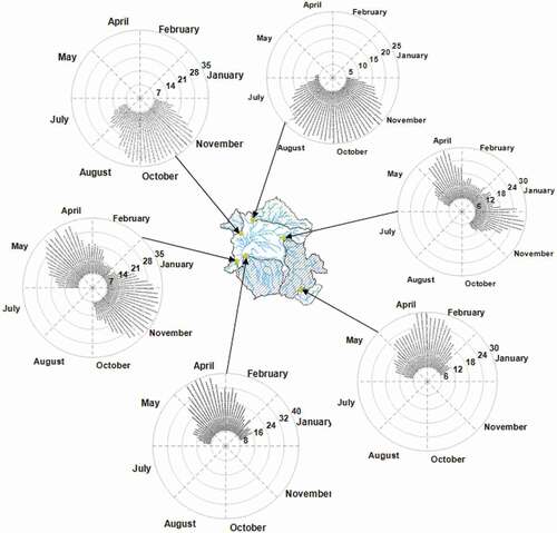
A descriptive analysis of relative flood frequency revealed a spatial pattern that can be observed in Fig. 6. Spatial coherence of flood distribution is observed between stations. Stations located in the north and northwest of the basin exhibit predominantly July–December floods. In the south, January–May floods dominate the spatial pattern. Farther west and east, floods occur in two periods, either October–January or April–May. Figure 6 shows that the spatial pattern exhibits three of flood system sequences: the south and southeast flood system, the north and northwest flood system, and the west–east system which represents the transitional pattern between the north and the south. In the west and east as well as in the central part of the basin, the flood waves of contributing catchments of the north or south are not synchronized.

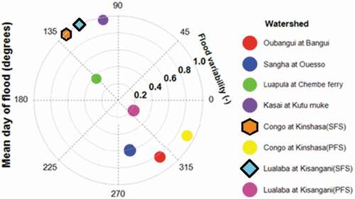
Figure 6. Flood of studied gauging stations demonstrated in radians indicating the flood distribution for a specific location; values are expressed in terms of relative frequency (%).

4.1.3 Seasonal characteristics

4.1.3.1 Seasonal similarity between stations

Cluster analysis was conducted to group months in which floods occur often and months in which floods happen seldom or never, and to determine similar months of flooding that emerge between stations. The cluster analysis shows a seasonal similarity (similar months of flood) between gauging stations (Fig. 7), details of which can be found in the Appendix (Figs A1–A3). Based on the similar months of flood that emerge, stations were grouped into four seasonal distributions (Table 2): unimodal type I, unimodal type II, bimodal type I and bimodal type II. The unimodal type I distribution encompasses Bangui and Ouesso gauging stations, where July–December floods are similar and coincide with the JJA and SON rainy season. Kasai and Luapula gauging stations have similar months of flood (January to May) and represent the unimodal type II flood distribution, characterized by a DJF and MAM rainy season. The bimodal type I distribution encompasses Congo at Kinshasa, where SON, DJF and MAM rainy seasons are involved in flood generation, with primary flood months from October to January and April–May as secondary. Lualaba at Kisangani presents a bimodal type II distribution, with November and December as the primary flood months and April to May as secondary. Flood generation in Lualaba station is linked to SON and MAM rainy seasons.

Table 2. Patterns of flood seasonality at the studied gauging stations.

Station	Months												Mode/season	Type
	January	February	March	April	May	June	July	August	September	October	November	December
													Unimodal	I
Bangui													JJA-SON
Ouesso													JJA-SON
													Unimodal	II
Shembe ferry													DJF-MAM
Kutu Muke													DJF-MAM
													Bimodal	I
Kinshasa													SON-DJF
													MAM
													Bimodal	II
Kisangani													SON
													MAM

JJA: June, July, August; SON: September, October, November; DJF: December, January, February; MAM: March, April, May.

Figure 7. Seasonal similarity between Bangui and Ouesso. The red dashed line indicates the cut in the tree clustering months in which floods occurred often and months in which floods happen seldom or never. Vertical axes display months with daily frequency within the concerned cell, coloured on the horizontal axis to associate the date of occurrence with flood frequency. Flood frequency values are expressed in terms of relative frequency (%).

4.1.3.2 Seasonal mean day and variability

By means of directional statistics, an analysis of flood mean date and variability was performed. Flood seasonality measures (mean day and variability) are described in Fig. 8. The directional mean is about 306° (2 November) for the Oubangui watershed at Bangui, 286° (12 October) for the Sanghsa at Ouesso, 137° (17 May) for the Luapula at Chembe ferry, and 106° (16 April) for the Kasai at Kutu muke. The Congo at Kinshasa, with its two flood seasons, displays a secondary directional mean of about 126° (5 May) and a primary directional mean of about 333° (29 November). The Lualaba watershed at Kisangani has two flood seasons, with a primary directional mean of about 327° (23 November) and a secondary directional mean of about 116° (26 April). Based on the above results, the major part of the basin experiences the mean day flood around November, followed by April and May. It can be seen from Fig. 8 that for the secondary flood season of Kinshasa and Lualaba as well as at Luapula and Kasai gauging stations, their mean day of floods is centred between 106° (16 April) and 137° (17 May). This suggests that in this period of 30 days CB can experience four flood events, depending on the mean day of the abovementioned gauing stations. Conversely, for the primary flood season of Kinshasa and Lualaba, as well as Sangha and Oubangui tributaries, floods are centred from 286° (12 October) to 337° (03 December). This shows that within a period of 60 days, four other flood events may occur in the CB. Specifically, the late occurrence of flood at Kinshasa gauge might be due to its location downstream of other tributaries, meaning it will exhibit an integration of their flood peaks at different times of the year. For the studied gauging stations, the variability index (r) ranged from 0.2 to 1 (Fig. 8). Sangha, Luapula and Lualaba’s primary flood season presents a weak flood seasonality (low variability index), meaning that flood events are scattered across the year, such that the mean date is less representative of flood event occurrence. Conversely, Lualaba’s secondary flood season and Kinshasa and Oubangui as well as Kasai present high flood variability index (r) values. Thus, flood events are more likely to happen at the observed mean date every year at these gauging stations.

Figure 8. Flood timing and variability expressed by the radius value (PFS = primary flood season, SFS = secondary flood season). A variability measure close to 0, i.e. in the centre of the polar plot, indicates large heterogeneity in flood timing. A variability measure close to 1 indicates that flood events tend to occur around the same day of the hydrological year.

4.2 Flood regime shift

Three flood indicators were analysed. These comprise annual maximum streamflow, absolute flood frequency and POT series. Annual maximum streamflow is the most common indicator in flood variability studies. POT series are used since they are considered to include more information and thus to better reveal the temporal pattern of flood occurrence (Svensson et al. 2006). The absolute number of flood frequencies offers the possibility to analyse changes in the number of floods occurring each period. Changes in this study refer to step-changes (regime shift) of flood indicators at a particular station.

4.2.1 Frequency shift

Frequency shift analysis requires long-term time series data, but we included the short-term time series data for other gauging stations for information purposes only. In terms of seasonal frequency before and after 1970s, some catchments exhibited shifts whilst others did not (Fig. 9). A decrease in flood frequency has been observed in the south and southeast of the CB including the Kasai and Luapula watersheds. In contrast, the Congo at Kinshasa shows a statistically significant increase in flood frequency. The northern part of the CB, which includes the Oubangui and Sangha, as well as the Lualaba in the southeast do not display significant changes in seasonal flood frequency. Overall, before the 1970s the total number of flood events was low. The post-1970s period seems to have a higher flood frequency in our records. Levene’s test allowed us to compare the mean and variance of two blocks of the flood frequency time series and find out which watersheds experienced a shift (or not) in seasonal flood frequency. These results are presented in Table 3.

Table 3. Results of Levene’s test (5% significance level (SL)) and statistics for flood frequencies.

Station	River	Levene’s test		Mean		Variance
		test value	p value	≤1970	>1970	≤1970	>1970
Bangui	Oubangui	0.727	.473	501	492	221 429	345 235
Ouesso	Sangha	1.105	.551	119	139	53 212	61 226
Luapula	Luapula	12.106	.002	127	40	11 642	829
Kutu muke	Kasai	4.279	.014	148	42	20 108	3124
Kinshasa	Congo	7.310	.004	302	1121	312 064	2 231 420
Kisangani	Lualaba	0.208	.502	278	294	3214	4988

Figure 9. Flood frequency shift demonstrated by histogram comparing flood frequency before and after the 1970s (red ≤ 1970; blue >1970).

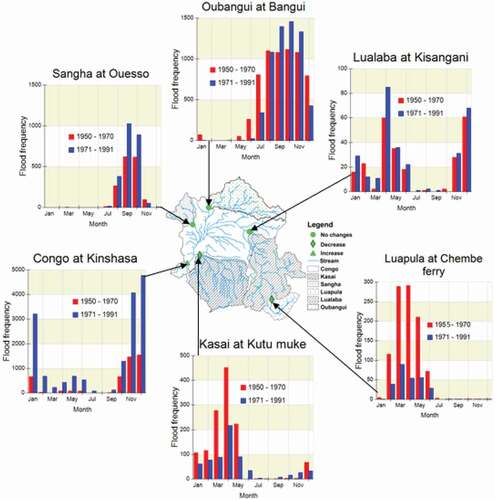
The comparison between pre- and post-1970s provided information regarding seasonal change in flood frequencies, but the decadal scale of flood dynamics as advocated by Dettinger and Diaz (2000) is provided using two flood indicators (mean annual maximum and POT).

4.2.2 Mean annual maxima shift

Flood-rich and flood-poor periods are presented according to the flood time series length of each gauging station. The dispersion of decadal mean annual maxima flow from the mean of the time series at each gauging station was observed (Fig. 10). Kinshasa gauging station recorded three decades (1951–1962, 1963–1974 and 1999–2010) of high flood magnitude corresponding to a flood-rich period, compared to four decades (1903–1914, 1928–1938, 1939–1950 and 1987–1998) of low flood magnitude, considered flood-poor periods. Indeed, Kinshasa has experienced two decades of moderate floods. Over about 58 years of flood record, the periods 1964–1974 and 1975–1985 exhibit high flood magnitude at the Kisangani gauging station compare to three decades of flood-poor period. For 42 years of observation, Kasai station exhibits larger floods over two decades (1950–1960 and 1961–1971), with one decade of low flood and one of moderate flood. The annual maximum floods at Chembe ferry were particularly high for three consecutive decades (1955–1964, 1965–1974 and 1975–1984), after which there was a decrease in flood magnitudes. About three decades (1935–1946, 1947–1958 and 1950–1970) of large floods have been recorded at Bangui, with the flood-poor period taking over just after the flood-rich period. Compared with all the stations that were analysed, Ouesso tends to show relative stability in the medium flood magnitudes over four decades, compared to one decade of high flood magnitude and one decade of low flood magnitude. An analysis of flood chronology indicates that stations were overall flood rich and flood poor with fewer moderate floods. The variability exhibits a sawtooth pattern in Kinshasa, Kasai, Kisangani and Ouesso stations, while in Bangui and Luapula there is a tendency of decreasing flood magnitude. At almost all gauging stations, the periods with higher floods than the mean in magnitude (rich periods) were identified in the 1960s and early 1970s, while the periods of poor flooding vary according to each gauging station.

Figure 10. Decadal mean annual flow maxima for specific gauging stations. For each box plot, the solid rectangle displays the mean ± standard error, dotted lines display the 95% confidence interval (mean ± 1.96 × standard error), the dashed line is the mean of the time series and the circle is the decadal mean. Whiskers of the box plot above the mean line display the flood-rich period and those below the mean line display the flood-poor period.

4.2.3 POT shift

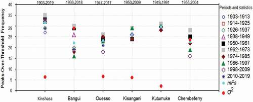
Figure 11 shows how POT frequencies at the decadal time step spread out from the mean of the time series for each gauging station. Bangui and Chembe ferry show statistically significant changes from the mean, as shown by the higher values of variance. Kinshasa, Ouesso, Kisangani and Kutu muke do not display significant changes in POT frequency and tend to show relative stability in POT frequency over decades. At all gauging stations, the decade 1962–1973 is considered a period with higher POT frequency (flood-rich period) recorded in the CB. Low POT frequencies are typical of the end of the 20th century, observed in almost all stations.

Figure 11. Decadal shift of peaks over threshold (POT) frequency from the mean of the time series for specific gauging stations. Variability reflects the time series length available at each gauging station; the values on top display the time series length of each gauging station. Different symbols correspond to different decades of POT frequency. Abbreviations: mFs: peak over threshold mean frequency of the time series; ${\sigma }^2:$ variance from the mean of the time series.

5 Discussion

The study of flow regime changes in the CB has attracted interest in the scientific literature (Wesselink et al. 1996, Laraque et al. 1998). However, the question of flood season and flood regime has not been studied. We propose three indicators (block maxima, POT and absolute frequency) to understand flood seasonality and flood regime shift.

5.1 Flood seasonality

The spatiotemporal seasonality of floods was determined at each gauging station and floods are found to occur at all times of the year, apart from the month of June when no floods are recorded. In the CB, April–May and October–December are important periods for flooding. The distribution of floods can be put into perspective by considering the hydrometeorological features of the regions and especially the south–north movement of the rain belt. For the Kasai in the South, the Chembe ferry in the southeast and the Lualaba with its secondary flood season in the east, as well as Kinshasa’s secondary flood season, MAM rainfall months tends to play an important role in flood generation. SON rainfall months play an important role in flood generation for the Sangha and Oubangui as well as for the primary flood season at Kinshasa and Kisangani. These results are consistent with Mertz et al. (2018), highlighting that catchment location and event precipitation play important roles in spatiotemporal flood responses.

The observed spatial pattern can be put into the perspective of the local seasonal cycle of precipitation, the local seasonal cycle of evaporation demand, travel times of water from runoff source areas through surface and subsurface reservoirs and channels to the streamgauge, and human management. It can be observed that the geographical location of a watershed and hence the climate of the region seems to be the relevant factor in shaping spatial coherence or heterogeneity in flood pattern. This is interesting because the proximity of regions tends to favour spatial coherence. Further, the degree of spatial coherence of flood pattern should vary between regions whose flood generation is governed by different processes (Mertz et al. 2018). Processes such as the twice-yearly passing of ITCZ in the North/South of the Equator (Munzimi et al. 2015) have led to two large regions with identical flood patterns: Oubangui and Sangha in the North, and Kasai and Shembe ferry in the South. The coherence pattern of flood in the North and South of Equator is due to the large-scale circulation of ITCZ. Large atmospheric circulation has led to spatial coherence of the flood pattern compared to regions characterized by very frequent atmospheric variability (Kiem et al. 2003, Steirou et al. 2017). The third region with a homogeneous flood pattern is observed in the large band of the Equator from west to east. This region is characterized by a bimodal flood season linked to bimodal precipitation enhanced by the atmospheric convective circulation observed in Equator region (Pokam et al. 2014). Flood seasonality of the CB varies from region to region and is influenced mostly by large atmospheric circulation and the geographical location. According to the rainfall amount triggered by large atmospheric circulation, the CB can be divided into three large regions withs homogeneous flood pattern: Oubangui–Sangha region, Kasai–Shembe ferry region and the large band of the Equator. These broad spatio-temporal patterns linked to geographical location and large atmospheric circulations are consistent with previous findings (Dettinger and Diaz 2000, Hall and Blöschl 2018).

The combination of a quantitative approach using cluster analysis of daily relative flood frequencies with a qualitative assessment of the temporal distribution of floods demonstrated similar and dissimilar patterns of the analysed gauging stations. Similarity between months in which floods occurred often and months in which floods happen seldom or never led us to aggregate gauging stations into regions of similar climatic conditions with a particular flood distribution. There is a tendency for floods to occur at around the same time in different areas of the basin. An appreciation of similarity between gauging stations and the climatic conditions that encourage them would also enable an objective assessment of the distribution of floods in recent years in relation to longer term spatial patterns. The unimodal and bimodal distributions in the CB are driven by the seasonal distribution of rainfall, and the topography and physiographical characteristics of the contributing catchments. The particularity of the bimodal flood season is that the flood waves of contributing catchments are not synchronous when they arrive in the main stem. For instance, the transfer times of water masses to Brazzaville/Kinshasa have been defined by Olivry and Boulègue (1995) as follows: one month for Congo and Upper Oubangui, two months for Lualaba and 15 days for Sangha, Cuvette Centrale and Kasai. Therefore, the Congo and Lualaba watersheds provide an example of flood patterns reflecting the complex interaction between events with varying contributions from northern and southern tributary catchments.

Using directional statistics, two measures (mean date and variability index) of flood seasonality were computed for each station. Gauging stations had different mean dates and variability indices. Given their distinct local interactions, the flood mean date and variability index differ from one catchment to another. This underlines the major importance of geographical location and physiographic characteristics of the river basin on shaping flood responses (Laraque et al. 2001). It therefore follows that the mean date and variability index of floods are also affected by drainage basin conditions, such as pre-existing water levels in rivers, the soil status (permeability, soil moisture content and its vertical distribution) and the rate of urbanization (Hölscher et al. 1997, Minasny and Hartemink 2011). The relationship between rainfall and drainage basin conditions is significant in modulating flood regimes (Nicholson 2000, Todd and Washington 2004, Wohl et al. 2012, Bischiniotis et al. 2018, Ficchì and Stephens 2019). Bischiniotis et al. (2018) also assert that precipitation is connected with most reported floods (72%), and more than half of flood events exhibited wet antecedent conditions during the six preceding months. Flood seasonality of the CB is related to precipitation triggered by large atmospheric circulation, and drainage basin location and conditions.

5.2 Flood regime shift

To date, there is evidence of flood frequency shifts in the CB. This study finds that three patterns of change (increasing, decreasing and no change) characterize the CB’s flood frequencies. It is believed that precipitation dynamics can be the driver of this change, associated with climate variability (Beyene et al. 2013, Hirabayashi et al. 2013, Creese et al. 2019). A study by Todd and Washington (2004) connected the changes in the CB’s discharge with the North Atlantic Oscillation (NAO) and suggest that changes in precipitation have impacted the flow regime which in turn can affect flood frequency. Rainfall variability linked to NAO anomalies and their impact on flow regime has also been identified by McHugh and Rogers (2001), who linked NAO variability to five highly significant elongated 300 hPa bands of alternating zonal wind strength occurring from the North Atlantic Arctic to equatorial Africa. The equatorial band and the southeast of the basin seem to be more affected by the NAO anomalies. Rogers (1997) explains these anomalies by the possible eastward migration of sub-tropical anticyclones in recent decades, which has sharpened the NAO’s climatic impact on regions farther east and south of Africa. Further, since 1958 at least, the NAO strength and phase have had a significant impact on high-level zonal winds all the way to the African Equator (McHugh and Rogers 2001).

Here, we assessed whether the mean annual maxima or POT frequencies are equally distributed with respect to the point of reference (time series mean). Decadal recurrence intervals have been placed on flood magnitude and POT frequency, although the time series are clearly non-stationary. In the CB, POT frequencies and magnitudes were greater over the 1960s and early 1970s than at any time since. Laraque et al. (2001) makes a similar observation, indicating that the Congo River experienced a phase of stable discharge from the beginning of the 20th century until 1960; a phase of surplus discharge during the 1960s; and then, from 1971 onwards, two successive phases of lower discharge. The study by Laraque et al. (2001) is consistent with the decadal streamflow and precipitation variation of tropical Africa rivers, as expressed by Dettinger and Diaz (2000). The cause of these large floods over the 1960s is the very high rainfall anomaly conditions that were prevalent throughout Africa from 1960 to 1969 (Nicholson et al. 2018). Tramblay et al. (2021) also indicate that flood trends can be ascribed to changes in extreme precipitation due to increased thunderstorm activity associated with enhanced convective available potential energy and zonal vertical shear driven by warming/cooling temperature trends over Africa. Obasi (2005) indicates that the effect of the warming/cooling phase of ENSO may be noticeable on climatic events and hydrological extremes across Africa. Worldwide, streamflow variability and its relationship to ENSO, examined by Burn and Arnell (1993), reveals that 1950, 1955, 1958 and 1970 had too many floods. The record year 1970 is linked to a cold ENSO event while two of the remaining years (1950 and 1955) immediately followed a cold ENSO event (Burn and Arnell 1993).

As for POT shift, Bangui and Luapula have experienced large decadal POT frequency variance, in contrast to the relatively small variance at Kinshasa, Kasai, Kisangani and Ouesso. High inter-annual flow variation might be the cause of larger spreads from the mean between a high frequency decade and a low frequency decade at Bangui and Shembe ferry, as reported by Runge and Nguimalet (2005) in their study on inter-annual variation of river flows in the CB. On the cause of the inter-annual flow variation, Janowiak (1988) indicated that the sub-Saharan region appears to have a relationship with Atlantic sea surface temperature anomaly during the boreal summer linked to the warm and cold phases of the ENSO phenomenon. Thus, there is evidence to suggest that flood-poor and flood-rich periods that have been observed in the CB have been associated with ENSO events.

5.3 Benefits of this paper and prospective research

More than 100 million people in the CB rely on Congo River-based activities, which include fluvial ecosystem services, water management (reservoirs and dams), hydropower management, cropping systems in floodplains, navigation and flood protection policy (Trigg et al. 2022). Information on the flood regime could support river‐based activities and services, for example navigation, since the CB owes its development partly to inland water transport. Flood seasonality is an important indication that helps water authorities in planning waterway maintenance (Brolsma 2010). Timing of flood also has impacts on cropping systems in floodplains and therefore on the livelihoods of populations who adapt their floodplain and agricultural practices to the rise and fall of the flood wave (Ficchì and Stephens 2019). The flood pulse concept states that predictable seasonal floods are beneficial for riverine systems and can influence biotic composition and nutrient transport, increase fish production, create wildlife habitat, construct floodplains, and rejuvenate soil fertility (Talbot et al. 2018). Due to negative effects of flood on infrastructure and people, flood planning and preparedness are necessary not only in “hotspot areas” but also in “hot seasons.” The most effective approach to mitigate floods is through the development of flood risk management programmes incorporating knowledge of the flood regime in order to prepare the population for “hot seasons.” Knowledge regarding flood seasonality also provides benefits at hydropower facilities in preventing or minimizing the impacts of dam-overtopping on downstream communities, property, agriculture and ecosystems, while also protecting the dams themselves against operational failure and other damage (Qiang et al. 2018). Conversely, dams have major impacts on river hydrology, primarily through changes in timing, magnitude and frequency, ultimately producing a hydrological regime differing significantly from the pre-impoundment natural flow regime (Magilligan and Nislow 2005). For instance, when investigating pre- versus post-dam hydrological changes at 60 stations in Quebec, Assani et al. (2006) found that dams alter all the annual maximum flow characteristics to varying degrees, and the amplitude of these changes depends on the type of regulated hydrological regime and the watershed size. Dam impacts are obvious in the CB, where very large impoundments such as Inga dam in the DRC have been built. Little known about the impact of dams on flood seasonality in the CB; there is a need to investigate the impact of pre- versus post-dam construction flood seasonality in the Basin.

We note that our study has a number of limitations. The analysis was built on streamflow data at relatively few stations compared to the size of the basin. Nevertheless, these stations represent major physiographic regions of the CB. Thus, in poorly investigated areas, such as the CB, these stations represent the only source of valuable information about the hydrology of the basin for practical applications such as design, planning and flood management policies.

6 Conclusions

This study employed block maxima, flood frequency and POT flood data with a minimum of two peaks per year to characterize flood regimes within the CB. It is common throughout the studied gauging stations for significant flood-rich months to be equally distributed, and flooding can be observed in every month of the year except for June, when almost no flooding is recorded over the CB. Spatially, gauging stations present four unique flood distributions that reflect the hydroclimatic physiographic characteristics of each watershed. In the basin, it was observed that the geographical location of a watershed and hence the climate of the region seems to be the relevant factor in shaping spatial coherence or heterogeneity in flood pattern due to the episodes of ITCZ.

Similarity between months in which floods occurred often and months in which floods happen seldom or never led us to aggregate gauging stations into regions of similar climatic conditions with particular flood distributions in the CB, driven by the seasonal distribution of rainfall and the topographical arrangement of the contributing catchments. This study yields evidence that floods in the CB derive from rainfall, with local-catchment physiographic characteristics modulating occurrence date and variability.

Seasonal flood variation that considers flood occurrence dates and variability was established and showed that flooding for the gauging stations in the north and centre of the basin was longer compared to gauging stations located in the south. Flood events are more likely to happen in a particular window of time every year due to the strongest seasonality (r ≥ 0.8), which seems to be in areas with relative stability in rainfall. A weaker seasonality (r ≤ 0.6) was observed in areas that are subject to heavy rainfall of increased variability.

The temporal shift of flood indicators showed that the flood regime is not stationary; climate and environmental changes could be possible causes of the changes observed in the CB. Across the CB, fluvial floods occur when the amount of water flowing from a catchment exceeds the capacity of its rivers. This process begins with rainfall, but is affected by many other factors. Understanding the processes behind the detected pattern relative to specific climate characteristics is beyond the scope of this research and merits a follow-up study. It is also difficult to formulate a hypothesis of how the spatial and temporal distribution of floods may evolve in future. Therefore, exploring flood-generating mechanisms and the drivers of change can provide useful insights for understanding the influence of these factors on floods in the future. Due to data limitations, it is projected that the explicit identification of seasonal flood changes in the CB at small scales through flow simulation is required.

Nevertheless, the understanding and representation of flood seasonality and temporal shifts are important for practical applications, particularly in the CB for which such information does not yet exist. Such applications include but are not limited to farming operations, fluvial ecosystem management, water management (reservoirs and dams), hydropower production and design, and management policy. Regarding planned large dam construction, for instance in the Grand Inga, there is a need for further analysis on the impact of this dam on the flood regime.

Acknowledgements

We thank the Royal Society–DFID for their financial support. This study was part of the CRuHM project under the Africa Capacity Building Initiative (grants AQ150005 and FLR\R1\192057).

Disclosure statement

No potential conflict of interest was reported by the authors.

Additional information

Funding

This work was supported by the Royal Society–DFID [AQ150005 and FLR\R1\192057]. Paul Bates was supported by a Royal Society Wolfson Research Merit award.

Appendix

Cluster heat maps showing monthly flood frequency and occurrence date.

Figure A1. Seasonal similarity between Bangui and Ouesso. The red dashed line indicates the cut in the tree clustering months in which floods occurred often and months in which floods happen seldom or never. Vertical axes display months with daily frequency within the concerned cell, coloured on the horizontal axis to associate the date of occurrence with flood frequency. Flood frequency values are expressed in terms of relative frequency (%).

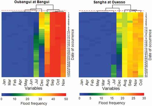
Figure A2. Seasonal similarity between Kutu muke and Chembe ferry. The red dashed line indicates the cut in the tree clustering months in which floods occurred often and months in which floods happen seldom or never. Vertical axes display months with daily frequency within the concerned cell, coloured on the horizontal axis to associate the date of occurrence with flood frequency. Flood frequency values are expressed in terms of relative frequency (%).

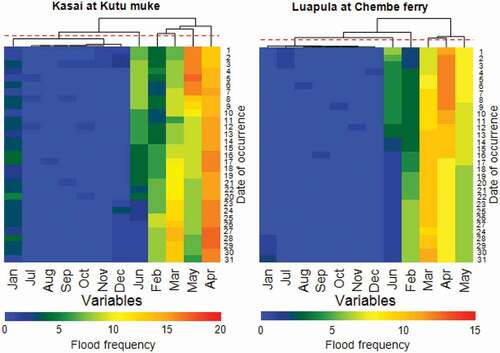
Figure A3. Seasonal dissimilarity between Kinshasa and Kisangani. The red dashed line indicates the cut in the tree clustering months in which floods occurred often and months in which floods happen seldom or never. Vertical axes display months with daily frequency within the concerned cell, coloured on the horizontal axis to associate the date of occurrence with flood frequency. Flood frequency values are expressed in terms of relative frequency (%).

References

- Addinsoft. 2021. XLSTAT statistical and data analysis solution. New York, USA. Available from: https://www.xlstat.com
- Alsdorf, D., et al., 2016. Opportunities for hydrologic research in the Congo Basin. Reviews of Geophysics, 54, 378–409. doi:10.1002/2016RG000517
- Assani, A.A., et al., 2006. Comparison of impacts of dams on the annual maximum flow characteristics in three regulated hydrologic regimes in Quebec (Canada). Hydrological Processes, 20, 3485–3501. doi:10.1002/hyp.6150
- Axt, I. and Fried, R., 2020. On variance estimation under shifts in the mean. AStA Advances in Statistical Analysis, 104, 417–457. doi:10.1007/s10182-020-00366-5
- Bačová-Mitková, V. and Onderka, M., 2010. Analysis of extreme hydrological events on THE Danube using the peak over threshold method. Journal of Hydrology and Hydromechanics, 58, 88–101. doi:10.2478/v10098-010-0009-x
- Bayliss, A.C. and Jones, R.C., 1999. Peaks-over-threshold flood database: summary statistics and seasonality. Report - Institute of Hydrology (United Kingdom).
- Bernhofen, M.V., et al., 2021. Global flood exposure from different sized rivers. Natural Hazards and Earth System Sciences Discussions, 1–25. doi:10.5194/nhess-2021-102
- Beyene, T., Ludwig, F., and Franssen, W., 2013. The potential consequences of climate change in the hydrology regime of the Congo River Basin. In: A. Haensler, et al., eds. Climate Change Scenarios for the Congo Basin. Hamburg, Germany: Climate Service Centre Report No. 11. 2192–4058.
- Bischiniotis, K., et al., 2018. The influence of antecedent conditions on flood risk in Sub-Saharan Africa. Natural Hazards and Earth System Sciences, 18 (1), 271–285. doi:10.5194/nhess-18-271-2018
- Black, A.R. and Werritty, A., 1997. Seasonality of flooding: a case study of North Britain. Journal of Hydrology, 195 (1), 1–25. doi:10.1016/S0022-1694(96)03264-7
- Bola, G., et al., 2022. Multireturn periods flood hazards and risks assessment in the Congo River Basin. In: R.M. Tshimanga, G.D. Moukandi N’kaya, and D. Alsdorf, eds., Congo basin hydrology, climate, and biogeochemistry: a foundation for the future, geophysical monograph 269, First Edition, English Version. © 2022 American Geophysical Union. Published 2022 by John Wiley & Sons, Inc. doi:10.1002/9781119657002.ch27
- Brolsma, J.U., 2010. PIANC, The World Association for Waterborne Transport Infrastructure, an association in a changing world [online]. Boulevard Albert: PIANC. Available from: https://www.pianc.org/about [ Accessed 25th August 2021].
- Brummett, R. et al., 2009. Water resources, forests and ecosystem goods and services. In: C. de Wasseige, et al., eds. The Forests of the Congo Basin - State of the Forest 2008. Luxembourg: Publications Office of the European Union,141–157.
- Burn, D.H., 1997. Catchment similarity for regional flood frequency analysis using seasonality measures. Journal of Hydrology, 202, 212–230. doi:10.1016/S0022-1694(97)00068-1
- Burn, D.H. and Arnell, N.W., 1993. Synchronicity in global flood responses. Journal of Hydrology, 144, 381–404. doi:10.1016/0022-1694(93)90181-8
- Chen, L., et al., 2013. A new method for identification of flood seasons using directional statistics. Hydrological Sciences Journal, 58 (1), 28–40. doi:10.1080/02626667.2012.743661
- Collins, M.J., et al., 2014. Annual floods in New England (USA) and Atlantic Canada: synoptic climatology and generating mechanisms. Physical Geography, 35, 195–219. doi:10.1080/02723646.2014.888510
- Collins, M.J., 2018. River flood seasonality in the Northeast United States: characterization and trends. Physical Geography, 35, 195–219. doi:10.1080/02723646.2014.888510
- Collins, M.J., 2019. River flood seasonality in the Northeast United States: characterization and trends. Hydrological Processes, 33, 687–698. doi:10.1002/hyp.13355
- Creese, A., Washington, R., and Jones, R., 2019. Climate change in the Congo Basin: processes related to wetting in the December–February dry season. Climate Dynamics, 53, 3583–3602. doi:10.1007/s00382-019-04728-x
- Cunderlik, J. and Burn, D., 2002. The use of flood regime information in regional flood frequency analysis. Hydrological Sciences Journal, 47, 77–92. doi:10.1080/02626660209492909
- Cunderlik, J.M., Ouarda, T.B.M.J., and Bobée, B., 2004a. Determination of flood seasonality from hydrological records/Détermination de la saisonnalité des crues à partir de séries hydrologiques. Hydrological Sciences Journal, 49, null–526. doi:10.1623/hysj.49.3.511.54351
- Cunderlik, J.M., Ouarda, T.B.M.J., and Bobée, B., 2004b. On the objective identification of flood seasons. Water Resources Research, 40. doi:10.1029/2003WR002295
- Dettinger, M.D. and Diaz, H.F., 2000. Global characteristics of stream flow seasonality and variability. Journal of Hydrometeorology, 1, 289–310. 10.1175/1525-7541(2000)001<0289:GCOSFS> 2.0.CO;2. doi:10.1175/1525-7541(2000)001<0289:GCOSFS>2.0.CO;2
- Engeland, K., et al., 2018. Use of historical data in flood frequency analysis: a case study for four catchments in Norway. Hydrology Research, 49, 466–486. doi:10.2166/nh.2017.069
- Ficchì, A. and Stephens, L., 2019. Climate variability alters flood timing across Africa. Geophysical Research Letters, 46 (15), 8809–8819. doi:10.1029/2019GL081988.
- Fisher, N.I., 1993. Statistical analysis of circular data. Cambridge, UK: Cambridge University Press.
- GRDC, 2020. Operating the global runoff database [online]. Global Runoff Data Centre. Available from: https://www.bafg.de/GRDC/EN/03_dtprdcts/dataproducts_node.html [ Accessed 22th August 2020].
- Hall, J., et al., 2014. Understanding flood regime changes in Europe: a state of the art assessment. Hydrology and Earth System Sciences, 18, 2735–2772. doi:10.5194/hess-18-2735-2014
- Hall, J. and Bloschl, G., 2018. Spatial patterns and characteristics of flood seasonality in Europe, hydrol. Hydrology and Earth System Sciences, 22, 3883–3901. doi:10.5194/hess-22-3883-2018
- Hannaford, J. and Buys, G., 2012. Trends in seasonal river flow regimes in the UK. Journal of Hydrology, 475, 158–174. doi:10.1016/j.jhydrol.2012.09.044
- Hart, J.A., 2000. Impact and sustainability of indigenous hunting in the Ituri forest, Congo-Zaïre: a comparison of unhunted and hunted duiker populations. In: J.G. Robinson and E.L. Bennet, eds. Hunting for sustainability in tropical forests. New York: Columbia University Press, 106–153.
- Hawker, A., et al., 2020. Comparing earth observation and inundation models to map frequent to rare flood hazards. ERL-108837, Environmental Research Letters, 15 (12), 124032. doi:10.1088/1748-9326/abc216
- Hirabayashi, Y., et al., 2013. Global flood risk under climate change. Nature Climate Change, 3, 816–821. doi:10.1038/nclimate1911
- Hölscher, D., et al., 1997. Evaporation from young secondary vegetation in eastern Amazonia. Journal of Hydrology, 193, 293–305. doi:10.1016/S0022-1694(96)03145-9
- Impreza-Servisi-Coordinati, 2010. Conseil agricole et rural de gestion (CARG) du Territoire d’Inongo: plan de développement agricole et rural du territoire. Impreza-Servisi-Coordinati, Projet de Développement Agricole du Bandundu [online]. Ministère de l’Agriculture, Pêche et Élevage, République Démocratique du Congo. Financement Union Européenne. Food, 172, 355. Available from: https://docplayer.fr/114436847-Conseil-agricole-et-rural-de-gestion-carg-du-territoire-de-inongo-plan-de-developpement-agricole-et-rural-du-territoire.html
- Ingram, V., 2009. The hidden costs and values of NTFP exploitation in the Congo Basin [online]. Buenos Aires, Argentina: FAO. Available from: https://www.cifor.org/knowledge/publication/3034, [ Accessed 12th March 2021].
- Janowiak, J.E., 1988. An investigation of interannual rainfall variability in Africa. Journal of Climate, 1, 240–255. doi:10.1175/1520-0442(1988)001 <0240:AIOIRV>2.0.CO;2
- Kiem, A.S., Franks, S.W., and Kuczera, G., 2003. Multi-decadal variability of flood risk, 825 Geophys. Geophysical Research Letters, 30, 1035. 2. doi:10.1029/2002GL015992
- Kundzewicz, Z.W., et al., 2014. Flood risk and climate change: global and regional perspectives. Hydrological Sciences Journal, 59, 1–28. doi:10.1080/02626667.2013.857411
- Laraque, A., et al., 1998. Origine des variations de débits du Congo à Brazzaville durant le 20ème siècle. In: E. Servat, et al., eds. Water resources variability in Africa during the 20th century = Variabilité des ressources en eau en Afrique au 20ème siècle, Publication - AISH. Wallingford: AISH, 171–179.
- Laraque, A., et al., 2001. Spatiotemporal variations in hydrological regimes within Central Africa during the XXth century. Journal of Hydrology, 245, 104–117. doi:10.1016/S0022-1694(01)00340-7
- Lecce, S.A., 2000. Seasonality of flooding in North Carolina. Southeastern Geographer, 40 (2), 168–175. Available from: http://www.jstor.org/stable/44371080
- Levene, H.O., 1960. Robust tests for equality of variances. In: Contributions to probability and statistics. Stanford: Stanford University Press 278292, Chapter 25.
- Liu, P., et al., 2010. Flood season segmentation based on the probability change-point analysis technique. Hydrological Sciences Journal/Journal Des Sciences Hydrologiques, 55, 540–554. doi:10.1080/02626667.2010.481087
- Magilligan, F.J. and Nislow, K.H., 2005. Changes in hydrologic regimes by dams. Geomorphology, 71, 61–78. doi:10.1016/j.geomorph.2004.08.017
- Mangini, W., et al., 2018. Detection of trends in magnitude and frequency of flood peaks across Europe. Hydrological Sciences Journal, 63, 493–512. doi:10.1080/02626667.2018.1444766
- Mardia, K.V., 1975. Statistics of directional data. Journal of the Royal Statistical Society. Series B (Methodological), 37 (3), 349–393 (45). doi:10.1111/j.2517-6161.1975.tb01550.x
- McHugh, M.J. and Rogers, J.C., 2001. North Atlantic oscillation influence on precipitation variability around the Southeast African Convergence Zone. Journal of Climate, 14, 3631–3642. doi:10.1175/1520-0442(2001)014 <3631:NAOIOP>2.0.CO;2
- Mertz, B., et al., 2018. Spatial coherence of flood-rich and flood-poor periods across Germany. Journal of Hydrology, 559, 813–826. doi:10.1016/j.jhydrol.2018.02.082
- Minasny, B. and Hartemink, A.E., 2011. Predicting soil properties in the tropics. Earth-Science Reviews, 106, 52–62. doi:10.1016/j.earscirev.2011.01.005
- Munzimi, Y.A., et al., 2015. Characterizing Congo Basin rainfall and climate using Tropical Rainfall Measuring Mission (TRMM) satellite data and limited rain gauge ground observations. Journal of Applied Meteorology and Climatology, 54 (3), 541–555. doi:10.1175/JAMC-D-14-0052.1
- Nicholson, S.E., 2000. The nature of rainfall variability over Africa on time scales of decades to millenia. Global and Planetary Change, 26 (1–3), 137–158. doi:10.1016/S0921-8181(00)00040-0
- Nicholson, S.E., Funk, C., and Fink, A.H., 2018. Rainfall over the African continent from the 19th through the 21st century. Global and Planetary Change, 165, 114–127. doi:10.1016/j.gloplacha.2017.12.014
- Obasi, G., 2005. The impacts of ENSO in Africa. Climate Change and Africa, 218–230. doi:10.1017/CBO9780511535864.030
- Olivry, J.C. and Et Boulègue, J., 1995. Grands bassins fluviaux Périatlantiques: Congo, Niger, Amazone: actes du colloque PEGI INSU - CNRS – ORSTOM. du 22 au 24 novembre 1993, 0767-2896. Paris, France: ORSTOM Éditions 1995.
- Ouarda, T.B.M.J., Ashkar, F., and El‐Jabi, N., 1993. Peaks over threshold model for seasonal flood variations. Engineering Hydrology, 341–346.
- Ouarda, T.B.M.J., et al., 2000. Regional flood peak and volume estimation in Northern Canadian Basin. Journal of Cold Regions Engineering, 14, 176–191. doi:10.1061/(ASCE)0887-381X(2000)14:4(176)
- Ouarda, T.B.M.J., et al., 2006. Data-based comparison of seasonality-based regional flood frequency methods. Journal of Hydrology, Hydro-ecological Functioning of the Pang and Lambourn Catchments, UK, 330, 329–339. doi:10.1016/j.jhydrol.2006.03.023
- Poff, N.L., 2018. Beyond the Natural Flow Regime? Broadening the hydro-ecological foundation to meet environmental flows challenges in a nonstationary world. Freshwater Biology, 63, 1011–1021. doi:10.1111/fwb.13038
- Pokam, W.M. et al., 2014. Identification of processes driving low-level westerlies in west equatorial Africa. Journal of Climate, 27 (11), 4245–4262.
- Qiang, F., Zhong, T., and Wei Wang, W., 2018. Study on risk assessment and early warning of flood-affected areas when a dam break occurs in a mountain river. Water, 10, 1369. doi:10.3390/w10101369.
- Reliefweb, Office for the Coordination of Humanitarian Affairs (OCHA), 2019. Washington, DC: United Nations Office for the Coordination of Humanitarian Affairs. Available from: https://reliefweb.int/disaster/fl-2019-000160-cog [Accessed 22 Apr 2020].
- Rogers, J.C., 1997. North Atlantic storm track variability and its association to the North Atlantic Oscillation and climate variability of northern Europe. Journal of Climate, 10 (7), 1635–1647. doi:10.1175/1520-0442(1997)010<1635:nastva>2.0.co;2
- Runge, J. and Nguimalet, C.-R., 2005. Physiogeographic features of the Oubangui catchment and environmental trends reflected in discharge and floods at Bangui 1911–1999, Central African Republic. Geomorphology, Tropical Rivers, 70, 311–324. doi:10.1016/j.geomorph.2005.02.010
- Schmocker-Fackel, P. and Naef, F., 2010. Changes in flood frequencies in Switzerland since 1500. Hydrology and Earth System Sciences, 14 (8), 1581–1594. doi:10.5194/hess-14-1581-2010
- SO-HYBAM, 2020. Amazon basin water resources observation services. Available from: https://hybam.obs-mip.fr [ Accessed 22th August 2020].
- Solari, S., et al., 2017. Peaks over threshold (POT): a methodology for automatic threshold estimation using goodness of fit p-value. Water Resources Research, 53, 2833–2849. doi:10.1002/2016WR019426
- Stat. Soft. Inc, 2004. STATISTICA (data analysis software system), Version 7. Available from: www.statsoft.com
- Steirou, E.-S., et al., 2017. Links between large-scale circulation 899 patterns and streamflow in Central Europe: a review. Journal of Hydrology, 549, 484–900 500— . doi:10.1016/j.jhydrol.2017.04.003
- Svensson, C., Kundzewicz, W.Z., and Maurer, T., 2005. Trend detection in river flow series: 2. Flood and low-flow index series/Détection de tendance dans des séries de débit fluvial: 2. Séries d’indices de crue et d’étiage. Hydrological Sciences Journal, 50, null–824. doi:10.1623/hysj.2005.50.5.811
- Svensson, C., et al., 2006. Trends in river floods: why is there no clear signal in observations? In: Frontiers in flood research, 8th Kovacs Colloquium, UNESCO, Paris, 30 June–1 July 2006. IAHS, 1–18.
- Talbot, C.J., et al., 2018. The impact of flooding on aquatic ecosystem services. Biogeochemistry, 141, 439–461. doi:10.1007/s10533-018-0449-7
- Talling, P.J., et al., 2022. Flood and tides trigger longest measured sediment flow that accelerates for thousand kilometers into deep-sea. Nature Communications (under review).
- Teugels, G.G. and Thieme, M.L., 2005. Freshwater fish biodiversity in the Congo Basin. In: M.L. Thieme, et al., eds. Freshwater ecoregions of Africa and Madagascar: a conservation assessment. Washington, DC: Island Press, 51–53.
- Todd, M. and Washington, R., 2004. Climate variability in central equatorial Africa: influence from the Atlantic sector. Geophysical Research Letters, 31 (23), L23202. 00948276 31. doi:10.1029/2004GL020975
- Tramblay, Y., et al., 2021. On the influence of extreme rainfall and antecedent soil moisture on flood hazards in Africa. EGU General Assembly, EGU21–2908. Online. doi:10.5194/egusphere-egu21-2908 [19–30 Apr 2021].
- Trigg, M.A., et al., 2022. Putting river users at the heart of hydraulics and morphology research in the Congo Basin. In: R.M. Tshimanga, G.D. Moukandi N’kaya, and D. Alsdorf, eds. Congo Basin Hydrology, Climate, and Biogeochemistry: A Foundation for the Future, Geophysical Monograph 269, first edition, English version. © 2022 American Geophysical Union. Published 2022 by John. Wiley & Sons, Inc. doi:10.1002/9781119657002.ch28
- Tshimanga, R.M. and Hughes, D.A., 2012. Climate change and impacts on the hydrology of the Congo Basin: the case of the northern sub-basins of the Oubangui and Sangha Rivers. Physics and Chemistry of the Earth, Parts A/B/C, 50–52, 72–83. doi:10.1016/j.pce.2012.08.002
- Tshimanga, R. and Hughes, D., 2014. Basin-scale performance of a semidistributed rainfall-runoff model for hydrological predictions and water resources assessment of large rivers: the Congo River. Water Resources Research, 50, 1174–1188. doi:10.1002/2013WR014310
- Tshimanga, R.M., et al., 2016. A regional perceptive of flood forecasting and disaster management systems for the Congo River Basin. In: T.E. Adams and T.C. Pagano, eds. Flood forecasting. Academic Press, Chapter 4, 87–124. doi:10.1016/B978-0-12-801884-2.00004-9
- Tshimanga, R.M., et al., 2022. Towards a framework of catchment classification for hydrologic predictions and water resources management in the ungauged basin of the Congo River: an a priori approach. In: R.M. Tshimanga, G.D. Moukandi N’kaya, and D. Alsdorf, eds. Congo basin hydrology, climate, and biogeochemistry: a foundation for the future, geophysical monograph 269, first edition, english version. © 2022 American Geophysical Union. Published 2022 by John. Wiley & Sons, Inc. doi:10.1002/9781119657002.ch24
- Warner, J., et al., 2019. The fantasy of the grand inga hydroelectric project on the river Congo. Water, 11 (3), 407. doi:10.3390/w11030407
- Washington, R., et al., 2013. Congo Basin rainfall climatology: can we believe the climate models? Philosophical Transactions of the Royal Society B: Biological Sciences, 368, 20120296. doi:10.1098/rstb.2012.0296
- Wesselink, A.J., et al., 1996. Les régimes hydroclimatiques et hydrologiques d’un bassin versant de type tropical humide : l’Oubangui (République Centrafricaine). In: P. Chevallier and B. Pouyaud eds. L'hydrologie tropicale : géosciences et outil pour le développement : mélanges à la mémoire de Jean Rodier. Wallingford: AISH, 179–194. (Publication - AISH ; 238). Journées Hydrologiques de l'ORSTOM : Conférence de Paris, 11., Paris (FRA), 1995/05/02-04.
- Wilkinson, L. and Friendly, M., 2009. The history of the cluster heat map. The American Statistician, 63 (2), 179–184. doi:10.1198/tas.2009.0033
- Wohl, E., et al., 2012. The hydrology of the humid tropics. Nature Climate Change, 2 (9), 655–662. doi:10.1038/nclimate1556
- Wold, H., 1975. Path models with latent variables: the NIPALS Approach. **NIPALS = Nonlinear Iterative PArtial Least Squares. In: H.M. Blalock, et al., eds. International perspectives on mathematical and statistical modeling,quantitative sociology. Academic Press, 307–357. doi:10.1016/B978-0-12-103950-9.50017-4
- Ye, S., et al., 2017. Understanding flood seasonality and its temporal shifts within the contiguous United States. Journal of Hydrometeorology, 18 (7), 1997–2009. doi:10.1175/JHM-D-16-0207.1
- Yujian, L. and Liye, X., 2010. Unweighted multiple group method with arithmetic mean. In: 2010 IEEE fifth international conference on Bio-Inspired Computing: Theories and Applications (BIC-TA). Presented at the 2010 IEEE fifth international conference on Bio-Inspired Computing: Theories and Applications (BIC-TA), 830–834. doi:10.1109/BICTA.2010.5645232