Changes in rain-on-snow events in mountain catchments in the rain–snow transition zone

ABSTRACT

A shift from snowfall to rain affecting snow storage is expected in future. Consequently, changes in rain-on-snow (ROS) events may occur. We evaluated the frequency and trends in ROS events and their runoff responses at different elevations related to changes in climate variables. We selected 40 central European mountain catchments located in the rain–snow transition zone, and used a conceptual catchment model to simulate runoff components for the period 1965–2019. The results showed large temporal and spatial differences in ROS events and their respective runoff responses across individual study catchments and elevations, with primarily an ROS increase at highest elevations and a decrease at lower elevations during spring. ROS events contributed 3–32% to the total seasonal direct runoff. The detected trends reflect changes in climate and snow variables, with an increase in air temperature resulting in the decrease in snowfall fraction and shorter snow cover period.

KEYWORDS:

• rain-on-snow events
• rain-on-snow variability
• rain-on-snow trends
• rain–snow transition zone
• climate change

Editor A. Castellarin; Associate Editor S. Kampf

1 Introduction

Seasonal snowpack significantly influences catchment runoff and thus represents an important component of the hydrological cycle. Moreover, snowpack accumulated during the cold season affects groundwater recharge and thus influences spring runoff and summer low flows (Hammond et al. 2018, Jenicek and Ledvinka 2020, Vlach et al. 2020). Predicted changes in climate variables will have a strong impact on hydrometeorological processes including snow storage and snowmelt dynamics (Jennings et al. 2018, Sezen et al. 2020). Additionally, changes in precipitation intensity and distribution, as well as a shift from snowfall to rain, are expected (Serquet et al. 2011, Musselman et al. 2018, Blahusiakova et al. 2020, Li et al. 2020). These changes, among others, affect rain-on-snow (ROS) events, which are considered to be one of the major causes of winter floods in many regions (Pradhanang et al. 2013, Würzer et al. 2017, Brunner et al. 2019) and which may occur more frequently in the future (Freudiger et al. 2014, Jennings et al. 2018, Musselman et al. 2018). Due to their complex and still not fully understood behaviour, ROS events are considered to be one of the major unsolved problems in hydrology (Blöschl et al. 2019). According to Il Jeong and Sushama (2017), 80% of the annual January to May maximum daily runoff is associated with ROS for large parts of Northern America. Moreover, it is still not clear how climate change will affect ROS occurrence due to its complex nature (Sezen et al. 2020). Changes in the frequency and intensity of ROS events in a warming climate may vary temporally and spatially, reflecting changes in snow cover and the amount of rain, while projections reveal a decrease in snow storage for all elevations, time periods and emission scenarios (Marty et al. 2017, Notarnicola 2020, Jenicek et al. 2021).

There is still considerable uncertainty regarding how the frequency of ROS events will change with temperature increase, while peak streamflow caused by ROS is predicted to increase due to more rapid melting from enhanced energy inputs, and a warmer snowpack during future ROS (López-Moreno et al. 2021). Potential ROS changes can be also attributed to changes in the occurrence of dominant weather patterns leading to ROS events, or to variations of the freezing point line (Krug et al. 2020, Ohba and Kawase 2020). Beniston and Stoffel (2016) revealed that the number of ROS events could increase by 50% as an initial response to a temperature increase of 2–4°C compared to the present, but decline thereafter when the air temperature increase exceeds 4°C. The same study showed that the temperature increase observed in northeastern Switzerland for the 1960–2015 period has contributed directly to the increase in the number of ROS events by about 40% at low elevations, and by 200% at high elevations. Results of other recent studies, however, showed that the number of ROS events is expected to decrease in low- and mid-latitude regions by reducing the number of days with snow cover on the ground (Mccabe et al. 2007, Surfleet and Tullos 2013, Musselman et al. 2018, Li et al. 2019, López-Moreno et al. 2021). In contrast, ROS events are predicted to occur more frequently in the future due to an increase in the number of days with rain in both high-elevation and high-latitude regions (Surfleet and Tullos 2013, Il Jeong and Sushama 2017, Trubilowicz and Moore 2017, Musselman et al. 2018, Li et al. 2019). Future projections for the humid mountain regions suggest an overall ROS increase in the middle of the winter season (from November to March) since more precipitation will fall as rain rather than snow (Il Jeong and Sushama 2017). In contrast, a decrease in ROS is expected for early and late winter due to the shortening of the period with existing snow cover on the ground (Sezen et al. 2020). Similar changes may occur in many regions that experience both snow and rain during winter months (Cohen et al. 2015). A broader area is expected to become vulnerable to changes in ROS in the future, as future climate projections show an increase in the frequency and areal extent of ROS, including many parts of the Arctic over the next 50 years (Rennert et al. 2009).

An assessment of changes in ROS events for large areas should be preceded by a detailed analysis of all processes and influencing factors affecting ROS situations. Several recent studies have attempted to better understand these processes and factors for larger areas. The results of Würzer et al. (2016) for the Swiss Alps demonstrated the strong influence of initial snowpack properties on runoff formation during ROS, indicating that the retention capacity of the snowpack is crucial during ROS events (Garvelmann et al. 2015, Brandt et al. 2022). Nevertheless, not all ROS events generate direct runoff, since the snowpack can store a large amount of incoming rainwater (Wayand et al. 2015, Juras et al. 2021). Therefore, one important issue is to properly understand rainwater behaviour in the snowpack (Surfleet and Tullos 2013, Juras et al. 2017, Würzer et al. 2017). Another important issue is to consider ROS events in the context of the entire snowpack energy balance, which controls overall snowmelt amount and dynamics (Brandt et al. 2022). Although the heat supplied by the rain during ROS usually contributes rather a minor energy source for snowmelt – usually up to 10% of the total energy balance at longer temporal resolutions (Mazurkiewicz et al. 2008, Trubilowicz and Moore 2017, Li et al. 2019) – rain heat input is more important for snowmelt generation at shorter temporal resolutions (Hotovy and Jenicek 2020). The heat from rain may contribute more than 25% of the total energy accessible for melt during days with heavy rain (Jennings and Jones 2015, Hotovy and Jenicek 2020), resulting in faster snowmelt and consequently related to a higher flood risk. Furthermore, rainfall events are often associated with additional turbulent (sensible and latent) heat input (Marks et al. 1998, Garvelmann et al. 2014), and longwave radiation that can speed up snowmelt as well (Sezen et al. 2020).

The interaction of different influencing factors makes it difficult to accurately predict the effect of snow cover on runoff formation for an upcoming ROS event (Würzer et al. 2016). Most ROS studies use similar approaches, for example they are event based and region specific (Li et al. 2019). Although ROS events have been a focus for hydrologists over the last several decades, the physical complexity and associated impacts of ROS has led to varying definitions and methods applied in their assessments (Pall et al. 2019). For example, various threshold values for air temperature, total precipitation, snowpack and runoff characteristics are used for ROS event definition (Freudiger et al. 2014, Würzer et al. 2016, Bieniek et al. 2018, Crawford et al. 2020, Brandt et al. 2022). Studies performed in different regions around the world have reported a wide range (4–75%) of snowmelt contribution to runoff during ROS (Li et al. 2019), thus, any regional comparison is complicated. The quantification of ROS, and the assessment of their changes, is also made difficult because ROS events generally occur at higher elevations and/or latitudes, which typically have sparse observation networks (Pall et al. 2019). Therefore, several studies employed modelling approaches as suitable tools to detect ROS events (Mazurkiewicz et al. 2008, Wayand et al. 2015, Beniston and Stoffel 2016, Wever et al. 2016, Würzer and Jonas 2018), or to predict changes in the ROS occurrence reflecting existing climate projections implemented into hydrological models (Bieniek et al. 2018, Ohba and Kawase 2020).

Although several studies have focused on changes in ROS frequency and intensity, trend analysis of both ROS occurrence and related runoff response is rather scarce. Most of these studies, furthermore, were done at a catchment scale with limited focus on elevation, which highly influences precipitation phase and snow cover. Additionally, most of the central European studies were done in the region of the Alps, while studies performed in other, usually lower elevation mountain ranges are rare. The focus on lower elevation mountain ranges is, however, important since they represent areas in rain–snow transition zones with typically large changes in snow storage, affecting ROS occurrence (Freudiger et al. 2014, Juras et al. 2021, Nedelcev and Jenicek 2021). Understanding the spatial distribution, temporal variability, and influencing drivers causing ROS in a changing climate is critically important to better predict these events and to create strategies to mitigate their effects on the terrestrial ecosystems and society (Bieniek et al. 2018, Brandt et al. 2022).

To fill this research gap, the objectives of this study were (1) to evaluate the frequency and ongoing trends in ROS events at different elevations and to relate them to changes in climate variables, and (2) to analyse changes in runoff responses related to ROS events. We selected 40 near-natural central European mountain catchments located in rain–snow transition zones with significant snow influence on runoff. Our study benefits from long time series (1965–2019) of daily meteorological and hydrological variables, which enabled us to simulate several components of the water cycle for different elevations using a semi-distributed conceptual model.

2 Material and methods

2.1 Study area and data monitoring

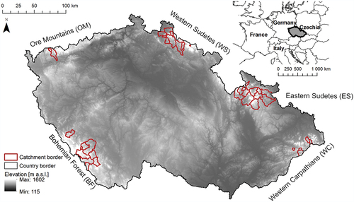
The study was performed for 40 catchments located in five mountain ranges in Czechia (Fig. 1). The same set of study catchments was used in Nedelcev and Jenicek (2021). Selected characteristics of all study catchments are listed in Table S1 in the Supplementary material. Mountain catchments with near-natural streamflow, with snow influence on runoff and with no major human influences were selected. Additionally, the availability of long-term time series of hydrological and meteorological data were an important criterion for the selection. We used time series of daily precipitation and daily mean air temperature, both for the period 1965–2019, and mean daily discharge and weekly snow water equivalent (SWE), both for the period 1980–2014. All data were available from 22 meteorological stations and 40 hydrological stations operated by the Czech Hydrometeorological Institute (CHMI) and were further used in a hydrological model, described in the next section. Station and modelled data together enabled the analysis of 55 seasons from 1965 to 2019, where one season represents a hydrological year (1 November–31 October).

Figure 1. Location of the 40 study catchments, located in five mountain ranges in Czechia (Nedelcev and Jenicek 2021).

2.2 HBV-light model

A semi-distributed bucket-type Hydrologiska Byråns Vattenbalansavdelning model (Lindström et al. 1997) in its software implementation “HBV-light” (Seibert and Vis 2012) was used to simulate individual components of the rainfall–runoff process, including direct runoff and baseflow. Each study catchment was divided into elevation zones at intervals of 100 m, for which all input data at a daily resolution were distributed using calibrated lapse rates for both air temperature and precipitation. The HBV model consists of four basic routines – a snow routine, soil routine, groundwater routine, and routing function to simulate catchment runoff – based on time series of observed daily mean air temperature, daily precipitation and monthly potential evapotranspiration calculated using the temperature-based method defined by Oudin et al. (2005). The details of the model structure can be found in Seibert and Vis (2012) or Girons Lopez et al. (2020).

The calibration and validation of the model were originally done for previous studies which share the same set of study catchments (Jenicek and Ledvinka 2020, Jenicek et al. 2021). We thus provide the basic description here and refer readers to the above studies for a more detailed description of the procedure. The HBV model was calibrated automatically for each of the study catchments against observed daily runoff and weekly SWE for the calibration period 1980–1997, using a genetic optimization algorithm (Seibert 2000). One hundred optimized parameter sets resulting from 100 calibration trials were derived and further used to create 100 simulations for each catchment. Finally, a median simulation for each catchment was calculated and used for the following analyses. The model was validated for the period 1998–2014.

A combination of several objective criteria was used to evaluate the goodness of fit of the model: (1) logarithmic Nash-Sutcliffe efficiency for runoff (Nash and Sutcliffe 1970) with 60% weight, (2) Nash-Sutcliffe efficiency for SWE with 20% weight, and (3) volume error with 20% weight. These three criteria were weighted to calculate the resulting objective function of the model.

The results of model calibration and testing were detailed in Jenicek et al. (2021) and Nedelcev and Jenicek (2021). These studies showed the model’s ability to correctly simulate SWE and runoff including existing trends in time series. In this new study, we additionally provide throughout an assessment of the model’s ability to simulate SWE and snowmelt related to ROS events (Section 3.1 and Supplementary material, Figs S1–S5).

2.3 Definition of ROS days and events

Several selection criteria were defined to identify individual ROS days and ROS events that may occur during periods with snow cover and rainfall occurrence. Here, we distinguished between an ROS day and an ROS event as follows.

An ROS day was identified when the three following threshold conditions were fulfilled: (1) the daily mean air temperature was higher than 0°C, determining whether precipitation falls as rain or snowfall; (2) SWE was higher than 10 mm, ensuring that a sufficiently thick snowpack layer is on the ground; and (3) the rainfall intensity exceeded 5 mm d to avoid negligible amounts of rain or drizzle. The HBV model simulates the three above variables both at a catchment scale and for individual elevation zones, which enabled an analysis of the occurrence of ROS days for each elevation zone across the whole study area.

Unlike the ROS day, the ROS event may include both ROS days and non-ROS days. The duration of the ROS event is calculated from the initial ROS day (Q₁; the first day when all three of the above threshold criteria were fulfilled) to the last day (Q_last), the day when the maximum simulated runoff was reached. We set the maximum response time to six days, similar to Freudiger et al. (2014), to avoid multiple runoff events or long runoff responses caused by multiple interactions (e.g. first rain and then long periods of above-zero temperatures causing snowmelt). Since an ROS event was defined based on the simulated runoff, the related analysis of runoff responses was performed at a catchment scale only.

2.4 Runoff classes and hydrological response calculation

Detected ROS events were divided into four runoff classes (Table 1) based on the change of simulated runoff between the day preceding the first ROS day (Q₀, zero day) and the day with the maximum event runoff (Q_last), to access the intensity of individual hydrological responses. A similar runoff classification was used in Juras et al. (2021).

Table 1. Classification of ROS event runoff response. Q₀ represents daily runoff on the day preceding the first ROS day of the specific ROS event, and Q_last represents simulated daily runoff on the last day of the specific ROS event (defined as the day with maximum runoff).

Runoff class	Hydrological response	Definition
1	Negligible runoff	Qlast ≤ 125% Q0
2	Low runoff	125% Q0 < Qlast ≤ 250% Q0
3	Medium runoff	250% Q0 < Qlast ≤ 500% Q0
4	High runoff	Qlast > 500% Q0

Here, we assigned an ROS event as class 1 (negligible runoff) if simulated runoff on the last day did not exceed 125% of simulated runoff on the zero day; as class 2 (low runoff) if simulated runoff on the last day exceeded 125% but did not exceed 250% of simulated runoff on the zero day; as class 3 (medium runoff) if simulated runoff on the last day exceeded 250% but did not exceed 500% of simulated runoff on the zero day; and as class 4 (high runoff) if simulated runoff on the last day was higher than 500% of simulated runoff on the zero day.

Additionally, total direct (event) runoff Q_event (mm) was calculated for each ROS event to access the change of the hydrological response to ROS (Equation (1)(1) $Q_{event}=\sum _{t=1}^N(Q\left(t\right)-Q_{base}\left(t\right))$(1) ).

(1) $Q_{event}=\sum _{t=1}^N(Q\left(t\right)-Q_{base}\left(t\right))$(1)

where Q (mm d⁻¹) is simulated runoff on day t and Q_base (mm d⁻¹) is baseflow runoff simulated by the HBV model as an outflow from the lowest groundwater box. N represents the number of days of the ROS event and t is iterated over the first to the last day of the ROS event.

2.5 Trend analysis

The Mann-Kendall test (Mann 1945, Kendall 1975) was used to analyse the univariate time series for the presence of statistically significant trends of various ROS-related variables for the study period 1965–2019. The presence of a consistently decreasing or increasing temporal trend was tested using the Mann-Kendall test p value. The p value was calculated based on the 55-year data series (1965–2019) with two different trend significance threshold levels, of .1 and .05. The Theil-Sen’s slope estimator was used to assess the monotonic trend slope (Sen 1968), expressing the change in variables per defined time period (decade).

3 Results

3.1 Model calibration and testing

For model calibration and validation, it was important to ensure that the model correctly simulates both SWE and runoff during ROS events. All results from this analysis are shown in the Supplementary material (Figs S1–S5).

Overall model performance was assessed using several objective functions, showing the median model efficiency for runoff using a logarithmic Nash-Sutcliffe criterion equal to 0.67 for model calibration and 0.61 for model validation (Fig. S1). The median runoff volume error reached 1.0 for calibration (i.e. perfect fit) and 0.90 for validation. The median model efficiency for SWE was 0.70 for model calibration and 0.72 for model validation (Fig. S1). We also assessed how 100 model parameterizations impacted the results (Fig. S2). Results showed that median simulations resulted in close-to-median numbers of ROS days in individual catchments. In addition, the accuracy of the SWE simulations was further assessed for both ROS and non-ROS days (Fig. S3), which did not show any major inconsistencies in the SWE simulations. More detailed testing of SWE simulations was carried out by Jenicek et al. (2021) and Nedelcev and Jenicek (2021), who worked with the same set of catchments as used in our study.

The model slightly underestimated the number of ROS days in individual catchments; however, the differences were not large (Fig. S4). Comparison of simulated and observed ROS event classification, defined in Section 2.4, showed that 4180 out of 7428 ROS events (54%) were assigned the same class, 27% were overestimated (simulated runoff class was higher than observed), and 19% were underestimated (simulated runoff class was lower than observed) (Fig. S5).

3.2 ROS day occurrence

At a catchment scale, we identified a total of 15 894 ROS days in all 40 catchments during the study period, 1965–2019. It is worth noting that ROS days usually occurred at the same time at multiple catchments and elevation zones, but ROS days were analysed separately.

Rainfall–runoff variables simulated by the HBV model enabled us to analyse the number of ROS days in relation to climate conditions occurring during the specific ROS day at different elevations (Fig. 2). Results showed that mean snowmelt during ROS days was 9 mm, ranging from 5.8 mm to 15.1 mm from lowest to highest elevations; mean air temperature was 2°C, ranging from 1.5°C at lower elevations to 2.9°C at higher elevations; mean daily precipitation was 12 mm, ranging from 9 mm to 14.9 mm; and mean SWE was 111 mm, ranging from 27.7 mm to 290 mm.

Figure 2. Variability in (a) number of ROS days, (b) snowmelt, (c) daily air temperature, (d) daily precipitation, and (e) SWE in ROS days for all study catchments and elevation zones. Note that individual study catchments differ in the number of defined elevation zones. Boxes represent the 25th and 75th percentiles (with the median as a thick line), whiskers represent interquartile ranges and points represent outliers.

3.3 Long-term trends in ROS-related variables

3.3.1 Long-term trends at a catchment scale

The Mann-Kendall test was performed to detect changes in the number of ROS days for each catchment, and to assess potential changes in climate conditions occurring during either an individual ROS day or an entire snow season (a period with typical snow cover occurring in the study catchments, usually from October to May or June). Results showed a statistically significant change in the number of ROS days in multiple catchments. The above rather small and inconsistent changes are indicated by lower Theil-Sen’s slope values with often opposite signs (Fig. 3), denoting rather weak trends in the number of ROS days, although some regionalization patterns were obvious. The number of ROS days increased slightly in the Eastern Sudetes region, while a slight decrease was detected mainly in the Western Sudetes region where ROS occurrence was more frequent compared to other regions (Table S1). The biggest change was detected in the Jerice catchment (WS-01), where the annual number of ROS days decreased by two each decade, and at Bela catchment (ES-07), where an increase by 0.8 each decade was detected (Fig. 3).

Figure 3. Decadal changes in number of ROS days, snowmelt, mean air temperature, mean daily precipitation and mean SWE occurring in ROS days, and changes in seasonal (October–May) rainfall and air temperature for all study catchments in the period 1965–2019. Cell values represent Theil-Sen’s slopes of linear trends. Significant Mann-Kendall trends are highlighted in black bold (p < .05) and in black (p < .1), decreasing trends in shades of blue and increasing trends in shades of red.

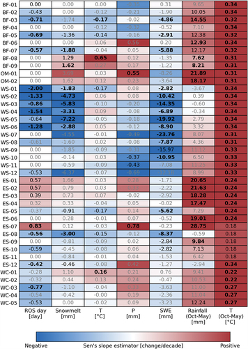
Changes in air temperature and precipitation occurring in individual ROS days were not significant, which indicates that meteorological conditions during ROS days did not change (Fig. 3). This does not correspond to seasonal (October–May) changes in air temperature, where significant increasing trends were detected for all study catchments. This air temperature increase caused the change in precipitation phase resulting in a significant liquid precipitation increase in 17 out of 40 catchments. This shift in precipitation phase towards more rain rather than snowfall may enhance the ROS potential. A strong significant decreasing snowmelt and SWE trends during ROS days were found in multiple catchments, mostly in the Western Sudetes and partially in the Bohemian Forest, both situated in the western parts of the study area.

3.3.2 Monthly and elevation distribution of trends

While the above results obtained at a catchment scale often showed no consistent (although regionally different) trends in ROS days, analysis done for different elevations on a monthly basis enabled a much closer look at the ROS distribution. Figure 4 summarizes trends in ROS days and trends in total rainfall for individual months of the snow season at different elevations (Fig. 4(b) and (d)), together with monthly and elevation distribution of the absolute values for both characteristics (Fig. 4(a) and (c)). Results clearly show that ROS day trends in individual months of the snow season differ across elevation zones. A statistically significant decrease in the number of ROS days during the study period was detected at the end of the snow season in March, at elevations below 700 m a.s.l.; a large decrease was detected at elevations 700–1200 m a.s.l. during April, and a small decrease was detected at elevations above 1200 m a.s.l. in May. The above monthly and elevation-dependent decreases in ROS days were caused by the shortening of the period with existing snow cover on the ground (results not shown) as a response to increasing air temperature, since no corresponding significant changes in rainfall were detected (Fig. 4(d)). The largest decrease in ROS days (Theil-Sen slope equals to −7.3) was detected at elevations of 800–900 m a.s.l. in April, indicating the reduction in number of ROS days by roughly seven days per decade.

Figure 4. (a) Mean number of ROS days, (b) decadal trends in ROS days, (c) mean rainfall and (d) decadal trends in rainfall from October to June at different elevations for the period 1965–2019. The cell values in panels (a) and (c) represent absolute values of ROS days and rainfall, respectively. The cell values in panels (b) and (d) represent Theil-Sen’s slopes of the regression line. Significant Mann-Kendall trends are highlighted in black bold (p < .05) and in black (p < .1), decreasing trends in shades of blue and increasing trends in shades of red (panels B and D). Grey indicates no trends due to no ROS days.

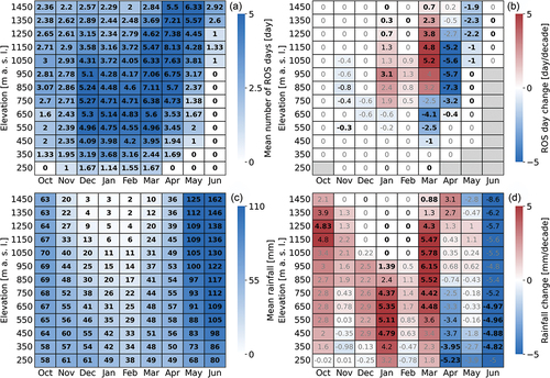
In contrast, a statistically significant increase in ROS days was detected in January at elevations of 900–1000 m a.s.l. An increasing trend was also found at elevations above 1000 m a.s.l. in March, with an increase in the number of ROS days by up to five days per decade. An increase in ROS days found in the middle of the winter season was associated with the fact that more precipitation occurred as rainfall (Fig. 4(d)).

3.4 Hydrological response of ROS events

Using our definition provided in Section 2.3, we identified a total number of 11 852 ROS events at a catchment scale that were analysed for their hydrological response. All ROS events were classified into four groups based on their hydrological response (see Section 2.4). The results showed that 29% (3379 ROS events) caused only negligible runoff (class 1), 43% (5121 ROS events) resulted in low runoff (class 2), 18% (2148 ROS events) caused medium runoff (class 3), and 10% (1204 ROS events) caused high runoff (class 4) (Fig. 5(a)).

Figure 5. (a) Number of ROS events classified according to runoff responses from October to June in the period 1965–2019. (b) Relative contribution of direct ROS event runoff to total monthly direct runoff.

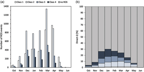
Most of the ROS events, regardless of their runoff class, occurred in March and April, including the most dangerous situations accompanied by high runoffs and enhanced flood risk. Events categorized into classes 2, 3 and 4 were more equally distributed across the main winter season (December–April) compared to class 1 runoff responses.

ROS event runoff (Q_event) contributed 1–30% to the total direct catchment runoff during the individual months of the snow season, with the largest ROS event contribution in January. Classes 3 and 4 were the main contributors from November to February (4–12%), and class 2 was the main contributor from March to the end of the snow season (3–9%) (Fig. 5(b)). ROS event runoff contributed 3–32% to the total direct runoff within individual study catchments, with a mean ROS event contribution of 17% (results not shown).

Calculation of ROS event runoff volumes enabled us to assess their changes over time (Fig. 6). Results showed that the statistically significant decreases in ROS event runoff volumes were detected only for classes 2 and 3 in April, which can be explained by an overall decrease in snow storage (result not shown). Other identified trends are rather weak and not significant, although a certain increase in runoff volumes was detected particularly for classes 2 and 3 for January to March and for the most extreme class 4 in March.

Figure 6. Trends in runoff volume classes of ROS events (Qevent) during the period 1965–2019. The cell values represent Theil-Sen’s slopes of the regression line. Significant Mann-Kendall trends are highlighted in black bold (p < .05) and in black (p < .1), decreasing trends in shades of blue and increasing trends in shades of red.

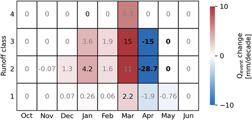
The analysis of trends in ROS event runoff volume was also carried out for individual catchments. However, detected trends were rather weak and no regional dependencies were found (results not shown). A statistically significant increase in runoff volume was detected only in six catchments (out of 40) in March, and a significant volume decrease was found in eight catchments in April.

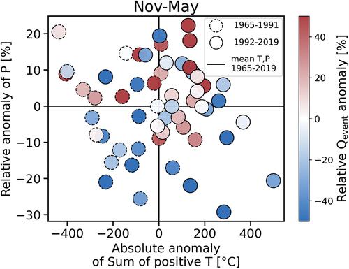
Besides trends in ROS event runoff responses, an interesting question is also how inter-annual changes in driving climatic variables control the annual volume of ROS event runoff. To answer this question, annual anomalies in two key ROS drivers – the seasonal sum of positive air temperature and seasonal precipitation – were related to anomalies in ROS event runoff volume in individual years (Fig. 7). Results expectedly showed that the largest ROS event runoff volume anomalies occurred in both wet and warm years (top right quadrant in Fig. 7), although seasonal precipitation seems to be more important. An increasing number of years with positive anomalies in the sum of positive air temperatures occurring in the second half of the study period (1992–2019; solid circle margins in Fig. 7) did not lead to more positive anomalies of ROS runoff volumes in this period compared to the first half of the study period. This partial result corresponds to mostly missing trends in ROS runoff volumes in individual catchments, as described above.

Figure 7. Relationship between relative anomaly in November to May precipitation (y-axis), absolute anomaly in November to May sum of positive air temperatures (x-axis), and relative anomaly in ROS event runoff volume (colour scale) in two different periods, 1965–1991 and 1992–2019.

4 Discussion

4.1 Uncertainty in modelling approach

In this study, we used a semi-distributed hydrological model to derive individual components of the rainfall–runoff process and to assess the occurrence and selected characteristics of ROS, similar to Freudiger et al. (2014) who assessed ROS frequencies of ROS events in Germany. Our modelling approach may raise questions related to model parameterization and structure, specifically how individual model parameters and procedures represent real natural processes, such as ROS events. The uncertainty arising from the model parameterization needs to be addressed, since the results presented are based on runoff simulations, and primarily on modelled SWE, as one of the parameters that defines ROS occurrence in this study. The HBV model was calibrated automatically against both SWE and observed runoff. Calibration results were evaluated using a combination of three objective functions (see Section 2.2) originally for study by Jenicek and Ledvinka (2020) and further used by Nedelcev and Jenicek (2021) and Sipek et al. (2021). One hundred calibration runs were performed to lower the overall parameter uncertainty, and multi-criteria model calibration enabled us to better control the simulation of the SWE in individual catchments. ROS analyses were performed at a multi-catchment level, using input data from climate stations limited to air temperature and precipitation data, which did not allow the use of the energy balance approach. Therefore, we used the modified degree-day approach implemented in the HBV model. While we are aware of the limitations of bucket-type approaches in general and the degree-day approach specifically, model intercomparisons in the literature have demonstrated repeatedly that simple model approaches can provide results at least as good as those produced by more complex, physically-based models in practice, despite the latter being superior in theory (Seibert and Bergström 2022). Despite the limitations of degree-day approaches, several studies proved to be sufficient for simulating snow storage at a catchment scale under climate change (Addor et al. 2014, Etter et al. 2017, Jenicek et al. 2021) or even ROS runoff (Freudiger et al. 2014, Juras et al. 2021). This is especially the case for the variation of the degree-day approach we are using because it also accounts for liquid water content stored in the snow and refreezing. Additionally, the recent study by Girons Lopez et al. (2020) largely confirmed that the current HBV snow routine provides results at a catchment scale that are hard to improve despite increasing physical realism.

Since the air temperature and precipitation data were adjusted for individual elevation zones using lapse rates calibrated separately for each catchment, we assume a high level of accuracy to correctly define ROS and non-ROS days, related trends and hydrological responses related to ROS. This was recently shown by Nedelcev and Jenicek (2021), who tested long-term trends in simulated and observed seasonal precipitation, air temperature and SWE in the same study domain and found no major differences.

Model calibration showed mostly satisfactory results (Fig. S1), with Nash-Sutcliffe efficiency values higher than 0.7. For example, Moriasi et al. (2015) argued that Nash-Sutcliffe efficiency values above 0.5 using the daily time step can be regarded as a satisfactory modelling result. Nevertheless, it might be difficult to agree on specific efficiency benchmarks, or on how to define the lower benchmark for good model performance (Seibert et al. 2018). Thus, model justification required further model testing, presented in the Supplementary material (Figs S2–S5).

We assessed how 100 model parameterizations resulting in 100 simulations for each catchment impacted the variability of the investigated parameters, such as the number of ROS days (Fig. S2). Results showed that simulated numbers of ROS days do not vary significantly in five selected catchments, except one in the Western Carpathians (WC-04). Nevertheless, results showed that median simulations resulted also in close-to-median numbers of ROS days, which reduces the sensitivity of our results to individual model parameterizations and thus increases the overall reliability of the model.

Since the number of stations with long-term monitoring of SWE was limited, we used only 15 stations with weekly SWE observations. Because of the shorter time series and weekly data, we obtained a reduced number of cases, which were compared with simulated ROS days from the same elevation zone as observed data (Figs S3 and S4). However, the potential disagreement of the modelled values with observed ones does not necessarily mean that the model is incorrect. Observed data are also uncertain, especially due to the representativeness (or lack thereof) of the measurement location (wind influence, forest effects, slope orientation etc.). Some of the study catchments are relatively larger than others and more diverse and cannot be represented by one SWE time series. Furthermore, the quality of SWE measurements performed by observers decreases back in time.

The comparison of observed and simulated ROS days showed that the simulated number of ROS days was often lower than the observed one (Fig. S4). This was probably due to inaccuracies in simulated SWE at the end of the snow season caused by overestimation of simulated snowmelt rates resulting in earlier snowmelt and thus a lower number of simulated ROS days. Additionally, 27% of ROS events were overestimated in terms of hydrological response, although 54% of all ROS events were assigned to the same runoff class based on simulated and observed data (Fig. S5).

Although the model and observed values partly differ in absolute terms, we did not find any major inconsistencies in model simulations. Since our analysis was focused mainly on the relative differences and trends in ROS days and ROS events rather than on absolute values, we believe that the model provided sufficiently good simulations. More detailed testing of SWE simulations was carried out by Jenicek et al. (2021) and Nedelcev and Jenicek (2021), who worked with the same set of catchments as used in our study. Therefore, we refer readers to those studies for further information.

4.2 ROS definition

Defining ROS situations by several selection criteria that are dependent on threshold values may appear arbitrary, since changes in these threshold values can affect the absolute number of identified ROS days and ROS events. Nevertheless, based on the literature review, there is no consistent definition for either an ROS day or an ROS event, which limits the comparison of results across different studies (Brandt et al. 2022).

In our study, selection criteria that correspond to previous studies were used; a daily mean air temperature of 0°C to separate snow and rain was also used by Surfleet and Tullos (2013), Bieniek et al. (2018), and Crawford et al. (2020); an SWE threshold of 10 mm was used by Freudiger et al. (2014), Trubilowicz and Moore (2017) and Huang et al. (2022); and a daily rainfall intensity threshold of 5 mm was applied by Trubilowicz and Moore (2017) and Pall et al. (2019). The air temperature threshold value is apparently the most important criterion because it controls precipitation phase. Definition of the threshold temperature might be difficult using daily data, especially for days with air temperature near the freezing point, or during days with high daily temperature amplitude (cold nights and warmer days in spring) resulting in a mean daily temperature around zero despite the fact that precipitation phase may change during day. Thus, the total number of analysed ROS days and ROS events may differ.

However, the threshold value of 0°C used in this study agrees with the findings of Jennings et al. (2018), who argued that air temperature at which rain and snow fall in equal frequency ranges from −0.4 to 2.4°C for 95% of the stations across the Northern Hemisphere. Threshold temperature was one of the calibrated parameters in the HBV model. Based on our results, the mean threshold temperature reached −0.4°C for the study catchments. However, using calibrated values might be inappropriate since they may compensate for other processes or imperfect model structure (precipitation undercatch, temperature or precipitation lapse rates, SWE measurements etc.). Therefore, we decided to use one value for all catchments that is close to the mean of calibrated threshold temperature values. Although we are aware that the threshold value influences the absolute number of ROS days/events, our study rather assessed trends and inter-annual differences, which are less sensitive in terms of the absolute number of events.

Thresholds for rain and SWE seem to be less sensitive. A sensitivity analysis in our previous study performed partly at the same study area revealed that ROS characteristics remain similar when different limits for SWE and minimum rainfall were applied (Juras et al. 2021). In addition, threshold parameters for SWE and precipitation may also differ spatially, since snow cover is distributed unevenly and rainfall intensity is usually not constant.

4.3 ROS occurrence

The temporal and spatial distribution of ROS during the winter season is controlled by weather conditions. Accordingly, research studies focusing on ROS are usually area specific (Li et al. 2019). Results showed some regional differences in analysed parameters (Fig. 3, Table S1). Despite the relative proximity of the studied regions, climate variables (air temperature, precipitation, snow parameters) affecting ROS occurrence differed considerably during the cold season, probably in relation to increasing continentality from west to east.

In general, ROS occurrence depends on snowpack existence and rainfall occurrence. In the study area, the typical ROS season occurred from November to May (with rather rare events in October and June at the highest elevations), which is in good agreement with findings by Freudiger et al. (2014), who analysed ROS events in catchments located in Germany.

We identified a total of 15 894 ROS days in all 40 catchments during the study period, 1965–2019. We found a typical ROS day to be a day with daily mean air temperature ranging from 1.5°C at the lowest elevations to 2.9°C at the highest elevations (Fig. 2). These values as well as typical rainfall intensities and SWEs do not differ from those reported in other European regions with similar climate (Garvelmann et al. 2015, Würzer et al. 2016, Trubilowicz and Moore 2017). However, comparison of ROS situations across different regions and studies may be difficult, since ROS characteristics are often determined differently across studies and in different temporal resolutions.

Our results showed that air temperature, total rainfall, SWE, and snowmelt during ROS days increased with elevation. The higher mean air temperature and rainfall amount typical for ROS days at higher elevations may be explained by the fact that most of the ROS occurred in the spring months (even into May and June), with overall higher air temperatures leading to more water vapor in the atmosphere and thus more intensive rainfall compared to winter. Another reason for this elevation dependence might be that ROS days at the highest elevations are usually associated with more intense warm air mass advection typical for low pressures, which brings more intensive rainfall followed by rapid snowmelt, while ROS situations are often distributed throughout the winter season at lower elevations where air temperature often fluctuated around 0°C.

Several studies pointed out that the initial properties of snowpack and its retention capacity are both important factors with a strong influence on runoff formation during ROS (Garvelmann et al. 2015, Würzer et al. 2016). As a result, not all ROS events generated runoff increase (Merz and Blöschl 2003, Wayand et al. 2015, Juras et al. 2021). We identified 10% of all ROS events that caused high runoff (according to defined runoff classes), and most of the ROS events (72%) did not cause any significant runoff increase (low or negligible runoff). Our results are consistent with Juras et al. (2021) in this respect, who used a similar runoff type classification analysed in a partly overlapping study area.

Most of the negligible- and low-runoff ROS events occurred in March and April, probably due to relatively high snow storage which stores a lot of liquid water coming from rainfall. Dangerous high-runoff situations occurred mainly in March, probably due to more intensive spring rainfall, generally higher air temperature, and high SWE which was often at its seasonal maximum, resulting in faster snowmelt. Earlier medium and high runoff responses during winter season (December–February) might be influenced by the non-ripe snowpack with lower snow densities and prevailing preferential flow paths that allowed rainwater to efficiently propagate through the snowpack, resulting in a faster and higher runoff (Juras et al. 2017).

4.4 ROS trends

At a catchment scale, Mann-Kendall trend tests showed a statistically significant change (p value < .1) in ROS days in 21 out of 40 catchments. However, the identified trends are rather weak and not consistent across catchments, although some regional patterns can be identified. Opposite trends in numbers of ROS days were detected in the Eastern Sudetes (increasing trends) and Western Sudetes (decreasing trends), despite their proximity (150 km). We hypothesize that these opposite trends are caused by different synoptic situations that influence precipitation amount and its spatial distribution in individual mountain ranges (Juras et al. 2021). For instance, catchments in the Western Sudetes experience high annual precipitation (above 1000 mm) that leads to relatively more ROS days compared to the Eastern Sudetes (results not shown). In contrast, rapid shortening of the period with snow on the ground in the Western Sudetes investigated by Nedelcev and Jenicek (2021) causes ultimately decreasing trends in the number of ROS days.

In general, our results showed that significant change in ROS days related to increasing air temperature is not clear at a catchment scale. Since both elevation and air temperature are important ROS drivers, there is an ROS decrease due to the shortening of the period with existing snow cover on the ground on the one hand, while there is an increase due to a decrease in snowfall fraction on the other hand. Trends showing elevation-dependent changes and monthly changes are more pronounced and consistent with results of other studies (Li et al. 2019, López-Moreno et al. 2021), even with those that focus on ROS projections for the future (Sezen et al. 2020).

Results clearly showed that ROS trends in individual months of the winter season differ across elevations. We detected a significant ROS decrease at elevations below 700 m a.s.l. (mainly in March) and at elevations from 700 to 1200 m a.s.l. (mainly in April), which supports the findings of Surfleet and Tullos (2013), Musselman et al. (2018), and Li et al. (2019). In contrast, a predicted increase in the number of ROS days at higher elevations, presented by Il Jeong and Sushama (2017), Trubilowicz and Moore (2017), and Li et al. (2019), cannot be suggested uniformly throughout the snow season since trends differ across individual months. At higher elevations, we found a significant ROS decrease in late winter (May) associated with the shorter period with snow cover on the ground, which is in good agreement with the study by Sezen et al. (2020). A significant ROS increase was detected only in the middle of the snow season (January and March) since more precipitation occurred as rain rather than snow, as also recently found by Nedelcev and Jenicek (2021) for the same study area. The main reason for these differences in ROS patterns at higher elevations is that different definitions of ‘high elevation’ were used across the studies. Beniston and Stoffel (2016) showed that the temperature increase observed in Switzerland in the period 1960–2015 has contributed directly to the increase in the number of ROS events by about 40% at low elevations (below 1500 m a.s.l.). This seems to fit well with our results for elevations above 1000 m a.s.l. The offset of roughly 500 m might be caused by the more northern latitude of our study area and its partly different climate.

5 Conclusion

We evaluated the frequency and ongoing trends in ROS days and their runoff responses at different elevations. We were particularly focused on lower elevation mountain ranges since they represent rain–snow transition areas with large changes in snow storage affecting ROS occurrence. Based on the results, we can draw the following conclusions.

We identified a total of 15 894 ROS days at a catchment scale in the period 1965–2019. Mean snowmelt during the ROS days reached 9 mm and the mean SWE was 111 mm. Both parameters showed strong, significant decreasing trends in multiple catchments. Typical mean air temperature during the ROS days was 2°C and mean daily precipitation reached 12 mm. Generally, values of all four variables increased with elevation.

The results showed a statistically significant change in the number of ROS days in multiple catchments. However, these changes were rather small and not consistent at a catchment scale. In contrast, strong, significant trends in ROS days were identified for specific months at different elevations. The largest decrease was detected at elevations from 700 to 1200 m a.s.l. during April, most likely caused by a shortening of the period with existing snow cover on the ground due to increasing air temperature. The largest increase was detected at elevations above 1000 m a.s.l. in March, which was associated with more frequent rainfall due to the increasing air temperature.

We identified a total of 11 852 ROS events at a catchment scale. About 10% of all ROS events have flood-generation potential (they were classified as high-runoff events) and these events occurred mostly in March.

ROS event runoff contributed 3–32% to the total direct catchment runoff during the snow season, with the largest relative contribution in January. The changes in ROS event runoff volume were mostly weak and not consistent across individual catchments. The largest relative ROS runoff volume anomaly resulted from the combination of a positive anomaly in the sum of positive air temperatures and a positive anomaly in the seasonal precipitation, where the latter seems to be of greater importance.

The results showed that changes in ROS days and their runoff responses differ among individual study catchments, across elevations and for different months during the snow season. Additionally, the impact of increasing air temperature and thus partly decreasing snow storage and shorter snow cover duration clearly affected the ROS spatial and temporal distribution. Overall, our findings contribute to a better understanding of factors leading to ROS events and their runoff responses related to climate variability and projected future climate changes.

Acknowledgements

Many thanks are due to Tracy Ewen for improving the language. We also thank associate editor Stephanie Kampf, reviewer Juraj Parajka and one anonymous reviewer for their valuable feedback.

Disclosure statement

No potential conflict of interest was reported by the authors.

Data availability statement

The data that support the findings of this study are available from the corresponding author, OH, upon reasonable request.

Supplementary material

Supplemental data for this article can be accessed online at https://doi.org/10.1080/02626667.2023.2177544

Additional information

Funding

This work was supported by the Charles University Grant Agency, project no. GAUK 272119 (Modelling of future effects of changes in snow storages on occurrence and extremity of runoff caused by rain-on-snow events) and Technology Agency of the Czech Republic (project SS02030040).

References

- Addor, N., et al., 2014. Robust changes and sources of uncertainty in the projected hydrological regimes of Swiss catchments. Water Resources Research, 50 (10), 7541–7562. doi:10.1002/2014WR015549
- Beniston, M. and Stoffel, M., 2016. Rain-on-snow events, floods and climate change in the Alps: events may increase with warming up to 4 °C and decrease thereafter. Science of the Total Environment, 571, 228–236. doi:10.1016/j.scitotenv.2016.07.146
- Bieniek, P.A., et al., 2018. Assessment of Alaska rain-on-snow events using dynamical downscaling. Journal of Applied Meteorology and Climatology, 57 (8), 1847–1863. doi:10.1175/JAMC-D-17-0276.1
- Blahusiakova, A., et al., 2020. Snow and climate trends and their impact on seasonal runoff and hydrological drought types in selected mountain catchments in Central Europe. Hydrological Sciences Journal, 65 (12), 2083–2096. doi:10.1080/02626667.2020.1784900
- Blöschl, G., et al., 2019. Twenty-three unsolved problems in hydrology (UPH)–a community perspective. Hydrological Sciences Journal, 64 (10), 1141–1158. doi:10.1080/02626667.2019.1620507
- Brandt, W.T., et al., 2022. A review of the hydrologic response mechanisms during mountain rain-on-snow. Frontiers in Earth Science, 10, 791760. doi:10.3389/feart.2022.791760
- Brunner, M.I., et al., 2019. Future shifts in extreme flow regimes in Alpine regions. Hydrology and Earth System Sciences, 23 (11), 4471–4489. doi:10.5194/hess-23-4471-2019
- Cohen, J., Ye, H., and Jones, J., 2015. Trends and variability in rain-on-snow events. Geophysical Research Letters, 42 (17), 7115–7122. doi:10.1002/2015GL065320
- Crawford, A.D., et al., 2020. Synoptic climatology of rain-on-snow events in Alaska. Monthly Weather Review, 148 (3), 1275–1295. doi:10.1175/MWR-D-19-0311.1
- Etter, S., et al., 2017. Climate change impacts on future snow, ice and rain runoff in a Swiss mountain catchment using multi-dataset calibration. Journal of Hydrology: Regional Studies, 13, 222–239.
- Freudiger, D., et al., 2014. Large-scale analysis of changing frequencies of rain-on-snow events with flood-generation potential. Hydrology and Earth System Sciences, 18 (7), 2695–2709. doi:10.5194/hess-18-2695-2014
- Garvelmann, J., Pohl, S., and Weiler, M., 2014. Variability of observed energy fluxes during rain-on-snow and clear sky snowmelt in a midlatitude mountain environment. Journal of Hydrometeorology, 15 (3), 1220–1237. doi:10.1175/JHM-D-13-0187.1
- Garvelmann, J., Pohl, S., and Weiler, M., 2015. Spatio-temporal controls of snowmelt and runoff generation during rain-on-snow events in a mid-latitude mountain catchment. Hydrological Processes, 29 (17), 3649–3664. doi:10.1002/hyp.10460
- Girons Lopez, M., et al., 2020. Assessing the degree of detail of temperature-based snow routines for runoff modelling in mountainous areas in central Europe. Hydrology and Earth System Sciences, 24 (9), 4441–4461. doi:10.5194/hess-24-4441-2020
- Hammond, J.C., Saavedra, F.A., and Kampf, S.K., 2018. How does snow persistence relate to annual streamflow in mountain watersheds of the western U.S. with wet maritime and dry continental climates? Water Resources Research, 54 (4), 2605–2623. doi:10.1002/2017WR021899
- Hotovy, O. and Jenicek, M., 2020. The impact of changing subcanopy radiation on snowmelt in a disturbed coniferous forest. Hydrological Processes, 34 (26), 5298–5314. doi:10.1002/hyp.13936
- Huang, H., et al., 2022. Changes in mechanisms and characteristics of western U.S. floods over the last sixty years. Geophysical Research Letters.
- Il Jeong, D. and Sushama, L., 2017. Rain-on-snow events over North America based on two Canadian regional climate models. Climate Dynamics, 50 (1–2), 303–316. doi:10.1007/s00382-017-3609-x
- Jenicek, M., et al., 2021. Future changes in snowpack will impact seasonal runoff and low flows in Czechia. Journal of Hydrology: Regional Studies, 37, 100899.
- Jenicek, M. and Ledvinka, O., 2020. Importance of snowmelt contribution to seasonal runoff and summer low flows in Czechia. Hydrology and Earth System Sciences, 24 (7), 3475–3491. doi:10.5194/hess-24-3475-2020
- Jennings, K.S., et al., 2018. Spatial variation of the rain-snow temperature threshold across the Northern Hemisphere. Nature Communications, 9 (1), 1–9. doi:10.1038/s41467-018-03629-7
- Jennings, K. and Jones, J.A., 2015. Precipitation-snowmelt timing and snowmelt augmentation of large peak flow events, western Cascades, Oregon. Water Resources Research, 51 (9), 7649–7661. doi:10.1002/2014WR016877
- Juras, R., et al., 2017. Rainwater propagation through snowpack during rain-on-snow sprinkling experiments under different snow conditions. Hydrology and Earth System Sciences, 21 (9), 4973–4987. doi:10.5194/hess-21-4973-2017
- Juras, R., et al., 2021. What affects the hydrological response of rain-on-snow events in low-altitude mountain ranges in Central Europe? Journal of Hydrology, 603, 127002. doi:10.1016/j.jhydrol.2021.127002
- Kendall, M.G., 1975. Rank correlation measures. London: Charles Griffin.
- Krug, A., et al., 2020. On the temporal variability of widespread rain-on-snow floods. Meteorologische Zeitschrift, 29 (2), 147–163. doi:10.1127/metz/2020/0989
- Li, D., et al., 2019. The role of rain-on-snow in flooding over the conterminous United States. Water Resources Research, 55 (11), 8492–8513. doi:10.1029/2019WR024950
- Li, Z., et al., 2020. Declining snowfall fraction in the alpine regions, Central Asia. Scientific Reports, 10 (1), 1–12. doi:10.1038/s41598-019-56847-4
- Lindström, G., et al., 1997. Development and test of the distributed HBV-96 hydrological model. Journal of Hydrology, 201 (1–4), 272–288. doi:10.1016/S0022-1694(97)00041-3
- López-Moreno, I., et al., 2021. Changes in the frequency of global high mountain rain-on-snow events due to climate warming. Environmental Research Letters.
- Mann, H.B., 1945. Nonparametric tests against trend. Econometrica, 13 (3), 245. doi:10.2307/1907187
- Marks, D., et al., 1998. The sensitivity of snowmelt processes to climate conditions and forest cover during rain-on-snow: a case study of the 1996 Pacific Northwest flood. Hydrological Processes, 12 (10–11), 1569–1587. doi:10.1002/(SICI)1099-1085(199808/09)12:10/11<1569::AID-HYP682>3.0.CO;2-L
- Marty, C., et al., 2017. How much can we save? Impact of different emission scenarios on future snow cover in the Alps. Cryosphere, 11 (1), 517–529. doi:10.5194/tc-11-517-2017
- Mazurkiewicz, A.B., Callery, D.G., and McDonnell, J.J., 2008. Assessing the controls of the snow energy balance and water available for runoff in a rain-on-snow environment. Journal of Hydrology, 354 (1–4), 1–14. doi:10.1016/j.jhydrol.2007.12.027
- Mccabe, G.J., Clark, M.P., and Hay, L.E., 2007. Rain-on-snow events in the western United States. American Meteorological Society, 88 (3), 319–328. doi:10.1175/BAMS-88-3-319
- Merz, R. and Blöschl, G., 2003. A process typology of regional floods. Water Resources Research, 39 (12), 1340. doi:10.1029/2002WR001952
- Moriasi, D.N., et al., 2015. Hydrologic and water quality models: performance measures and evaluation criteria. Transactions of the ASABE, 58 (6), 1763–1785.
- Musselman, K.N., et al., 2018. Projected increases and shifts in rain-on-snow flood risk over western North America. Nature Climate Change.
- Nash, J.E. and Sutcliffe, J.V., 1970. River flow forecasting through conceptual models part I - A discussion of principles. Journal of Hydrology, 10 (3), 282–290. doi:10.1016/0022-1694(70)90255-6
- Nedelcev, O. and Jenicek, M., 2021. Trends in seasonal snowpack and their relation to climate variables in mountain catchments in Czechia. Hydrological Sciences Journal, 66 (16), 2340–2356. doi:10.1080/02626667.2021.1990298
- Notarnicola, C., 2020. Hotspots of snow cover changes in global mountain regions over 2000–2018. Remote Sensing of Environment, 243, 111781. doi:10.1016/j.rse.2020.111781
- Ohba, M. and Kawase, H., 2020. Rain-on-snow events in Japan as projected by a large ensemble of regional climate simulations. Climate Dynamics, 55 (9–10), 2785–2800. doi:10.1007/s00382-020-05419-8
- Oudin, L., et al., 2005. Which potential evapotranspiration input for a lumped rainfall-runoff model? Part 2 - towards a simple and efficient potential evapotranspiration model for rainfall-runoff modelling. Journal of Hydrology, 303 (1–4), 290–306. doi:10.1016/j.jhydrol.2004.08.026
- Pall, P., Tallaksen, L.M., and Stordal, F., 2019. A climatology of rain-on-snow events for Norway. Journal of Climate, 32 (20), 6995–7016. doi:10.1175/JCLI-D-18-0529.1
- Pradhanang, S.M., et al., 2013. Rain-on-snow runoff events in New York. Hydrological Processes, 27 (21), 3035–3049. doi:10.1002/hyp.9864
- Rennert, K.J., et al., 2009. Soil thermal and ecological impacts of rain on snow events in the circumpolar Arctic. Journal of Climate, 22 (9), 2302–2315. doi:10.1175/2008JCLI2117.1
- Seibert, J., 2000. Multi-criteria calibration of a conceptual runoff model using a genetic algorithm. Hydrology and Earth System Sciences, 4 (2), 215–224. doi:10.5194/hess-4-215-2000
- Seibert, J., et al., 2018. Upper and lower benchmarks in hydrological modelling. Hydrological Processes, 32 (8), 1120–1125. doi:10.1002/hyp.11476
- Seibert, J. and Bergström, S., 2022. A retrospective on hydrological catchment modelling based on half a century with the HBV model. Hydrology and Earth System Sciences, 26 (5), 1371–1388. doi:10.5194/hess-26-1371-2022
- Seibert, J. and Vis, M.J.P., 2012. Teaching hydrological modeling with a user-friendly catchment-runoff-model software package. Hydrology and Earth System Sciences, 16 (9), 3315–3325. doi:10.5194/hess-16-3315-2012
- Sen, P.K., 1968. Estimates of the regression coefficient based on Kendall’s tau. Journal of the American Statistical Association, 63 (324), 1379–1389. doi:10.1080/01621459.1968.10480934
- Serquet, G., et al., 2011. Seasonal trends and temperature dependence of the snowfall/precipitation- day ratio in Switzerland. Geophysical Research Letters, 38 (7), L07703. doi:10.1029/2011GL046976
- Sezen, C., et al., 2020. Investigation of rain-on-snow floods under climate change. Applied Sciences (Switzerland), 10, 4.
- Sipek, V., et al., 2021. Catchment storage and its influence on summer low flows in central European mountainous catchments. Water Resources Management, 35 (9), 2829–2843. doi:10.1007/s11269-021-02871-x
- Surfleet, C.G. and Tullos, D., 2013. Variability in effect of climate change on rain-on-snow peak flow events in a temperate climate. Journal of Hydrology, 479, 24–34. doi:10.1016/j.jhydrol.2012.11.021
- Trubilowicz, J.W. and Moore, R.D., 2017. Quantifying the role of the snowpack in generating water available for run-off during rain-on-snow events from snow pillow records. Hydrological Processes, 31 (23), 4136–4150. doi:10.1002/hyp.11310
- Vlach, V., Ledvinka, O., and Matouskova, M., 2020. Changing low flow and streamflow drought seasonality in central European headwaters. Water, 12 (12), 3575. doi:10.3390/w12123575
- Wayand, N.E., Lundquist, J.D., and Clark, M.P., 2015. Modeling the influence of hypsometry, vegetation, and storm energy on snowmelt contributions to basins during rain-on-snow floods. Water Resources Research, 51 (10), 8551–8569. doi:10.1002/2014WR016576
- Wever, N., et al., 2016. Simulating ice layer formation under the presence of preferential flow in layered snowpacks. Cryosphere, 10 (6), 2731–2744. doi:10.5194/tc-10-2731-2016
- Würzer, S., et al., 2016. Influence of initial snowpack properties on runoff formation during rain-on-snow events. Journal of Hydrometeorology, 17 (6), 1801–1815. doi:10.1175/JHM-D-15-0181.1
- Würzer, S., et al., 2017. Modelling liquid water transport in snow under rain-on-snow conditions - Considering preferential flow. Hydrology and Earth System Sciences, 21 (3), 1741–1756. doi:10.5194/hess-21-1741-2017
- Würzer, S. and Jonas, T., 2018. Spatio-temporal aspects of snowpack runoff formation during rain on snow. Hydrological Processes, 32 (23), 3434–3445. doi:10.1002/hyp.13240