Proglacial streams runoff dynamics in Devil´s Bay, Vega Island, Antarctica

ABSTRACT

Increasing temperatures in Antarctica have resulted in the enlargement of proglacial regions on the Antarctic Peninsula, following glacier melt. This melt has increased river activity yet direct runoff measurements remain scarce in Antarctica, despite it acting as a proxy for glacial ablation. Here, we present discharge and water temperature data from 2013 for three streams on Vega Island and discuss their relationship with air temperature. The average discharge at the largest stream was 0.523 m³s⁻¹ with a maximum of 5.510 m³s⁻¹ – among the highest recorded in Antarctica. The rivers continued to flow even when temperatures dropped to −7°C, indicating that a large proportion of the total runoff originated sub-glacially. This is supported by the one-day time lag between air and water temperatures. Using river discharge as a proxy, we measured 124.5 ± 14.4 mm w.e. of ablation. This indirect measurement proved an effective tool to complement classic glaciological observations.

KEYWORDS:

• runoff
• water temperature
• glaciers
• eastern Antarctic Peninsula
• atmospheric conditions

Editor A. Fiori Associate Editor (not assigned)

1 Introduction

The Antarctic Peninsula region experienced rapid environmental changes during the 20^th century, which have been associated with increases in the air temperature observed over the same period (Turner et al. 2016). As highlighted by Gonzales and Fortuny (2018) and Oliva et al. (2017), changes in air temperature are spatially discontinuous, and the northeastern sector of the Antarctic Peninsula has seen some of the largest increases. This spatial variability can be more acutely seen in precipitation trends (Turner et al. 2019), with drying observed in East Antarctica (Robinson et al. 2018) and increased snowfall observed over the Antarctic Ice Sheet (Medley and Thomas 2019). Atmospheric conditions vary not only spatially, but also temporally; rainfall events in the Antarctic Peninsula region decreased between 1998 and 2015, but are projected to increase in frequency and intensity in the future (Vignon et al. 2021). This spatial and temporal variability is of significant relevance when looking at the changes in river dynamics, including discharge and sediment transport. In turn, changes in river and sediment dynamics can have a profound effect on the biodiversity of freshwater (Foreman et al. 2004, García-Rodríguez et al. 2021) and marine ecosystems (Sahade et al. 2015, Hodson et al. 2017). Similarly, water temperature, including its variability and long-term changes, is also crucial for maintaining living organisms (Brown et al. 2005, Johnson et al. 2014). The relationship between water temperature and freshwater organisms is often studied in Arctic or sub-Arctic Canadian catchments (e.g. Daigle et al. 2015, Padilla et al. 2015). A good example of this process in Antarctica is the re-appearance of the fairy shrimp (Branchinecta gaini) in the lakes of James Ross Island, where it was abundant during a significant period of Holocene (Björck et al. 1996) but re-appeared only recently because of the extension of an ice-free period on the studied lakes (Nedbalová et al. 2017). Additionally, water temperature and its dynamics concerning ongoing climate change are important globally (Du et al. 2022) and have been highlighted in polar regions (e.g. for Greenland in Docherty et al. 2019).

Glacierized catchments are affected by accelerated glacier mass loss worldwide (Hugonnet et al. 2021), with certain regions already experiencing a decline in meltwater runoff since the glaciers have passed the point of maximum melt (Huss and Hock 2018). Therefore, it is essential to gather information on the behaviour of hydrological systems related to glacial environments that are likely to be affected by ongoing environmental changes (e.g. Young et al. 2021). Despite this need, studies on fluvial systems are relatively scarce in Antarctica and are often concentrated in a few major deglaciated areas. More complex studies of the runoff regime and its impact on transporting minerals and sediments are even scarcer in the Antarctic region. Runoff dynamics were studied on James Ross Island (Kavan et al. 2017, Kavan 2022), in the Maritime Antarctica region (e.g. Inbar 1995, Szilo and Bialik 2017, Stott and Convey 2021), and as a part of more complex research projects in the McMurdo Dry Valleys (Shaw and Healy 1980, Hawke and McConchie 2001). The runoff regime of glacierized catchments and its relationship to atmospheric parameters is frequently studied in regions where it affects the availability of water resources for agriculture, industry or drinking water supply (e.g. Krysanova et al. 2015, Shijin et al. 2021, Motschmann et al. 2022). However, little is known about those in Antarctica, where the impact of human activities is minimal.

Long-term studies on runoff production and the transport of nutrients are primarily available from the McMurdo Dry Valleys (e.g. Welch et al. 2010, Olund et al. 2018, Harmon et al. 2021). Fountain et al. (2004) emphasized the importance of cryoconite holes in generating runoff from glaciers and reported that at least 13% of the observed glacier runoff originated in the subsurface hydrological network formed by interconnected cryoconites on glaciers. Melting of the glacier surface was identified as an important component in the overall runoff production in this relatively cold region (e.g. Johnston et al. 2005, Bergstrom et al. 2021). Apart from its direct impacts on the surrounding deglaciated areas, runoff generated within the glacier system also affects the behaviour of the glacier itself, including the velocity of the glacier flow (e.g. Chu 2014). The hydrological regime in the Antarctic Peninsula region is often driven by more variable meltwater sources such as glacier melt (Stott and Convey 2021), seasonal snow cover or permafrost thawing (e.g. Kavan et al. 2017) or liquid precipitation in Maritime Antarctica (e.g. Szilo and Bialik 2017). The spatial and temporal variability of runoff in polar regions is driven mainly by surface air temperature, solar radiation, precipitation and snow cover (e.g. Li et al. 2010, Nowak and Hodson 2013, Lehmann-Konera et al. 2019). Surface air temperatures are usually considered to be the most important factor in the glacierized catchments of Alpine mountains (e.g. Schmieder et al. 2016), Maritime Antarctica (e.g. Falk et al. 2018) and most of the Arctic (e.g. Nowak and Hodson 2013). In contrast, solar radiation is the main driver of melt in extremely cold environments, such as the McMurdo Dry Valleys (McConchie et al. 1990).

In this study, we assess the intra-seasonal runoff dynamics of three glacier-fed streams on Vega Island, eastern Antarctic Peninsula. We also investigate the relationship between air temperature and river discharge and look at the effects of runoff from the adjacent glaciers. Additionally, we aim to establish runoff as a proxy to estimate the summer ablation of the Glaciar Bahía del Diablo (GBD) as a useful complementary technique to classical glaciological observations. Moreover, direct discharge observations in Antarctica are rather rare, thus our contribution can enhance our knowledge of the behaviour of these freshwater geosystems.

1.1 Study site

Our study focuses on the northern part of Vega Island, often referred to as “Devil’s Bay,” in the James Ross Archipelago located to the northeast of the Antarctic Peninsula (Fig. 1). Vast dome glaciers located on the volcanic mesas (around 220 m a.s.l.) surround the ice-free area of about 12 km². These dome glaciers have several outlet glaciers, including the GBD in our study area (Marinsek and Ermolin 2015) i.e. Devil’s Bay glacier. The climate of Vega Island is cold semi-arid, with a mean annual air temperature, measured at the nearby J.G. Mendel Station (on northern James Ross Island, ~25 km to the west, altitude 10 m a.s.l.), of −7.0°C (2006–2015) with summer daily maxima exceeding +10°C and winter minima dropping below −30°C (Hrbáček et al. 2017). The whole James Ross Archipelago lies in the precipitation shadow of the Antarctic Peninsula, with annual precipitation estimates of 300–500 mm of water equivalent (w.e.) by van Lipzig et al. (2004) or even up to 700 mm w.e.year⁻¹ by van Wessem et al. (2016). The combination of low precipitation and increasing air temperatures is likely to have been the main factor leading to glacier surface lowering observed in recent decades (Skvarca et al. 2004, Marinsek and Ermolin 2015). The deglaciated area was recently the subject of several studies dealing with freshwater ecosystems (Nedbalová et al. 2017, Bulínová et al. 2020), palaeoenvironmental changes (Chaparro et al. 2017, Čejka et al. 2020), and the seasonal dynamics of lakes (Kavan et al. 2020a) where the fluctuation of proglacial lake extent was related to the glacio-hydrological system. The Vega-1 and Vega-3 streams drain the GBD with a total catchment area of 27.1 km², whereas the Vega-2 stream was draining a small part of the unnamed glacier on the eastern side of the study area (with an estimated catchment area of 6 km²).

Figure 1. (a) Antarctic Peninsula region; (b) Vega Island and catchment limits, with the background Sentinel-2 image (29 December 2018) showing the proportion of glaciated surfaces; (c) Bahia del Diablo study area with surroundings and catchment areas delimited based on the Reference Elevation Model of Antarctica (REMA) 2 m resolution Digital Elevation Model (DEM) (seamask data used from Gerrish 2020).

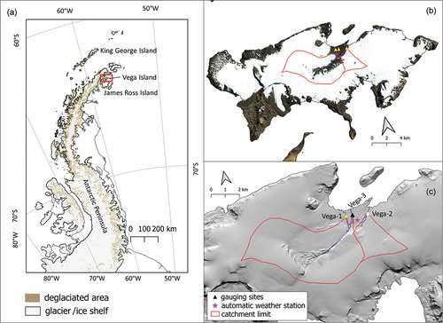
Vega-1 and Vega-3 drain the same glacier (Devil’s Bay glacier), with adjacent parts of the dome glacier. Therefore, distinguishing between the two catchments is difficult, and this is further complicated by the morphology of the till plain at the front of the glacier snout. The two streams are positioned next to each other; Vega-3 drains the eastern part of the glacier, whereas the Vega-1 stream originates from a throughflow in the glacier frontal moraine. The Vega-1 catchment reaches an altitude of 600 m a.s.l. on top of the dome glacier, whereas Vega-3 is mainly situated in the deglaciated volcanic mesa area, reaching an altitude of approximately 350 m a.s.l. in its glaciated parts. Moreover, the two streams flow through a large braidplain that, during the study period, was overlain by a snowpack, where signs of possible bifurcation were found at the end of the study. In this context, the two streams can be considered part of one common catchment (Fig. 1).

The Vega-2 stream is distinct from the other two glacial streams and is fed by a sub-glacial network of channels from beneath the dome glacier (approximately 420 m a.s.l.) along its western margin. We have delimited ts catchment based on the surface topography of the glacier, which does not necessarily correspond to the actual catchment area taking into account the sub-glacial topography. It is, therefore, essential to take this catchment area with some caution; and the true extent of the catchment may be significantly different.

2 Material and methods

The study was carried out during the austral summer of 2013; the measurement equipment was installed and used between 17 January and 21 February 2013. All the reported times are in UTC.

2.1 Discharge time series

We chose three gauging sites to measure discharge and hydrostatic pressure in the streams. We primarily considered the stability of the cross-profile when choosing these sites, to ensure there was as little turbulence in the water as possible. At each site, we installed a Heron DipperLog automatic pressure sensor (accuracy of ± 0.05%), which measured hydrostatic pressure at 15-minute intervals. Using these pressure data, we were able to calculate the water level at each site by adjusting the measurements for atmospheric pressure, which was measured at a nearby air pressure gauge. We then converted these water levels into river discharge using rating curves.

To produce the rating curves, we measured discharge manually at each site using an ADCP FlowTracker handheld device (ISY Sontek). We performed six manual discharge measurements at the Vega-1 gauging site, nine at the Vega-2 gauging site, and six at the Vega-3 gauging site. The rating curve correlation coefficients were 0.98 for Vega-1, 0.99 for Vega-2 and 0.92 for Vega-3 (Fig. 2). All the rating curve fittings are statistically significant (p < .001). The measured discharge covered 81% of the whole range of calculated discharges (13–94%) in Vega-1, 90% (5–95%) in the case of Vega-2 and 85% (6–91%) for Vega-3. The uncertainty calculations followed the International Organization for Standardization (ISO) 748 method (ISO 2003) for manual discharge measurements and the ISO 25377 procedure (ISO 2007) for rating curve relative uncertainty. The overall calculated discharge time series uncertainty (including manual discharge measurement and rating curve calculation) is 11.6% for Vega-1, 13.1% for Vega-2 and 14.8% for Vega-3. These reported uncertainties are later applied also for the uncertainty range of the glacier ablation calculations (see the section “Glacier ablation”).

Figure 2. Rating curve used for calibration of the discharge time series plotted with its uncertainty range: (a) Vega-1; (b) Vega-2; (c) Vega-3.

The catchment boundaries were delimited using the Reference Elevation Model of Antarctica (REMA) Digital Elevation Model (DEM) 2 m resolution strips (Howat et al. 2019). The catchments for Vega-1 and Vega-3 were difficult to distinguish as these two streams were draining the same glacier within unconstrained channels along the glacier till plain. Additionally, the river network was covered with a semi-permanent snowpack for most of the field campaign with possible bifurcation observed between the two river channels. Therefore, the overall statistics related to these catchments were unreliable and, instead, we produced an ensemble of discharge data from the two streams that encompasses all streams flowing from the glacier.

2.2 Atmospheric variables

Air temperature and air pressure were measured at 15-minute intervals using a MiniLog Temp (accuracy ± 0.15°C, EMS Brno, CZ) and a TMAG 518 N4H barometer (accuracy ± 0.5 hPa; CRESSTO, CZ) respectively. The automatic weather station was in the deglaciated part of the study area near the three gauging sites (63.824231°S, 57.322578°W) (Fig. 1).

2.3 Glacier ablation

Discharge measured at the Vega-1 gauging site represents the runoff from the catchment of the GBD glacier (see Fig. 1). It was thus possible to recalculate the measured discharge to obtain daily surface ablation time series in terms of melted water equivalent (mm w.e.). The total volume of runoff during the study period divided by the glacier surface area (12.9 km² as reported by Marinsek and Ermolin (2015)) provides the total runoff depth (mm) in the study period. The same recalculation is often used in water balance studies and modelling applications (e.g. Gallo 2007, Gyasi-Agyei 2019, Reynolds et al. 2020). The uncertainty in the ablation calculation comes from the uncertainty in the discharge time series, which was calculated as 11.6% for Vega-1.

3 Results

The mean air temperature during the study period was 0.9°C and the daily mean ranged from 8.5°C to −7.0°C. The maximum air temperature reached 13.3°C on 20 January, and it exceeded 10°C on another eight days during the study period. At the same time, the minimum daily temperature dropped below 0°C on 28 of the 36 days, with a minimum of −8.2°C on 19 February. The mean daily amplitude of the temperatures was 7.6°C with a maximum daily amplitude of 14.9°C (25 January) and a minimum daily amplitude of 1.4°C (15 February).

The discharge time series cover more than one month during the peak of the 2013 summer (Fig. 3). All three of the streams studied exhibited a similar temporal pattern of discharge despite their differences in catchment topography. All of the streams were influenced by high glacier coverage, demonstrated by high discharge variability and a strong diurnal regime because of variations in air temperature.

Figure 3. Discharge time series for all the three streams studied over the period 17 January–21 February 2013.

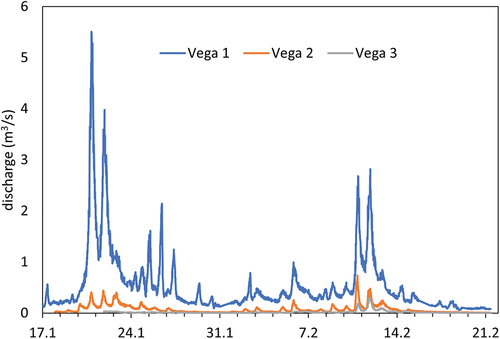
The mean discharge during the whole measurement period was 0.523 m³s⁻¹ for Vega-1, 0.076 m³s⁻¹ for Vega-2, and 0.020 m³s⁻¹ for Vega-3. The highest manually recorded discharge was 1.499 m³s⁻¹ at 3.00 pm on 21 January 2013 on the Vega-1 stream. This was also the day with the second highest calculated discharge, with its peak (3.977 m³s⁻¹) at 9:22 pm. The highest calculated discharge occurred the preceding day (20 January 2013 at 8.52 pm) with the maximum reaching up to 5.510 m³s⁻¹. The peak discharge was likely caused by the melting of snow that fell during a massive snowstorm in the preceding days. The Vega-2 stream experienced a similar discharge pattern, although the maximum discharge of 0.737 m³s⁻¹ was recorded on 10 February 2013 at 8.52 pm. The maximum discharge on the Vega-3 stream was also recorded during the second seasonal maximum in February. The maximum discharge of 0.302 m³s⁻¹ was recorded on 11 February 2013, at 9.37 pm. All the studied streams experienced their minimum discharge at the end of the study period after the sudden drop in air temperatures and a persistent cold span with below-zero temperatures for several consecutive days. The discharge in Vega-3 was very low, at only 0.002 m³s⁻¹; similarly, Vega-2 had a discharge of only 0.010 m³s⁻¹. In contrast, Vega-1 had a relatively high discharge of 0.050 m³s⁻¹, probably because it continued to be fed by extensive sub-glacial drainage.

The water temperature in all three streams (Fig. 4) was relatively stable and usually fluctuated around 1–2°C with an important decrease at the end of the study period. The lowest mean water temperature (0.79°C) was recorded in the Vega-1 stream, whereas the highest mean water temperature was recorded in Vega-3 stream (2.0°C); Vega-2 mean water temperature was 0.9°C. The lowest water temperature recorded in Vega-1 is likely to be affected by the highest discharge of the stream and the short river channel between the outlet of the glacier and the gauging site. In contrast, the water temperature of Vega-3 was influenced by its long river channel and the high proportion of deglaciated area in its catchment. The meltwater from the volcanic mesa and adjacent slopes had sufficient time to warm up before reaching the measurement site.

Figure 4. Discharge, water temperature and air temperature for (a) Vega-1, (b) Vega-2 and (c) Vega-3 over the study period: 17 January–21 February 2013.

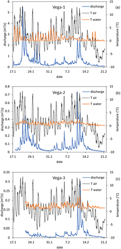
Two periods of high discharge recorded in Vega-1 and Vega-2 coincided with elevated air temperatures around 20 January and 10 February 2013. The first high discharge period occurred before the start of the measurement on Vega-3, therefore only the second high discharge period is recorded here. The maximum water temperature was recorded in Vega-3 (6.0°C) on 11 February at 5.52 pm; the maximum water temperature in Vega-1 was reached on 17 January at 5.07 pm (5.81°C). The highest water temperature in Vega-2 was recorded on 10 February at 4.37 pm (2.69°C). The water temperature is strongly correlated with air temperature and follows a diurnal cycle. However, the highest recorded water temperature did not always coincide with the period of highest discharge or highest air temperature. A possible mechanism for this is that the relatively high specific heat capacity of water means water is slow to respond to small changes in air temperature. This is especially apparent in Vega-1 where the days with peak discharge had only low maximum water temperatures. When a large increase in air temperature was observed (e.g. on 31 January, Fig. 4(a)) an increase in water temperature was also seen. The low mean water temperature and low variability of Vega-2 might be explained by its short river channel and direct outflow of cold meltwater from the sub-glacial hydrological network. This did not allow the water to be heated significantly and resulted in the lowest maximum water temperature when compared to the other two streams (Fig. 4(b)). The low variability in water temperature in the case of Vega-3, despite its low discharge, is likely a result of the sensor being in a relatively deep pool of water (to ensure robust water level measurements could be taken). This resulted in a low fluctuation of the water temperature, usually between 1.5 and 3.5°C, with only two exceptions, on 10 and 11 February, where the temperature exceeded 5°C (Fig. 4(c)).

3.1 The effect of air temperature on water discharge and water temperature

3.1.1 Diurnal regime

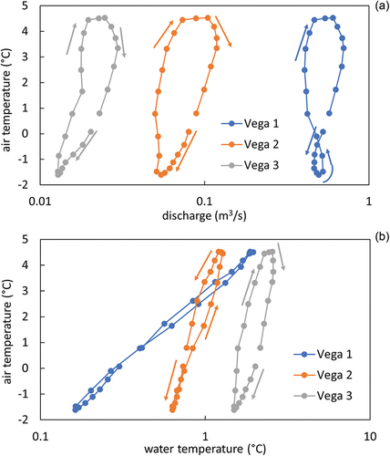
The discharge and water temperature appear to follow a hysteresis loop when plotted against air temperature. This relationship is particularly clear for discharge (Fig. 5(a)), where only minor deviations in the shape of the curve can be observed, most notably in the data from Vega-1. The loops are more deformed in the case of water temperature (Fig. 5(b)), but a well-developed loop can be observed for Vega-3, with a clockwise direction. This implies that there is a delayed reaction of water temperature to changes in air temperature (Fig. 5(b)).

Figure 5. Hysteresis loop of discharge/air temperature and water temperature/air temperature based on mean hourly data from the whole study period.

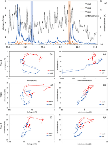
Two days with very different air temperatures were chosen to demonstrate the impact of atmospheric forcings on discharge and water temperature. The first, 26 January, represents a cold day with an average temperature of 0°C (with a minimum of −6.9°C and maximum of 7.0°C), whereas 10 February represents a warm day with an average air temperature of 7.3°C (with a minimum of 2.8°C and a maximum of 12.6°C) (Fig. 6(a)). A well-developed clockwise hysteresis loop is clearly visible on the warm day, for both discharge and water temperature. This pattern is, however, not observed on the cold day, where a clear clockwise hysteresis is recorded only for Vega-2 discharge and Vega-3 water temperature. Vega-1 and Vega-3 discharge shows a transition mode of hysteresis. Vega-1 starts as an anti-clockwise loop, but it turns clockwise at the end of the day. In contrast, Vega-3 starts as a clockwise loop but quickly transforms into an anti-clockwise loop. Vega-2 water temperature hysteresis has a deformed anti-clockwise direction whereas the Vega-1 water temperature loop is deformed by the 0°C values for a large part of the day.

Figure 6. Hysteresis loop of discharge/air temperature and water temperature/air temperature during cold and warm days (26 January and 10 February, respectively).

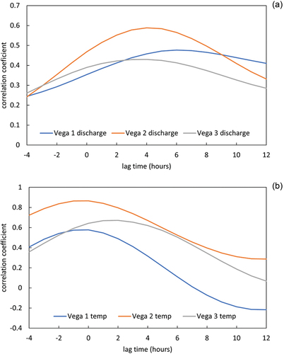
The timing of the discharge and water temperature within the diurnal regime is illustrated in Fig. 7. The lag time of discharge differs between Vega-1 (six hours) and the other two streams (four hours). This might explain the deformed shape of the hysteresis loop of Vega-1 in Fig. 7(a). In contrast, there is no lag time when analysing water and air temperature (Vega-1 and Vega-2) and only two hours’ lag time in the case of Vega-3. This lag time could be explained by the longer flowpath of the meltwater reaching the gauging profile from the deglaciated volcanic mesa and adjacent slopes. The flowpath of meltwater reaching the Vega-1 and Vega-2 profiles is extremely short and avoids the warm-up effect during the flow. The two streams are fed almost directly from the glacier; therefore, we observed no effect on the lag time of water temperature. In contrast, the flowpath including the supraglacial and sub-glacial drainage network is long enough to produce the four- to six-hour lag time of discharge. The peak discharge follows up to six hours after the air temperature maximum.

Figure 7. Lag time of (a) discharge/air temperature and (b) water temperature/air temperature for the whole study period: 17 January – 21 February 2013.

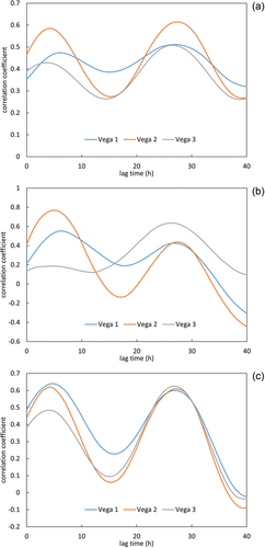
The cross-correlation analysis (Fig. 8) of the detailed 15-minute measurements over the study period showed the highest coefficients with lags between 26.5 hours (Vega-1) and 27.5 hours (Vega-2). Furthermore, we selected two 7-days case study periods. Period 1, between 1 and 7 February, had relatively low mean discharges ranging from 0.01 m³s⁻¹ (Vega-3) to 0.35 m³s⁻¹ (Vega-1). Discharges during Period 2 (8 and 14 February) were almost double this, falling between 0.04 m³s⁻¹ (Vega-3) and 0.67 m³s⁻¹ (Vega-1). The response of discharges to air temperature variability in Period 1 was relatively fast in Vega-1 and Vega-2 where the maximum correlations were detected with a lag of 5 to 6 hours whereas the maximum correlation of 27 hours was observed on Vega-3 (Fig. 8(b)). The situation from Period 2 similarly showed the maximum correlations with a five- to six-hour lag (Vega-1 and Vega-2); however, the correlations with 25 to 27 hours’ delay reached almost the same values (Fig. 8(c)).

Figure 8. Cross-correlation coefficients between air temperature and water discharges on streams Vega-1–3 in the periods of (a) 17 January to 21 February 2013, (b) 1 to 7 February 2013 and (c) 8 to 14 February 2013.

3.1.2 Seasonal effect of air temperature

The mean daily discharges of the studied streams responded with a one-day time lag to air temperature variability. The strongest relationship, expressed by a non-linear exponential function, was observed for Vega-1 (R² = 0.68) while the lowest was observed for Vega-3 (R² = 0.54) (Fig. 9). The regression for cases without a one-day time lag was notably lower, between R² = 0.49 (Vega-1) and R² 0.31 (Vega-3).

Figure 9. The effect of air temperature on discharges in Vega-1–3 streams. The discharges are 1-day delayed.

We observed a weak to moderate relationship expressed by a non-linear function between air temperature and water temperature (R² = 0.12 to 0.70). The warmest days (> 6°C) were typically associated with rather low water temperatures of between 0.5 and 1.0°C. The highest water temperatures (around 2.0°C in the case of Vega-1) were observed only on the days with slightly above-average air temperature (2 to 4°C) and discharges (Fig. 10(a)). In such conditions, the streams with lower water levels were heated by the atmosphere much more effectively. This is especially the case for Vega-1, where the correlation coefficient was the weakest. Vega-3, however, showed a more consistent trend with the highest water temperatures recorded. Vega-2 experienced the lowest water temperatures and the closest fit with air temperature. This is likely due to its short water course out of the glacier system. Importantly, positive water temperatures (indicating the flow of liquid water) were observed down to very low air temperatures of −7°C.

Figure 10. The relationship between air temperature and water temperature for (a) Vega-1, (b) Vega-2 and (c) Vega-3.

3.2 Calculated ablation of the GBD

The ablation of the GBD glacier based on the recalculation of the discharge time series of the Vega-1 stream shows a total ablation rate of 124.5 ± 14.4 mm w.e. during the study period. The variability of the daily ablation rate corresponded with the variability of runoff and varied from 0.5 to 14.7 mm w.e.day⁻¹.

4 Discussion

4.1 Runoff dynamics

The average discharge recorded at the Vega-1 gauging site (0.523 m³s⁻¹) is one of the highest recorded discharges in Antarctica. Kavan et al. (2017) reported the average discharge for Bohemian Stream (on neighbouring James Ross Island) as 0.19 m³s⁻¹ during the 2015 austral summer, and Kavan (2022) reported it as only 0.14 m³s⁻¹ during the 2018 austral summer. Stott and Convey (2021) calculated the average discharge of the Orwell Glacier meltwater stream on Signy Island as only 0.048 m³s⁻¹. Szilo and Bialik (2017) studied bedload transport and discharge on the outlet of the Baranowski Glacier (King George Island) and found the maximum discharge to be only 0.719 m³s⁻¹, with average discharge likely to have been less than 0.2 m³s⁻¹. Falk et al. (2018) used a modelling approach to estimate mean discharge in two small creeks in Potter Cove (King George Island) and found it to be 0.44 m³s⁻¹ and 0.55 m³s⁻¹ respectively. Inbar (1995) found an average discharge of 0.02 m³s⁻¹ at a gauging site on Deception Island.

Apart from the Antarctic Peninsula and Maritime Antarctica, fluvial dynamics have largely been previously studied in the McMurdo Dry Valleys region. Hawke and McConchie (2001) documented the average discharge as below 0.2 m³s⁻¹ in Miers Valley. The average recorded discharge on Onyx River (the largest in the McMurdo Dry Valleys region) in the early 1970s was around 0.5 m³s⁻¹, with the maximum discharge reaching up to 4 m³s⁻¹ (Shaw and Healy 1980). Chinn and Mason (2016) reported the mean discharge during the flow days between 1972 and 1991 to approximately 0.64 m³s⁻¹. Such characteristics are very similar to those reported from Vega-1, with the maximum discharge reaching up to 5.510 m³s⁻¹.

The Onyx River is often considered to be the largest in Antarctica, which is certainly true considering its total catchment area. However, the discharge of the Onyx is rather low, making it more comparable to streams in smaller deglaciated areas of Antarctica, where warmer temperatures lead to more intensive snow/glacier melt. To compare the Antarctic catchments and their runoff production it is necessary to keep in mind that not only the catchment area but also the duration of the flow season is different and may vary considerably. There may be only a few weeks of runoff in McMurdo Dry Valleys, but it may last up to a few months in the case of Maritime Antarctica. For that reason, we also include a comparison of the aforementioned catchments in terms of their area, typical flow season length and basic runoff characteristics (Table 1). Using the flow depth parameter (mm day⁻¹) can help us to compare the runoff production in different catchments; however, this is strongly affected by the reliability of catchment area delimitation. This is sometimes rather difficult due to complex and usually unknown sub-glacial topography. This might be the case for the Vega-2 stream (where the actual catchment area is probably smaller) and certainly for the Orwell Glacier stream (Stott and Convey 2021), where the actual catchment area is probably much larger.

Table 1. Comparison of available discharge measurements in Antarctica. Catchment areas marked with (*) were not provided in the original reference; the estimate was thus made based on the available Reference Elevation Model of Antarctica Digital Elevation Models; ^A the study period was not precisely stated; ^B there were multiple study seasons between 1972 and 1991.

Stream	Catchment area (km^2)	Flow season length (months)	Study period	Observation length (days)	Mean discharge (m^3s^−1)	Flow depth (mm day^−1)	Annual runoff volume (million m^3)	Reference
Vega-1	12.9	3–4	17 January–21 February 2013	36	0.523	3.50	4.74	This study
Vega-2	6	3–4	17 January–21 February 2013	36	0.076	1.09	0.69	This study
Algal Stream	2.82	4	8 January–18 February 2015	42	0.06	1.84	0.62	Kavan et al. (2017)
Bohemian Stream	6.47	4	8 January–18 February 2015	42	0.19	2.54	1.97	Kavan et al. (2017)
Bohemian Stream	6.47	4	17 January–28 February 2018	43	0.14	1.87	1.45	Kavan (2022)
Orwell Glacier	0.32	6	5 December 2019–21 February 2020	79	0.048	12.96	0.75	Stott and Convey (2021)
Fosa Stream	10*	5–6	8 January–11 February 2016	35	0.2	1.73	2.85	Szilo and Bialik (2017)
Potter Stream	8.42	5–6	25 January–18 March 2011	53	0.44–0.55	4.51–5.64	6.27–7.84	Falk et al. (2018)
Deception Island	0.65	3	23 January–8 March 1991	45	0.02	2.66	0.16	Inbar (1995)
Miers Stream	12*	2–3	end November–mid February^A	90	0.1	0.72	0.65	Hawke and McConchie (2001)
Onyx River	550*	2	mid December–mid February^B	65	0.64	0.10	3.32	Chinn and Mason (2016)

The two other gauging sites (Vega-2 and Vega-3) show considerably lower discharge, although Vega-2 is draining part of the adjacent ice cap. The lower discharge could be explained by the fact that most of the meltwater originated in the sub-glacial environment, which may drain a smaller area than delimited by the surface drainage area.

River discharge shows a good correlation with air temperature when a one-day lag is accounted for. A possible mechanism for this time lag is that the sub-glacial network is composed of a complex series of cavities and channels, so it may take some time for surface melt to percolate through the ice and into the basal river channels (Flowers 2015). Preferential flow through cavities (slow) or channels (fast) may also vary during the ablation season, causing a highly variable runoff response (Nanni et al. 2020). Therefore, we can observe the difference in the hydrological dynamics between a glacier-sourced river system (this study) and a permafrost/snowfield-fed water system on James Ross Island. In a catchment with less glacier cover, the lag time between air temperature and discharge is shorter (Kavan et al. 2017). A similar correlation between discharge and atmospheric parameters with a time lag of 0–3 days was reported from a glacierized basin in the Himalayas (Singh et al. 2000). Yang and Peterson (2017) found a large variety of water temperature regimes in Mackenzie and Yukon basins, where the time lag ranged from 1 to 40 days depending on the areal extent of the basin and presence of large lakes on the water stream. In contrast, Falk et al. (2018) observed a strong correlation between discharge with surface air temperature on King George Island, indicating a short lag time. The clear hysteresis pattern of discharge and air temperature confirms the relatively long time lag. This relationship may be deformed during cold days with negative air temperatures when the delayed reaction is likely caused by the sub-glacial hydrological system with large inertia. On these days, sub-glacial runoff production is probably the primary source of meltwater runoff in front of the glacier, as is the case for Vega-1 (Fig. 5(b)).

4.2 Water temperature

The meltwater draining the glacier is just above 0°C in temperature. Most of the heat energy within the glacier system (no matter whether it is in the supraglacial or sub-glacial environment) is used during melting, which is an endothermic process, rather than raising the temperature of the water (Constantz 1998). The energy was only transferred from the atmosphere to the water in a small portion of the river downstream of the glacier outlet. Cadbury et al. (2008) reported a water temperature rise of 0.6°C km⁻¹ along the length of a stream in a glacierized basin in New Zealand. Similarly, Gao et al. (2017) reported a water temperature rise from the glacier margin of 0.13–0.28°C km⁻¹ for several catchments in the Tibetan Plateau. This also shows the impact of different catchment properties such as bedrock and soil properties, or catchment gradient. The enhanced glacier melt during warm days usually results in lower water temperatures (e.g. van Vliet et al. 2013, Du et al. 2022) as the larger volume of meltwater also has a higher thermal capacity (Milner et al. 2017). Higher water temperatures were, therefore, observed during days with low meltwater production and low discharge, which enabled a more effective heat transfer in the low volume of water in the stream (Collins 2009). A similar cooling effect was even seen during warm days with high incoming shortwave radiation in some glacierized Alpine catchments (Williamson et al. 2019). However, Williamson et al. (2019) reported that the water temperature was also controlled by the stream surface area. The hysteresis loops presented in Fig. 5 illustrate well the conditions of each catchment. The clockwise hysteresis in Vega-3 reflects the cooling effect of glacial meltwater (Fellman et al. 2014). There is no apparent hysteresis pattern in the case of Vega-1. This is probably caused by massive sub-glacial meltwater production, which is not directly and immediately affected by fluctuations in air temperature. A clear hysteresis pattern is visible during warm days (Fig. 5(c)). In contrast, hysteresis is non-existent during cold days, when meltwater draining the sub-glacial network exits the glacier at 0°C and is not warmed considerably before reaching the gauging site. Surprisingly, Vega-2 shows a counter-clockwise hysteresis, which is at odds with the extremely high glacier coverage of the catchment. This could be explained by the extremely low water temperature (usually below 1°C), long lag time, and rather complex sub-glacial meltwater transport resulting in the water temperature being less sensitive to changes in air temperature.

Despite the short watercourse of the streams studied on Vega Island, they were usually inhabited by several microorganisms (e.g. Bulínová et al. 2020)T. Notably, the data of discharges and water temperature show that streams remain active even in cold conditions with air temperatures around −7 to −8°C. This threshold temperature is about 2–4°C lower than was observed on James Ross Island (Kavan et al. 2017).

4.3 Ablation of GBD

The calculated ablation rate of 124.5 ± 13.7 mm w.e. for the GBD glacier during the study period (17 January–21 February) covered only part of the ablation season but in the overall view corresponded well to the long-term net mass balance (approximately −20 cm/year) reported by Marinsek and Ermolin (2015). The study period did not cover the whole ablation period, which may extend up to 8–10 weeks, therefore the summer ablation calculated from the whole runoff/ablation period would have been higher. The reason for the relatively low ablation rate could also be that the 2013 austral summer was one of the coldest in recent decades (Oliva et al. 2017), which was also reflected in the most positive mass balance observed on Whisky Glacier and Davies Dome on the nearby James Ross Island in the period 2009–2015 (Engel et al. 2019). Therefore, we argue that runoff from the glacierized catchment measured directly by standard hydrological methods may serve as a useful proxy for the estimation of the overall ablation rate of the glacier.

The proposed method of calculating the ablation rate based on runoff can be successfully used in regions where sublimation accounts only for a minor part of the total glacier mass loss. Some of the glaciers located in a dry continental climate with very low air temperatures are losing most of their mass by sublimation (e.g. McMurdo Dry Valleys in Bliss et al. 2011; Andes in MacDonell et al. 2013, Ayala et al. 2017). However, these examples account for glaciers in regions where the air temperature rarely exceeds 0°C, which is not the case for the GBD. The approach may be useful for different land-terminating glaciers in the Antarctic Peninsula region, where ablation is the principal cause of glacier mass loss and where the outflow of the glaciers is well defined. van Lipzig et al. (2004) estimated the sublimation in the Antarctic Peninsula region to be 9%. This sublimation rate also includes large areas of high-elevated ice caps; therefore, the sublimation in low-lying glaciers is likely to be significantly lower. This might be the case with the neighbouring James Ross Island, where routine glaciological observations are carried out using classic techniques (e.g. Engel et al. 2018, 2022).

The overall glacier mass balance is the result of the difference in accumulation and ablation (Benn and Evans 2010). The estimation of the ablation rate based on runoff measurement together with direct glaciological measurements of mass balance can therefore serve as a basis for the completion of the mass balance equation, where the accumulation rate is unknown. The accumulation rate is often difficult to measure as it is spatially highly variable, both in relatively small glaciers (McGrath et al. 2018) and in the case of the whole ice sheets (Dattler et al. 2019). Large differences in snow accumulation were also observed among individual glaciers on the neighbouring James Ross Island, where the snow accumulation rate is driven by the prevailing wind direction and local topography (Kavan et al. 2020b). Large-scale patterns of precipitation exhibit high spatial and temporal variability in the whole of Antarctica (compare e.g. Robinson et al. 2018, Medley and Thomas 2019, Vignon et al. 2021). As a result, reliable precipitation estimates are relatively scarce, and such estimates are subject to large uncertainties arising from point observations (Tang et al. 2018) or low spatial resolution of remote sensing data (Souverijns et al. 2018). The James Ross Archipelago, for example, has a large range of estimated precipitation: between 300 and 700 mm w.e.year⁻¹ (e.g. van Lipzig et al. 2004, van Wessem et al. 2016, Palerme et al. 2017). Therefore, we see great potential in combining total mass balance (glaciological measurements) with ablation rate (runoff measurement) to estimate the accumulation rate over the glacier surface. Moreover, such measurements would avoid the uncertainty arising from a single-point measurement while integrating the spatial variability of accumulated precipitation.

5 Conclusions

Overall, this study highlights the importance of runoff observations from the Antarctic region, where such studies are scarce. Data from three streams on Vega Island revealed high variability in flow dynamics. The recorded discharge was among the highest documented in Antarctic streams, in terms of both the maximum discharge (5.510 m³s⁻¹) and the mean long-term discharge (0.523 m³s⁻¹). We identify air temperature as the key control on both discharge and water temperature. The discharge persisted for several days even when the air temperature dropped to −7°C, suggesting the large momentum of the glacier system and the large contribution of the sub-glacial hydrological environment to the overall runoff. Furthermore, the runoff measured on the outflow of the glacier allowed us to calculate the glacier ablation rate. Compared to long-term glaciological observations, we show that this method is a reliable way to estimate ablation rate. We propose that a suitable way to calculate the mass balance of a remote glacier in the field would be to use a combination of direct glaciological measurement for mass balance, with ablation rate estimates based on runoff measurement, to calculate the accumulation rate. We argue that such an approach may overcome the methodological limitations of using single-point measurements, taking into account the whole glacier surface as a “measurement site.” This could help to avoid spatial and temporal variability of precipitation and provide us with reliable estimates of accumulation, i.e. precipitation.

Acknowledgements

Special thanks are given to the staff of J. G. Mendel Station for the field assistance, as well as to Marcos A. E. Chaparro and all field members of the Picto project.

Disclosure statement

No potential conflict of interest was reported by the authors.

Additional information

Funding

This work was supported by the Czech Science Foundation [project no. GA20-20240S]; the Ministry of Education, Youth and Sports of the Czech Republic [project no. LM2015078]; the Instituto Antárctico Argentino (logistical and financial support for the field campaign); the PICTO project [2010-0096]; and the SVELTA project [UMO-2020/37/K/ST10/02852]. CDS was in receipt of a PhD studentship from the Leeds-York-Hull Natural Environment Research Council (NERC) Doctoral Training Partnership (DTP) Panorama [under grant no. NE/S007458/1].

References

- Ayala, A., et al., 2017. Melt and surface sublimation across a glacier in a dry environment: distributed energy-balance modelling of Juncal Norte Glacier, Chile. Journal of Glaciology, 63, 803–822. doi:10.1017/jog.2017.46.
- Benn, D. and Evans, D.J.A., 2010. Glaciers and glaciation. 2nd ed. Routledge, 816.
- Bergstrom, A., et al., 2021. Long-term shifts in feedbacks among glacier surface change, melt generation and runoff, McMurdo Dry Valleys, Antarctica. Hydrological Processes, 35, e14292. doi:10.1002/hyp.14292.
- Björck, S., et al., 1996. Late Holocene palaeoclimatic records from lake sediments on James Ross Island, Antarctica. Palaeogeography, Palaeoclimatology, Palaeoecology, 121, 195–220. doi:10.1016/0031-0182(95)00086-0.
- Bliss, A., Cuffey, K., and Kavanaugh, J., 2011. Sublimation and surface energy budget of Taylor Glacier, Antarctica. Journal of Glaciology, 57, 684–696. doi:10.3189/002214311797409767
- Brown, L.E., Hannah, D.M., and Milner, A.M., 2005. Spatial and temporal water column and streambed temperature dynamics within an alpine catchment: implications for benthic communities. Hydrological Processes, 19 (8), 1–20. doi:10.1002/hyp.5590.
- Bulínová, M., et al., 2020. Comparison of diatom paleo-assemblages with adjacent limno-terrestrial communities on Vega Island, Antarctic Peninsula. Water, 12, 1340. doi:10.3390/w12051340.
- Cadbury, S.L., et al., 2008. Stream temperature dynamics within a New Zealand glacierized river basin. River Research and Applications, 24 (1), 68–89. doi:10.1002/rra.1048.
- Čejka, T., et al., 2020. Timing of the neoglacial onset on the North-Eastern Antarctic Peninsula based on lacustrine archive from Lake Anónima, Vega Island. Global and Planetary Change, 184, 103050. doi:10.1016/j.gloplacha.2019.103050.
- Chaparro, M.A.E., et al., 2017. Sedimentary analysis and magnetic properties of Lake Anónima, Vega Island. Antarctic Science, 29, 429–444. doi:10.1017/S0954102017000116.
- Chinn, T. and Mason, P., 2016. The first 25 years of the hydrology of the Onyx River, Wright Valley, Dry Valleys, Antarctica. Polar Record, 52, 16–65. doi:10.1017/S0032247415000212
- Chu, V.W., 2014. Greenland ice sheet hydrology: a review. Progress in Physical Geography, 38, 19–54. doi:10.1177/0309133313507075
- Collins, D.N., 2009. Seasonal variations of water temperature and discharge in rivers draining ice-free and partially-glacierised Alpine basins. 17th International Northern Research Basins Symposium, Iqaluit-Pangnirtung-Kuujjuaq, Canada, 67–74.
- Constantz, J., 1998. Interaction between stream temperature, streamflow, and groundwater exchanges in alpine streams. Water Resources Research, 34, 1609–1615. doi:10.1029/98WR00998
- Daigle, A., Jeong, D.I., and Lapointe, M.F., 2015. Climate change and resilience of tributary thermal refugia for salmonids in eastern Canadian rivers. Hydrological Sciences Journal, 60, 1044–1063. doi:10.1080/02626667.2014.898121
- Dattler, M.E., Lenaerts, J.T.M., and Medley, B., 2019. Significant spatial variability in radar-derived west Antarctic accumulation linked to surface winds and topography. Geophysical Research Letters, 46, 13126–13134. doi:10.1029/2019GL085363
- Docherty, C.L., et al., 2019. Arctic river temperature dynamics in a changing climate. River Research and Applications, 35, 1212–1227. doi:10.1002/rra.3537.
- Du, X., Silwal, G., and Faramarzi, M., 2022. Investigating the impacts of glacier melt on stream temperature in a cold-region watershed: coupling a glacier melt model with a hydrological model. Journal of Hydrology, 605, 127303. doi:10.1016/j.jhydrol.2021.127303
- Engel, Z., et al., 2018. Surface mass balance of small glaciers on James Ross Island, north-eastern Antarctic Peninsula, during 2009–2015. Journal of Glaciology, 64, 349–361. doi:10.1017/jog.2018.17.
- Engel, Z., et al., 2019. Surface mass balance of Davies Dome and Whisky Glacier on James Ross Island, north-eastern Antarctic Peninsula, based on different volume-mass conversion approaches. Czech Polar Reports, 9, 1–12. doi:10.5817/CPR2019-1-1.
- Engel, Z., et al., 2022. Persistent mass loss of Triangular Glacier, James Ross Island, north-east Antarctic Peninsula. Journal of Glaciology, 69, 27–39. doi:10.1017/jog.2022.42.
- Falk, U., Silva-Busso, A., and Pölcher, P., 2018. A simplified method to estimate the run-off in Periglacial Creeks: a case study of King George Islands, Antarctic Peninsula. Philosophical Transactions of the Royal Society A, 376, 20170166. doi:10.1098/rsta.2017.0166
- Fellman, J.B., et al., 2014. Stream temperature response to variable glacier coverage in coastal watersheds of Southeast Alaska. Hydrological Processes, 28, 2062–2073. doi:10.1002/hyp.9742.
- Flowers, G.E., 2015. Modelling water flow under glaciers and ice sheets. Proceedings of the Royal Society A: Mathematical, Physical and Engineering Sciences, 471, 20140907. doi:10.1098/rspa.2014.0907
- Foreman, C.M., Wolf, C.F., and Priscu, J.C., 2004. Impact of episodic warming events on the physical, chemical and biological relationships of lakes in the McMurdo Dry Valleys, Antarctica. Aquatic Geochemistry, 10, 239–268. doi:10.1007/s10498-004-2261-3
- Fountain, A., et al., 2004. Evolution of cryoconite holes and their contribution to meltwater runoff from glaciers in the McMurdo Dry Valleys, Antarctica. Journal of Glaciology, 50, 35–45. doi:10.3189/172756504781830312.
- Gallo, E.L., 2007. Land cover controls on summer discharge and runoff solution chemistry of semi-arid urban catchments. Journal of Hydrology, 485, 37–53. doi:10.1016/.jhydrol.2012.11.054
- Gao, T., et al., 2017. Stream temperature dynamics in Nam Co basin, southern Tibetan Plateau. Journal of Mountain Science, 14 (1), 2458–2470. doi:10.1007/s11629-016-4234-6.
- García-Rodríguez, F. et al., 2021. Centennial glacier retreat increases sedimentation and eutrophication in Subantarctic periglacial lakes: A study case of Lake Uruguay. The Science of the Total Environment, 754, 142066. doi:10.1016/j.scitotenv.2020.142066.
- Gerrish, L., 2020. High resolution vector polygon seamask for areas south of 60S (7.3) [Data set]. UK Polar Data Centre, Natural Environment Research Council, UK Research & Innovation. doi:10.5285/0640f7af-516e-4cf3-9e09-8a6cd9f4b150.
- Gonzales, S. and Fortuny, D., 2018. How robust are the temperature trends on the Antarctic Peninsula? Antarctic Science, 30 (5), 322–328. doi:10.1017/S0954102018000251.
- Gyasi-Agyei, Y., 2019. Propagation of uncertainties in interpolated rainfields to runoff errors. Hydrological Sciences Journal, 64, 587–606. doi:10.1080/02626667.2019.1593989
- Harmon, R.S., et al., 2021. Geochemistry of contrasting stream types, Taylor Valley, Antarctica. GSA Bulletin, 133, 425–448. doi:10.1130/B35479.1.
- Hawke, R.M. and McConchie, J.A., 2001. Bedload transport in a meltwater stream, Miers Valley, Antarctica: controls and prediction. Journal of Hydrology (New Zealand), 40 (1), 1–18.
- Hodson, A., et al., 2017. Climatically sensitive transfer of iron to maritime Antarctic ecosystems by surface runoff. Nature Communications, 8, 14499. doi:10.1038/ncomms14499.
- Howat, I.M., et al., 2019. The reference elevation model of Antarctica. The Cryosphere, 13, 665–674. doi:10.5194/tc-13-665-2019.
- Hrbáček, F., et al., 2017. Active layer monitoring at CALM-S site near J.G.Mendel Station, James Ross Island, eastern Antarctic Peninsula. Science of the Total Environment, 601–602, 987–997. doi:10.1016/j.scitotenv.2017.05.266.
- Hugonnet, R., et al., 2021. Accelerated global glacier mass loss in the early 21st century. Nature, 592, 726–731. doi:10.1038/s41586-021-03436-z.
- Huss, M. and Hock, R., 2018. Global-scale hydrological response to future glacier mass loss. Nature Climate Change, 8, 135–140. doi:10.1038/s41558-017-0049-x
- Inbar, J., 1995. Fluvial morphology and streamflow on Deception Island, Antarctica. Geografiska Annaler. Series A, Physical Geography, 77, 221–230. doi:10.2307/521331
- ISO, 2003. ISO 748, Hydrometry – Measurement of liquid flow in open channels using current meters or floats – Working version 2003.
- ISO, 2007. ISO 25377, Hydrometric uncertainty guidance.
- Johnson, M.F., Wilby, R.L., and Toone, J.A., 2014. Inferring air–water temperature relationships from river and catchment properties. Hydrological Processes, 28, 2912–2928. doi:10.1002/hyp.9842
- Johnston, R.R., Fountain, A.G., and Nylen, T.H., 2005. The origin of channels on lower Taylor Glacier, McMurdo Dry Valleys, Antarctica, and their implication for water runoff. Annals of Glaciology, 40, 1–7. doi:10.3189/172756405781813708
- Kavan, J., et al., 2017. Seasonal hydrological and suspended sediment transport dynamics in proglacial streams, James Ross Island, Antarctica. Geografiska Annaler: Series A, Physical Geography, 99, 38–55. doi:10.1080/04353676.2016.1257914.
- Kavan, J., et al., 2020a. Status and short-term environmental changes of lakes in the area of Devil’s Bay, Vega Island, Antarctic Peninsula. Antarctic Science, 1–15. doi:10.1017/S0954102020000504.
- Kavan, J., et al., 2020b. High-latitude dust deposition in snow on the glaciers of James Ross Island, Antarctica. Earth Surface Processes and Landforms, 45, 1569–1578. doi:10.1002/esp.4831.
- Kavan, J., 2022. Fluvial transport in deglaciated Antarctic catchment - Bohemian Stream, James Ross Island. Geografiska Annaler: Series A, Physical Geography, 104, 1–10. doi:10.1080/04353676.2021.2010401
- Krysanova, V., et al., 2015. Analysis of current trends in climate parameters, river discharge and glaciers in the Aksu River basin (Central Asia). Hydrological Sciences Journal, 60, 566–590. doi:10.1080/02626667.2014.925559.
- Lehmann-Konera, S., et al., 2019. Concentrations and loads of DOC, phenols and aldehydes in a proglacial Arctic river in relation to hydro-meteorological conditions. A case study from the southern margin of the Bellsund Fjord – SW Spitsbergen. CATENA, 174, 117–129. doi:10.1016/j.catena.2018.10.049.
- Li, P., Zhang, Z., and Liu, J., 2010. Dominant climate factors influencing the Arctic runoff and association between the Arctic runoff and sea ice. Acta Oceanologica Sinica, 29, 10–20. doi:10.1007/s13131-010-0058-3
- MacDonell, S., et al., 2013. Meteorological drivers of ablation processes on a cold glacier in the semi-arid Andes of Chile. The Cryosphere, 7, 1513–1526. doi:10.5194/tc-7-1513-2013.
- Marinsek, S. and Ermolin, E., 2015. 10 year mass balance by glaciological and geodetic methods of Glaciar Bahía del Diablo, Vega Island, Antarctic Peninsula. Annals of Glaciology, 56, 141–146. doi:10.3189/2015AoG70A958
- McConchie, J., et al., 1990. The hydrology, glaciology and sediment transport monitoring programme in the Miers Valley (K046). New Zealand Antarctic Record, 10, 23–25.
- McGrath, D., et al., 2018. Interannual snow accumulation variability on glaciers derived from repeat, spatially extensive ground-penetrating radar surveys. The Cryosphere, 12, 3617–3633. doi:10.5194/tc-12-3617-2018.
- Medley, B. and Thomas, E.R., 2019. Increased snowfall over the Antarctic Ice Sheet mitigated 20th-century sea-level rise. Nature Climate Change, 9, 34–39. doi:10.1038/s41558-018-0356-x
- Milner, A.M., et al., 2017. Glacier shrinkage driving global changes in downstream systems. PNAS, 114, 9770–9778. doi:10.1073/pnas.1619807114.
- Motschmann, A., et al., 2022. Current and future water balance for coupled human-natural systems – insights from a glacierized catchment in Peru. Journal of Hydrology: Regional Studies, 41, 101063. doi:10.1016/j.ejrh.2022.101063.
- Nanni, U., et al., 2020. Quantification of seasonal and diurnal dynamics of subglacial channels using seismic observations on an Alpine glacier. The Cryosphere, 14, 1475–1496. doi:10.5194/tc-14-1475-2020.
- Nedbalová, L., et al., 2017. Current distribution of Branchinecta gaini on James Ross Island and Vega Island. Antarctic Science, 29, 341–342. doi:10.1017/S0954102017000128.
- Nowak, A. and Hodson, A., 2013. Hydrological response of a high-arctic catchment to changing climate over the past 35 years: a case study of Bayelva watershed, Svalbard. Polar Research, 32, 19691. doi:10.3402/polar.v32i0.19691
- Oliva, M., et al., 2017. Recent regional climate cooling on the Antarctic Peninsula and associated impacts on the cryosphere. Science of the Total Environment, 580, 210–223. doi:10.1016/j.scitotenv.2016.12.030.
- Olund, S., et al., 2018. Fe and nutrients in coastal antarctic streams: implications for primary production in the Ross Sea. Journal of Geophysical Research Biogesciences, 123, 3507–3522. doi:10.1029/2017JG004352.
- Padilla, A., Rasouli, K., and Déry, S.J., 2015. Impacts of variability and trends in runoff and water temperature on salmon migration in the Fraser River Basin, Canada. Hydrological Sciences Journal, 60, 523–533. doi:10.1080/02626667.2014.892602
- Palerme, C., et al., 2017. Evaluation of current and projected Antarctic precipitation in CMIP5 models. Climate Dynamics, 48, 225–239. doi:10.1007/s00382-016-3071-1.
- Reynolds, J.E., et al., 2020. Robustness of flood-model calibration using single and multiple events. Hydrological Sciences Journal, 65 (5), 842–853. doi:10.1080/02626667.2019.1609682.
- Robinson, S.A., et al., 2018. Rapid change in East Antarctic terrestrial vegetation in response to regional drying. Nature Climate Change, 8, 879–884. doi:10.1038/s41558-018-0280-0.
- Sahade, R., et al., 2015. Climate change and glacier retreat drive shifts in an Antarctic benthic ecosystem. Science Advances, 1, e1500050. doi:10.1126/sciadv.1500.
- Schmieder, J., et al., 2016. The importance of snowmelt spatiotemporal variability for isotope-based hydrograph separation in a high-elevation catchment. Hydrology and Earth System Sciences, 20, 5015–5033. doi:10.5194/hess-20-5015-2016.
- Shaw, J. and Healy, T.R., 1980. Morphology of the Onyx River system, McMurdo Sound region, Antarctica. New Zealand Journal of Geology and Geophysics, 23 (2), 223–238. doi:10.1080/00288306.1980.10424208.
- Shijin, W., Qiudong, Z., and Tao, P., 2021. Assessment of water stress level about global glacier-covered arid areas: a case study in the Shule River Basin, northwestern China. Journal of Hydrology: Regional Studies, 37, 100895. doi:10.1016/j.ejrh.2021.100895
- Singh, P., et al., 2000. Correlations between discharge and meteorological parameters and runoff forecasting from a highly glacierized Himalayan basin. Hydrological Sciences Journal, 45 (5), 637–652. doi:10.1080/02626660009492368.
- Skvarca, P., De Angelis, H., and Ermolin, E., 2004. Mass balance of ‘Glaciar Bahía del Diablo’, Vega Island, Antarctic Peninsula. Annals of Glaciology, 39, 209–213. doi:10.3189/172756404781814672
- Souverijns, N., et al., 2018. Evaluation of the CloudSat surface snowfall product over Antarctica using ground-based precipitation radars. The Cryosphere, 12, 3775–3789. doi:10.5194/tc-12-3775-2018.
- Stott, T. and Convey, P., 2021. Seasonal hydrological and suspended sediment transport dynamics and their future modelling in the Orwell Glacier proglacial stream, Signy Island, Antarctica. Antarctic Science, 33 (2), 192–212. doi:10.1017/S0954102020000607.
- Szilo, J. and Bialik, R.J., 2017. Bedload transport in two creeks at the ice-free area of the Baranowski Glacier, King George Island, West Antarctica. Polish Polar Research, 38, 21–39. doi:10.1515/popore-2017-0003
- Tang, M.S.Y., et al., 2018. Precipitation instruments at Rothera Station, Antarctic Peninsula: a comparative study. Polar Research, 37, 1503906. doi:10.1080/17518369.2018.1503906.
- Turner, J., et al., 2016. Absence of 21st century warming on Antarctic Peninsula consistent with natural variability. Nature, 535, 411–415. doi:10.1038/nature18645.
- Turner, J., et al., 2019. The dominant role of extreme precipitation events in Antarctic snowfall variability. Geophysical Research Letters, 46, 3502–3511. doi:10.1029/2018GL081517.
- van Lipzig, N.P.M., et al., 2004. Precipitation, sublimation, and snow drift in the Antarctic Peninsula region from a regional atmospheric model. Journal of Geophysical Research Atmosphere, 109, D24. doi:10.1029/2004JD004701.
- van Vliet, M.T.H., et al., 2013. Global river discharge and water temperature under climate change. Global Environmental Change, 23, 450–464. doi:10.1016/j.gloenvcha.2012.11.002.
- van Wessem, J.M., et al., 2016. The modelled surface mass balance of the Antarctic Peninsula at 5.5 km horizontal resolution. The Cryosphere, 10, 271–285. doi:10.5194/tc-10-271-2016.
- Vignon, E., et al., 2021. Present and future of rainfall in Antarctica. Geophysical Research Letters, 48, e2020GL092281. doi:10.1029/2020GL092281.
- Welch, K.A., et al., 2010. Spatial variations in the geochemistry of glacial meltwater streams in the Taylor Valley, Antarctica. Antarctic Science, 22, 662–672. doi:10.1017/S0954102010000702.
- Williamson, R.J., Entwistle, N.S., and Collins, D.N., 2019. Meltwater temperature in streams draining Alpine glaciers. Science of the Total Environment, 658, 777–786. doi:10.1016/j.scitotenv.2018.12.215
- Yang, D. and Peterson, A., 2017. River water temperature in relation to local air temperature in the Mackenzie and Yukon basins. Arctic, 70 (1), 47–58. doi:10.14430/arctic4627.
- Young, J.C., et al., 2021. A changing hydrological regime: trends in magnitude and timing of Glacier Ice Melt and Glacier runoff in a high latitude coastal watershed. Water Resources Research, 57, e2020WR027404. doi:10.1029/2020WR027404.