Uncertainty propagation in a modelling chain of climate change impact for a representative French drainage site

ABSTRACT

Analysis of the uncertainty propagation along a hydroclimatic modelling chain has been performed by few studies to date on subsurface drainage hydrology. We performed such an analysis in a representative French drainage site. A set of 30 climate projections provided future climatic conditions for three representative concentration pathways (RCPs): RCP2.6, RCP4.5, and RCP8.5. Three hydrological models for drainage systems, MACRO, DRAINMOD for DRAINage MODel, and SIDRA-RU for “SImulation du DRAinage - Réserve Utile” in French, on the three different parameter sets were used to quantify uncertainties from hydrological components. Results showed that the RCP contribution to total uncertainty reaches almost 40% for air temperature, does not exceed 15% for precipitation, and is almost negligible for hydrological indicators (HIs). The main source of uncertainty comes from the climate models, representing 50–90% of the total uncertainty. The contribution of the hydrological components (models and parameter sets) to the HI uncertainty is almost negligible too, not exceeding 5%.

KEYWORDS:

• subsurface drainage
• climate change
• modelling chain
• uncertainty propagation
• QUALYPSO
• ANOVA

Editor A. Fiori; Associate Editor M. Batalini de Macedo

1 Introduction

The successive Intergovernmental Panel on Climate Change (IPCC) reports state that the large majority of hydrological systems will be significantly impacted by climate change (IPCC 2014, 2021) in the 21^st century, which constitutes a real challenge for stakeholders and decision makers involved in the management of water resources. Among the possible changes, scientists predict that both flood and drought events will increase in magnitude and frequency (Kundzewicz et al. 2014, Prudhomme et al. 2014, Garner et al. 2015).

Subsurface drainage is a soil management technique that consists in introducing a network of perforated pipes into the ground to facilitate water infiltration, to evacuate excess water, and to reduce surface runoff (Henine et al. 2014, Tuohy et al. 2018). This technique is particularly useful in soils affected by infiltration issues such as hydromorphic soils (Jamagne 1968, Thompson et al. 1997, Baize and Jabiol 2011, Lange et al. 2011). Although subsurface drainage has been less studied than conventional hydrology, i.e. at the catchment or the regional scale (Khaliq et al. 2009, Arnell and Gosling 2016), the literature states that this system is also affected by climate change. According to published results, the annual drained water balance is expected to evolve in contrasting ways depending on the location studied (Dayyani et al. 2012, Pease et al. 2017, Mehan et al. 2019, Jiang et al. 2020, Sojka et al. 2020, Golmohammadi et al. 2021). The sustainability of subsurface drainage systems, i.e. their capacity to correctly fulfil their purpose, is questioned (Deelstra 2015, Abd-Elaty et al. 2019, Sojka et al. 2020). If the design of drainage networks is not adapted to future climate conditions, current crops might be exposed to more harmful runoff events or to additional water requirements due to a growing demand for crop water, potentially leading to increasing irrigation needs (Grusson et al. 2021). In France, subsurface drainage is used in almost 10% of arable soils (ICID 2021) and it plays an important role in the environment and in the dynamics and quality of water resources (Tournebize et al. 2012, 2017, Lebrun et al. 2019). In order to improve subsurface drainage management in a sustainable manner, it is therefore essential to assess and understand its functioning under climate change.

In such a context, hydrological modelling is a necessary tool for predicting future drainage discharge. Hydrological models are included in modelling chains (MCs) ranging from greenhouse gas emission scenarios to hydrological indicators. Today, it is recognized that the use of several elements for each step of these MCs is an efficient way to improve the robustness of the predictions and to account for uncertainty. This methodology is known as a “multimodel ensemble approach” (MME). Furthermore, an essential task in assessing the accuracy of these predictions is to estimate the contribution of each MME step to the total uncertainty (Kundzewick et al. 2008, Hawkins and Sutton 2009, 2011, Deser et al. 2012, Lafaysse et al. 2014, Vetter et al. 2017). This estimation constitutes vital information for the allocation of research and development resources (Northrop and Chandler 2014, Evin et al. 2019) aimed at improving the predictions.

MME uncertainties are regularly estimated by methods based on analysis of variance (ANOVA) approaches, i.e. variance decomposition analyses (Addor et al. 2014, Hingray and Saïd 2014, Lafaysse et al. 2014, Kujawa et al. 2020, Dallaire et al. 2021, Lemaitre-Basset et al. 2021). ANOVA approaches enable the quantification of the relative contribution of each MME step to the total uncertainty. In climate impact studies, uncertainty is introduced at each modelling step by errors in the representation of the climate system, scenarios uncertainties, and natural variability. Thus, major sources of error include: (1) the representative concentration pathways (RCPs; van Vuuren et al. (2007)) corresponding to the greenhouse gas emission scenarios; (2) the general circulation models (GCMs; Mechoso and Arakawa (2003), Phillips (1956), Randall (2001)) and the regional climate models (RCMs; Liang et al. (2008)) for the climate projections (CPs); (3) the hydrological models (HMs) and their parameters (X_HMs); and (4) the internal variability of climate. In terms of relative contributions, it is frequently stated in the literature that GCMs and RCMs represent the two main sources of uncertainty in both climatic and hydrological indicators (Habets et al. 2013, Parajka et al. 2016, Engin et al. 2017). The hydrological components play a significant role in the total uncertainty too, especially in low flows (Engin et al. 2017, Vetter et al. 2017, Dallaire et al. 2021), but with a lower contribution.

The number of components per MME step that is necessary or available is one of the strongest limitations of ANOVA approaches, because the larger the number, the more accurate the uncertainty estimates (Evin et al. 2019, Hingray et al. 2019). In the same way, having all the combinations between all the members from every step can substantially improve the accuracy of the estimates, but this is rarely the case. For example, if the projections are based on three GCMs and five RCMs, having all 3 × 5 = 15 GCM/RCM couples will improve uncertainty estimations; however, some of the possible combinations are generally missing due to calculation time. To tackle this issue, Evin et al. (2019) used a method based on Bayesian data augmentation techniques to fill incomplete ensembles, as part of the Quasi-Ergodic Analysis of Climate Projections Using Data Augmentation (QUALYPSO) available in the “QUALYPSO” R package (Evin 2020). This method is recommended because it provides better results for estimates of uncertainty components (Hingray et al. 2019).

In their study, Jeantet et al. (2022) assessed the future of subsurface drainage hydrology at the plot scale on the Jaillière site, which is representative of French subsurface drainage (Henine et al. 2022). However, they used a limited MME with only one hydrological model, and they did not provide a detailed evaluation of uncertainty propagation from the MC used. The present paper aims to complete the study of Jeantet et al. (2022) by assessing the uncertainty propagation from the greenhouse gas emission scenarios to the hydrological indicators (HIs) through the use of a more exhaustive MME. The results will further their conclusions and provide more accurate knowledge on the future of French subsurface drainage. Moreover, because the literature has poor descriptions of uncertainty propagation from MCs simulating future subsurface drainage hydrology under climate change, we believe that this paper will provide additional knowledge on this topic.

2 Materials and methods

2.1 Study site

The La Jaillière site is an experimental station located in the Loire-Atlantique region in western France (Henine et al. 2022). It was managed by the Cemagref and ITCF (“Institut Technique des Céréales et des Fourrages” in French) institutes between 1987 and 1999, and has been under the management of the ARVALIS Institute – “Institut du végétal” (Institute of Plant Sciences in France) since 1999. The soil of La Jaillière is hydromorphic and brown and belongs to the Luvisol category (Micheli et al. 2006, Dairon et al. 2017). It is representative of approximately 80% of French drained areas (Lagacherie and Favrot 1987). The site is one of the EU agricultural experimental study sites for the assessment of the dynamics of active pesticide substances in drained soils (FOCUS 2012). Our study focused on plot T04 (Henine et al. 2022), which covers 0.9 ha and is composed of four soil horizons (Table 1): two shallow horizons with a silty–sandy soil texture (16–20% clayey) and two deeper horizons with a silty–clayey texture (>30% clayey).

Table 1. Physical characteristics of the four soil horizons from plot T04 of La Jaillière.

Horizon	Thickness (cm)	Clay (%)	Silt (%)	Sand (%)	Organic matter (%)	Bulk density (g.cm^−3)	pH (in water)	Structure
LA	25	22.0	46.0	32.0	2.2	1.5	6.3	Polyhedral
E	17	25.9	41.3	32.8	0.8	1.6	7.0	Polyhedral
Bt	18	49.2	35.3	15.5	0.5	1.7	5.6	Prismatic
Bt/C	45	42.7	35.8	21.5	0.4	1.7	4.9	Not defined

The climate in the study site is oceanic with an annual total precipitation and an annual total potential evapotranspiration of 709 mm and 738 mm, respectively, and with an annual mean air temperature of approximately 11°C (Henine et al. 2022). A subsurface drainage system composed of perforated polyvinyl chloride (PVC) pipes drains the plot, with an inter-drain spacing of 10 m at an average depth of 0.9 m. The water-holding capacity was estimated to be 104 mm (Henine et al. 2022). The crop system is a 2-year rotation of winter wheat and maize. Winter wheat is cultivated from the second half of October to the second half of July, while maize is cultivated from late April or early May to September. Cover crops are used once every two years in the period included, from the harvest of winter wheat to the sowing of maize. The surface runoff is deemed negligible on this site (Kuzmanovski et al. 2015, Henine et al. 2022) and thus it was not studied here.

2.2 Input data

Three RCPs were considered in the present study: the very stringent pathway, RCP2.6 (van Vuuren et al. 2007); the intermediate pathway, RCP4.5 (Thomson et al. 2011); and the most severe “business-as-usual” pathway, RCP8.5 (Riahi et al. 2011). They were used to constrain six GCMs coupled with nine RCMs to obtain CPs. Owing to the computation time limitations in generating the CPs, only 12 GCM/RCM couples were considered for every RCP (see other uses in Jeantet et al. (2022), Lemaitre-Basset et al. (2021), Soubeyroux et al. (2021)), accounting for a total of 30 CPs (Table 2). They were extracted from the Coupled Model Intercomparison Project 5 (CMIP5) Euro-Cordex project (Jacob et al. 2014), and selected by Météo-France to ensure the representativeness of future conditions in France. Post-treatment through the ADjustment of RCM outputs to MOuNTain regions (ADAMONT) (Verfaillie et al. 2017) was carried out on the CPs, first to correct bias using the quantile–quantile mapping method (Maurer et al. 2010, Navarro-Racines et al. 2020, Potter et al. 2020), and second to downscale the CPs to a regular grid of 8 km × 8 km. CPs are available at a daily time step from 1 August 1975 to 31 July 2099 and were split into a historical period (1975–2004) and a future period (2006–2099). This dataset belongs to the national Drias climate service (http://www.drias-climat.fr/) and is documented by Soubeyroux et al. (2021). Because the year 2005 is the transitional year between the two periods, we excluded it from the analyses. The climatic variables considered in this study were precipitation (P), potential evapotranspiration (PE) based on the Food and Agricultural Organization - 56 (FAO-56) Penman-Monteith formulation (Córdova et al. 2015), and daily mean air temperature (T). As La Jaillière is under an oceanic temperate climate, and therefore barely experiences snowfalls, the solid and liquid parts of the precipitation were not distinguished.

Table 2. Availability of climate projections. The numbers (2.6, 4.5, and 8.5) refer to the RCPs used by the GCM (rows)/RCM (columns) couples. “-” indicates missing data.

GCM/RCM	Aladin63	CCLM4-8	HIRHAM5	Racmo22E	RCA4	RegCM4	REMO2009	REMO2015	WRF381P
CNRM-CM5	2.6 – 4.5 – 8.5	-	-	2.6 – 4.5 – 8.5	-	-	-	-	-
EC-EARTH	-	-	-	2.6 – 4.5 – 8.5	2.6 – 4.5 – 8.5	-	-	-	-
IPSL-CM5A	-	-	-	-	4.5 – 8.5	-	-	-	4.5 – 8.5
HadGEM2-ES	-	4.5 – 8.5	-	-	-	2.6 – 8.5	-	-
MPI-ESM-LR	-	2.6 – 4.5 – 8.5	-	-	-	-	2.6 – 4.5 – 8.5	-	-
NorESM1-M	-	-	4.5 – 8.5	-	-	-	-	2.6 – 8.5	-

2.3 Subsurface drainage hydrological modelling

Three hydrological models for subsurface drainage were used in this study: the SIDRA-RU model (for “SImulation du DRAinage - Réserve Utile” in French), specifically developed to simulate subsurface drainage in France (Jeantet et al. 2021, Henine et al. 2022); the DRAINMOD model (for DRAInage MODel), currently used in the United States for assessment of drainage systems (Skaggs 1981, Skaggs et al. 2012, Brown et al. 2013); and the MACRO model, used in Europe by the “Forum for Co-ordination of Pesticide Fate Models and Their Use” (FOCUS) to assess agrochemical leaching, e.g. pesticide, in drained areas (Adriaanse et al. 1996, Jarvis et al. 1997, Beulke et al. 2001). These models, based on different concepts, use the principle of rainfall–discharge conversion and are fed by daily P(t) and PE(t) to predict daily drainage discharge Q(t) at the drainage network outlet.

2.3.1 The SIDRA-RU model

The SIDRA-RU model is a four-parameter lumped and semi-conceptual model composed of two modules. First, the conceptual module RU (réserve utile, for water-holding capacity in French) converts the net precipitation $P_{net}$, i.e. the total P reduced by PE, into a daily recharge R(t) term, according to two main parameters $S_{inter}$ (mm) and $S_{max}$ (mm), an approximate conception of the water-holding capacity. Second, the physically-based SIDRA module (simulation du drainage, for drainage simulation in French) converts R(t) into Q(t), following the Boussinesq equation (Boussinesq 1904) mainly driven by two parameters: saturated hydraulic conductivity $K_{sat}$ (m.d⁻¹) and drainage porosity $\mu$ (-). Compared with DRAINMOD and MACRO (see below), the SIDRA-RU model considers that the soil profile is approximated by a single block not distinguishing the soil layers (Table 1), lying on an impervious layer that prevents deep infiltration underneath. A detailed description of the model is provided by Henine et al. (2022) and Jeantet et al. (2021).

2.3.2 The DRAINMOD model

DRAINMOD is a one-dimensional physically-based model running at different spatial scales (Konyha and Skaggs 1992, Brown et al. 2013) and distributed on the soil profile, distinguishing each soil layer separately (Table 1). Several modules make up the DRAINMOD model, allowing users to choose the physical processes to be included in the simulation. Here, we detail only the modules required to simulate subsurface drainage discharge, as a more complete description is provided in Skaggs et al. (2012). First, the model solves the water balance using: (1) the van Genuchten equations on each soil layer (Van Genuchten 1980); (2) the Green-Ampt equation for the infiltration (Green and Ampt 1911); and (3) the relations between water table height, drained water balance, and upward flux (Skaggs 1981). These equations are provided in Appendix A (Equations (A1)(A1) $\theta \left(h\right)={\theta }_r+\frac{{\theta }_s-{\theta }_r}{{\left[1+{\left|\alpha h\right|}^n\right]}^{1-\frac{1}{n}}}$(A1) , (A2)(A2) $K\left(h\right)=K_{sat}\ast {\left(\frac{\theta \left(h\right)-{\theta }_r}{{\theta }_s-{\theta }_r}\right)}^{\frac{1}{2}}\ast {\left[1-{\left(1-{\left(\frac{\theta \left(h\right)-{\theta }_r}{{\theta }_s-{\theta }_r}\right)}^{\frac{n}{n-1}}\right)}^{1-\frac{1}{n}}\right]}^2$(A2) , (A3)(A3) $f=K_{sat}+\frac{K_{sat}\ast M\ast S_{av}}{F}=\frac{A}{F}+B$(A3) , (A4)(A4) $V_d={\int }_0^{y_1}\left({\theta }_0\left(y\right)-\theta \left(y\right)\right)dy$(A4) and (A5)(A5) $q\left(h\right)=-K\left(h\right)\frac{dh}{dz}+K\left(h\right)$(A5) ). Second, the drained discharge is simulated following the saturation state of the soil. When the profile is saturated, the Kirkham equation (van Schilfgaarde et al. 1957) is used, considering that a large proportion of water is infiltrated into the soil by flow lines concentrated next to the drains. Otherwise, the Kirkham equation is no longer valid because the water table reaches the surface only next to the mid-drain, i.e. the midpoint between consecutive drains. Therefore, the water table shape is assumed to be elliptic and the drained discharge is calculated using the Hooghoudt equation (Hooghoudt 1940).

2.3.3 The MACRO model

MACRO is a one-dimensional dual-permeability physically-based model used for water flow and solute transport in drained areas (Larsbo and Jarvis 2003, Larsbo et al. 2005). Like DRAINMOD, the MACRO model is distributed on the soil profile, distinguishing each soil layer separately (Table 1). A special feature of this model is that each soil layer is divided into digital sub-layers, from 60 to 200 in number, to refine the vertical distribution of the soil profile. Due to computation time limitations in simulating each sub-layer, this number was fixed at 60. The MACRO model is also made up of several modules, allowing users to integrate various processes to be modelled. A more complete description is provided by Larsbo et al. (2005). First, the water balance is solved using the van Genuchten equations (see Appendix A, Equations (A1)(A1) $\theta \left(h\right)={\theta }_r+\frac{{\theta }_s-{\theta }_r}{{\left[1+{\left|\alpha h\right|}^n\right]}^{1-\frac{1}{n}}}$(A1) and (A2)(A2) $K\left(h\right)=K_{sat}\ast {\left(\frac{\theta \left(h\right)-{\theta }_r}{{\theta }_s-{\theta }_r}\right)}^{\frac{1}{2}}\ast {\left[1-{\left(1-{\left(\frac{\theta \left(h\right)-{\theta }_r}{{\theta }_s-{\theta }_r}\right)}^{\frac{n}{n-1}}\right)}^{1-\frac{1}{n}}\right]}^2$(A2) ), as with DRAINMOD. Second, the soil is partitioned into two fields for water flow and solute transport, distinguishing the micropores and the macropores: (1) in the micropores, an equilibrium water flow is calculated with the Richards equation and the convection–dispersion equations (Moeys et al. 2012); (2) the macropores are integrated using a kinetic waveform equation (Alaoui et al. 2003) where the water flow is not equilibrated due to gravity. Finally, the drained discharge is calculated with the Richards equation when the soil is saturated and with the Hooghoudt equation otherwise.

It should be noted that for the three models, two strong assumptions were made to simplify the description of the system:

• Surface runoff and deep seepage were not integrated in the simulations, assuming that they have no impact on the water balance in plot T04 of La Jaillière (Henine et al. 2022);

• In the SIDRA-RU model, current crops are neglected, assuming that they have no significant influence on the water balance (Henine et al. 2022), unlike in DRAINMOD and MACRO, which integrate crops to estimate the actual evapotranspiration. However, due to computation time limitations in integrating the crop rotation, we shortened the description of current cultures for these last two models to a simple system based on corn, similar to half of the crop rotation in plot T04 of La Jaillière from 1999 to 2009 (Henine et al. 2022).

2.3.4 Parameter calibration

The MACRO and DRAINMOD models usually require no calibration. The MACRO parameters are estimated by the FOOTPRINT pedotransfer functions from the HYdraulic PRoperties of European Soils (HYPRES) database (Wösten et al. 1999, Moeys et al. 2009). Regarding DRAINMOD, if the parameters cannot be measured in the study field, they are currently estimated with the ROSETTA pedotransfer function (Schaap et al. 2001, Singh et al. 2006). However, to be consistent with SIDRA-RU, and in order to account for model parameter uncertainty, we considered here that the parameters from the van Genuchten equations (see Appendix A, Equations (A1)(A1) $\theta \left(h\right)={\theta }_r+\frac{{\theta }_s-{\theta }_r}{{\left[1+{\left|\alpha h\right|}^n\right]}^{1-\frac{1}{n}}}$(A1) and (A2)(A2) $K\left(h\right)=K_{sat}\ast {\left(\frac{\theta \left(h\right)-{\theta }_r}{{\theta }_s-{\theta }_r}\right)}^{\frac{1}{2}}\ast {\left[1-{\left(1-{\left(\frac{\theta \left(h\right)-{\theta }_r}{{\theta }_s-{\theta }_r}\right)}^{\frac{n}{n-1}}\right)}^{1-\frac{1}{n}}\right]}^2$(A2) ), namely ${\theta }_s$, ${\theta }_r$, $\alpha$, $n$, and $K_{sat}$, required calibration. We applied the same calibration procedure to the three models, extracted from the “airGR” R package (Coron et al. 2017, 2020). The values of the non-calibrated parameters of DRAINMOD and MACRO were extracted from Dairon (2015), who studied plot T04 of La Jaillière. The Kling-Gupta efficiency (KGE’) criterion (Gupta et al. 2009, Kling et al. 2012) was used as an objective function (OF) for the calibration.

The calibration algorithm is efficient but can become rather time-consuming if the number of parameters to calibrate is high. Therefore, we made assumptions about the soil system in both the DRAINMOD and MACRO models. Indeed, the van Genuchten parameters should initially be calibrated on the four soil layers of plot T04 (Table 1), i.e. 20 parameters per model. To speed up the calibration process, the soil system and the number of calibrated parameters were adjusted as follows.

• In DRAINMOD: the number of soil layers was reduced to two, keeping the textural differentiation between the two top layers and the two bottom layers (Table 1). Moreover, ${\theta }_r$ and $\alpha$ were fixed and their values were extracted from field data (Dairon 2015), since they are not sensitive to the OF. The number of calibrated parameters in DRAINMOD was consequently reduced to six;

• In MACRO: the number of soil layers was reduced to one and ${\theta }_r$ was fixed and its value was also extracted from Dairon (2015). The number of calibrated parameters in MACRO was reduced to four.

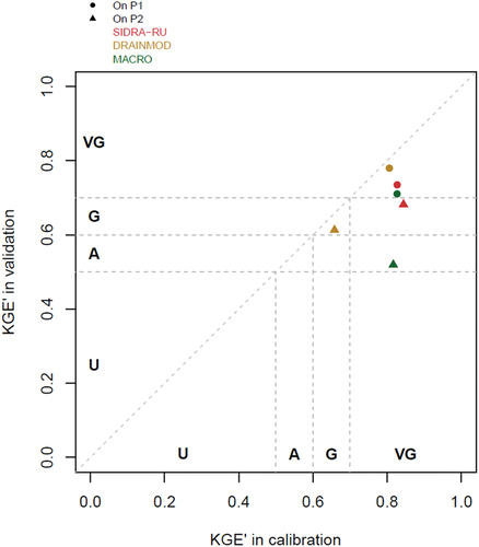
The calibrated parameters are available in Appendix A, Table A1. The models were calibrated against observed drainage discharge using the SAFRAN (for “Système d’Analyse Fournissant des Renseignements Adaptés à la Nivologie” in French) climate reanalysis (Vidal et al. 2010) as inputs over three periods – P1 (1999–2004), P2 (2005–2009), and P_tot (1999–2009) – thus providing three parameter sets (X1, X2, and X3) per hydrological model. These parameter sets were used thereafter to analyse the uncertainty stemming from the calibration procedure. Observed discharge data measured by the ARVALIS Institute, which monitors the La Jaillière site, were used. The three models achieved high performance, according to classic hydrological criteria such as the KGE’, Nash-Sutcliffe efficiency (NSE; Nash and Sutcliffe (1970)), root mean square error (RMSE; Chai and Draxler (2014)), and according to graphical diagnostics (see Appendix A, Fig. A1). The split-sample test (Klemeš 1986) highlighted that despite the aforementioned assumptions, the models were deemed temporally robust (see Appendix A, Fig. A2).

2.4 MC and climatic and hydrological indicators

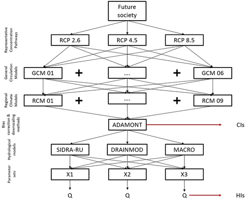
Once the hydrological models were calibrated, they were fed by CPs in order to simulate projected discharge series from 1975 to 2099. The MC is illustrated in Fig. 1; it comprises 30 CPs (Table 2) × 3 HMs × 3 parameter sets per HM (X_HMs) = 270 simulations. The uncertainty propagation was studied for both climate indicators (CIs) and HIs.

Figure 1. Modelling chain inducing the cascade of uncertainties.

The CIs were defined as seasonal volume of P and daily mean T, with a wet season (from October to March) and a dry season (from April to September). The subsurface drainage hydrology was studied according to four HIs:

• The dry season drained water balance (DDWB), i.e. the drained water volume flowing between 1 April and 30 September;

• The wet season drained water balance (WDWB), i.e. the drained water volume flowing between 1 October and 31 March. The DDWB and the WDWB are based on the annual drained water balance currently used in the literature (Pease et al. 2017, Mehan et al. 2019, Sojka et al. 2020, Golmohammadi et al. 2021, Jeantet et al. 2022);

• The length of the drainage season (LenDS; Jeantet et al. (2022)). The beginning of the drainage season is set to day d following Equation (1)(1) $\left\{\begin{array}{c}onthedayd:cumulativedischarge\ge Cu{m}_{Drainage}\\ \left[d+1:\hspace{0.17em}d+5\right]:cumulativedischarge\ge Cu{m}_{Drainage}+Cu{m}_{reliable}\end{array}\right\}$(1) :

(1) $\left\{\begin{array}{c}onthedayd:cumulativedischarge\ge Cu{m}_{Drainage}\\ \left[d+1:\hspace{0.17em}d+5\right]:cumulativedischarge\ge Cu{m}_{Drainage}+Cu{m}_{reliable}\end{array}\right\}$(1)

The $Cu{m}_{Drainage}$ threshold is set to 1.4 mm and the $Cu{m}_{reliable}$ to 2.7 mm (Henine et al. 2022), both corresponding to cumulative discharges from 1 August, defined as the beginning of the hydrological year. The end of the drainage season is set on the first day (d) when the difference between the annual drained water balance on 31 July, set as the end of the hydrological year, and the cumulative discharge at d is lower than the $Cu{m}_{Drainage}$ threshold (see Equation (2)(2) $onthedayd:Cu{m}_{total}-Cum\left[d\right]\ge Cu{m}_{Drainage}$(2) ):

(2) $onthedayd:Cu{m}_{total}-Cum\left[d\right]\ge Cu{m}_{Drainage}$(2)

Then, the duration of the drainage season is defined as the number of days between the start and the end of the drainage season:

• The discharge used to describe yearly high flow, i.e. a threshold defined as the 95^th percentile (Q_Q95) of daily discharge, a streamflow value not exceeded 5% of the time (Lemaitre-Basset et al. 2021).

2.5 Uncertainty analysis

In this study, we assessed six uncertainty sources: RCPs, GCMs, RCMs, HMs, X_HMs, and the climate internal variability. It was not possible to assess the uncertainty stemming from the bias correction and downscaling method because the ADAMONT method was the only one applied in the national dataset we used (Fig. 1). The QUALYPSO method (Evin et al. 2019), taken from the “QUALYPSO” R package (Evin 2020), was chosen to estimate the uncertainty ratio from the aforementioned sources. To obtain a robust estimation of uncertainty, the use of a complete multi-scenario MME of climate projections is a prerequisite (Sansom et al. 2013, Hingray and Saïd 2014, Evin et al. 2019) and, as described in section 2.2, the MME considered here was not complete. This problem was tackled with the QUALYPSO method, which uses a Bayesian data augmentation technique (Gelman and Rubin 1992) to fill in the matrix shown in Table 1 and to estimate the missing combinations by Bayesian inferences.

The QUALYPSO algorithm was then applied on the completed MME. First, the anomaly of the climate response from a given MC was simulated, i.e. each pathway from RCPs to hydrological simulations using only one model at each stage. Each MC was used to estimate the associated climatic and hydrological indicators. Then, the MC climate response was defined as the smoothing spline fitted to the 30-year rolling means of these raw indicators (see Appendix B, Equation (B1)(B1) $X\left(M{C}_i,t\right)=NFS\left(M{C}_i,t\right)+\eta \left(M{C}_i,t\right)$(B1) ). Eventually, the MC climate response could be described as an absolute or relative anomaly between a climate response over a historic control period (1975–2004) and a climate response over a future period (2006–2099). The internal variability variance of the MME was estimated as the mean value of the internal variability variances obtained for the different MCs (see Appendix B, Equation (B3)(B3) ${{\sigma }^2}_{int.var}=\frac{{\sum }_{i=1}^{n}var\left[X\left(M{C}_i\right)\right]}{n}$(B3) ).

Second, the uncertainty components of the MME were estimated by the ANOVA model, assuming that for a specific period the climate change response from a given MC might be the sum of the main effects of the different scenarios/models considered in the chain. In practical terms, each component of the MME induced its own effect, defined as the mean deviation of the component from the climate response of the given MC (Evin et al. 2019). This means that the uncertainty from an MME step, e.g. GCMs, was estimated as the variance of the dispersion between the mean climate change responses obtained for the different models of this step over all hydroclimatic combinations (see Equation (3)(3) $\$\begin{array}{rl}& {{\sigma }^2}_{tot}\left(y\right)={{\sigma }^2}_{RCP}\left(y\right)+{{\sigma }^2}_{GCM}\left(y\right)+{{\sigma }^2}_{RCM}\left(y\right)+{{\sigma }^2}_{HM}\left(y\right)\\ & +{{\sigma }^2}_{X_{HM}}\left(y\right)+{{\sigma }^2}_{int.var}\left(y\right)+{{\sigma }^2}_{res}\left(y\right)\end{array}$(3) ; Evin et al. (2019), Lemaitre-Basset et al. (2021)). Note that the ANOVA method in QUALYPSO assumes that the CP transient states are quasi-ergodic (QE-ANOVA), i.e. that for a given CP the statistical distribution over the whole period is similar to the one over an extracted sub-period (Hingray and Saïd 2014). Note also that a part of the total dispersion from the ANOVA decomposition cannot be explained by the additive uncertainty decomposition of each step of the MME. There is a residual variance, which cannot be attributed to a specific component of the MME.

(3) $\$\begin{array}{rl}& {{\sigma }^2}_{tot}\left(y\right)={{\sigma }^2}_{RCP}\left(y\right)+{{\sigma }^2}_{GCM}\left(y\right)+{{\sigma }^2}_{RCM}\left(y\right)+{{\sigma }^2}_{HM}\left(y\right)\\ & +{{\sigma }^2}_{X_{HM}}\left(y\right)+{{\sigma }^2}_{int.var}\left(y\right)+{{\sigma }^2}_{res}\left(y\right)\end{array}$(3)

With:

• ${{\sigma }^2}_{tot}$: the total variance in the year y;

• ${{\sigma }^2}_{RCP}$: the variance associated with RCPs;

• ${{\sigma }^2}_{GCM}$: the variance associated with GCMs;

• ${{\sigma }^2}_{RCM}$: the variance associated with RCMs;

• ${{\sigma }^2}_{HM}$: the variance associated with HMs;

• ${{\sigma }^2}_{X_{HM}}$: the variance associated with X_HMs;

• ${{\sigma }^2}_{int.var}$: the variance associated with internal variability;

• ${ }_{res}^2$: the residual variance.

3 Results

3.1 Uncertainty propagation in the CIs

Before analysing hydrological indicators, it is necessary to analyse the uncertainty propagation in climate indicators, as climate is the main driver of hydrological projections. Here, we analyse the wet season and dry season precipitation, as well as the wet season and dry season temperature.

The mean trends showed that the wet season (October–March) precipitation gradually increases in the future, up to +11% by 2085, i.e. +43 mm.6 months⁻¹ from ≈ 400 mm.6 months⁻¹ in the historical period (Fig. 2(a)). The wet season daily mean air temperature also gradually increases by up to +2.2°C, i.e. 9.5°C instead of 7.3°C in the historical period (Fig. 2(c)) by the end of the century. In both cases, the partitioning of uncertainty showed that before 2020, the main source of uncertainty is the climate internal variability, representing between 60% and 70% of the total uncertainty in 2000 (Fig. 2(b)–(d)). Then, the uncertainties of the two climate variables are mainly affected by GCMs and RCMs: from 40% to 65% of the total uncertainty for the wet season precipitation and from 50% to 70% for the wet season daily mean air temperature. The main difference between the partitioning of these two climate variables concerns RCPs. Regarding daily mean air temperature, RCPs represent up to 35% of the total uncertainty by 2060, while the RCP contribution to the uncertainty related to the wet season precipitation reaches 15% by 2080.

Figure 2. Mean trends in the spline fitted to the 30-year rolling mean of (a) wet season and (e) dry season precipitation (P) and of (c) wet season and (g) dry season daily mean air temperature (T). The mean trends are supported by 90% confidence intervals. The graphics in the bottom row ((b), (d), (f) and (h)) correspond to the partitioning of the total uncertainty, each one corresponding to the associated indicator in the graphics in the top row. “Res. Var.” refers to the residual variance and “Int. Variab” to the internal variability. Control period: 1975–2004.

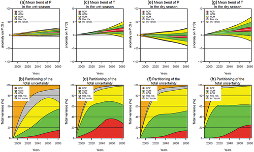
Moreover, results showed that the range of the dry season CIs was larger than the range of the wet season CIs. The mean trend of the dry season precipitation leads to a decrease of approximately 7% by 2080, i.e. −20 mm.6 months⁻¹ from ≈ 280 mm.6 months⁻¹ in the historical period (Fig. 2(e)). The dry season daily mean T increases by 2.6°C, i.e. 18.6°C instead of 16°C in the historical period, higher than the increase of the wet season T (Fig. 2(g)). Unlike for the wet season, the partitioning of uncertainty from the two climate variables is similar in the dry season (Fig. 2(f)–(h)), except for the slightly larger contribution of the RCPs to the daily mean T of approximately 10% by 2085. By 2085, the RCP contributions increase from 15% to 25%. In both cases, the GCMs and RCMs represent almost 80% of the total uncertainty in 2020. Specifically, the GCM contributions to the daily mean T are slightly larger than the contributions to the precipitation from 2050 by 10%, for both the dry and wet seasons. To sum up, the main sources of CI uncertainty are the GCMs and the RCMs, whose combined ratio accounted for at least half of the total uncertainty for all CIs from 2020.

3.2 Uncertainty propagation in the HIs

Here we analyse the WDWB and DDWB, as well as the LenDS and the 95^th percentile of daily discharge (Q_Q95). The mean trends showed that three HIs increase by the end of the 21^st century (Fig. 3(a)–(c), and (g)): by 19% for the WDWB (+25.7 mm.6 months⁻¹ from the historical 144 mm.6 months⁻¹); by +5% for the DDWB (+1.2 mm.6 months⁻¹ from the historical 24 mm.6 months⁻¹); and by 13% for the high flows (+0.32 mm.d⁻¹ from the historical 2.5 mm.d⁻¹). Conversely, the length of the drainage season decreases by 2% (4 days from the historical 156 days) by 2080 (Fig. 3(e)). The DDWD has the mean trend with the largest uncertainty range, with a relative anomaly from −100% to +100% (−20 mm.6 months⁻¹ to +20 mm.6 months⁻¹). The range for WDWB, LenDS, and Q_Q95 is smaller, from −40% to +60% depending on the HI considered.

Figure 3. Mean trends in the spline fitted to the 30-year rolling mean of (a) the WDWB, (c) the DDWB, (e) the LenDS, and (g) the Q_Q95. The graphics in the bottom row ((b), (d), (f) and (h)) represent the partitioning of the total uncertainty, each one corresponding to the associated indicator in the top row. The mean trends are supported by 90% confidence intervals. “Res. Var.” refers to the residual variance and “Int. Variab” to the internal variability. Control period: 1975–2004.

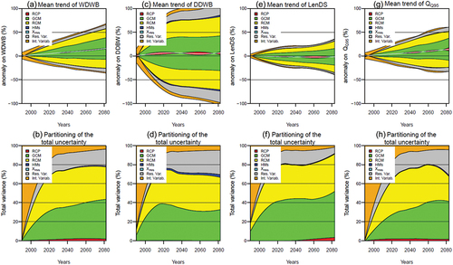
Similar to the CIs, the GCMs and the RCMs are the two main sources of uncertainty for the four HIs. The ratios for these two sources have almost identical values throughout the future period, with a cumulated ratio from 25% to 40% in 2000, gradually increasing to 70–90% by 2080 depending on the HI (Fig. (b), (d), (f), and (h)). Unlike the CIs, the RCP ratios are almost negligible for the four HIs, with a maximal partitioning of 5% for the LenDS by 2080. Moreover, the hydrological components of the MME also represent a negligible part of the total uncertainty for the four HIs. The HMs showed a maximal impact of 5% of the total uncertainty for the DDWB, and mean values ranged from 0.4% to 1.7% of the total uncertainty for the four HIs. The uncertainty ratios from the X_HMs are always close to 0%.

3.3 Main effects on CIs and HIs

Figure 4 shows the main effects of the RCPs, GCMs, RCMs, HMs, and X_HMs on the relative anomalies for the four HIs: WDWB, DDWB, LenDS, and Q_Q95. For each HI, the purpose is to highlight the specific effect of each component from the MME on the mean anomaly value of the HI in the projected future. For all HIs, the results showed that the members of the RCPs, HMs, and X_HMs do not diverge significantly from each other and that their contribution to the mean anomaly value is close to zero. The only minor exception concerns the effects of the HMs on the DDWB (Fig. 4 (i)): the SIDRA-RU and the MACRO models tend to reduce the DDWB by −11% and −1.5% by 2080, respectively, while the DRAINMOD model tends to increase the DDWB by +12.5% by 2080. The GCMs and the RCMs have the most divergent effects (Fig. 4 (b), (c), (g), (h), (l), (m), (q), and (r)), gradually increasing by the end of the century, and they have the largest effect on the DDWB: the values of the main effects by 2080 range from −30% to +40% and from −20% to +36% for the GCMs and the RCMs, respectively. Moreover, no specific GCM or RCM emerges with an effect distinguishing it from the rest that would be shared by all the HIs.

Figure 4. Main effects of the RCPs, GCMs, RCMs, HMs, and XHMs on the WDWB ((a), (b), (c), (d) and (e), respectively), the DDWB ((f), (g), (h), (i) and (j), respectively), the LenDS ((k), (l), (m), (n) and (o), respectively), and the Q_Q95 ((p), (q), (r), (s) and (t), respectively) projections. Solid lines represent the mean effect of each climate scenario or model; the 90% confidence interval of QUALYPSO estimations is drawn in shaded colour.

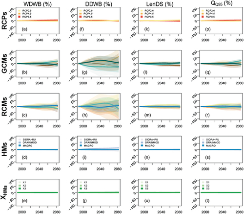
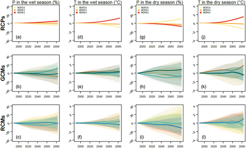
The same analyses were performed on the CIs (P and daily mean T in the wet and dry seasons) and are presented in Appendix C, Fig. C1. The results were quite similar to those observed for the HIs, as the GCMs and the RCMs are the two sources showing the largest deviations. The divergences between the RCP effects are larger for the CIs than they were for the HIs, specifically for the daily mean T. Similarly, the divergences from RCP effects are slightly larger for dry season CIs than for wet season CIs. However, the effect of the GCMs and the RCMs are still clearly dominant, which is consistent with the results presented in Fig. 2.

4 Discussion

4.1 Effects of the climate components of the MME on the total uncertainty

The distribution of the uncertainties is not constant over time for any HI or CI. The first source of uncertainty is the climate internal variability, ranging from 30% to 60% of the total uncertainty by 2005, until 2020 when it represents less than 20% of the uncertainty for all indicators. This dominant contribution varies according to the indicator studied (Hingray and Saïd 2014) and to the statistical post-treatment used for the studied indicator in the QUALYPSO method. Indeed, the use of 30-year rolling means on the indicators in this study instead of raw indicators explains the rapid decrease in the contribution of the internal variability after 2005 until finally falling below 10% by 2085 for almost all of the indicators (Vidal et al. 2016, Evin et al. 2019). This decreasing contribution also stems from the fact that the total uncertainty of all the indicators grows as the time approaches the year 2100, while the climate internal variability does not evolve significantly over the study period (Lafaysse et al. 2014).

The influence of RCPs varies depending on the variable. They show a low contribution to precipitation, not exceeding 15% in the entire period, while their contribution to the temperature reaches almost 40% by 2085, which is in agreement with the current literature (e.g. Khoi and Suetsugi 2012, Christensen and Kjellström 2020). The contribution of RCPs to the HI uncertainty is almost negligible compared to the GCM and RCM contributions. The lack of any influence of the RCPs on the Q_Q95 is quite surprising as they showed a significant contribution to the uncertainty of high flows in the literature (Vetter et al. 2017, Lemaitre-Basset et al. 2021). The difference from these studies might lie in the fact that we do not deal with conventional watershed hydrology in this paper. Comparing our results with subsurface drainage studies could be relevant; however, the few existing studies on subsurface drainage hydrology exploring uncertainty propagation in the MC did not differentiate between the climate components (e.g. Kujawa et al. 2020, Salla et al. 2021).

From 2020, the main sources of uncertainty for all the indicators are the GCMs and the RCMs, with similar contributions. Regarding the CIs, these contributions range from 50% to 90% of the total uncertainty, with the contributions being larger for precipitation. A direct consequence is the large range of CI anomalies, especially for dry season CIs. For instance, the future trend of dry season precipitation ranges from −40% to +25% by 2085, with 85% of the related uncertainty being covered by the cumulated GCM and RCM contributions. This result is congruent with previous studies, which showed that GCMs induce different seasonal precipitation responses to the projections, and RCMs add an additional layer of variability (Fowler et al. 2007, Jacob et al. 2014, Dayon et al. 2015, Tramblay and Somot 2018). Specifically, these results are rather consistent with the findings from Lemaitre-Basset et al. (2022), who also showed that GCMs and RCMs share the major part of uncertainty in PE projections over France, with a very similar dataset (no bias correction method was used by Lemaitre-Basset et al. (2022)), but the same GCM/RCM couples were used).

Regarding HIs, the results showed similar contributions from GCMs and RCMs, which were even larger: 70% to 90% of the total uncertainty from 2020 to 2085. This contribution is observed regardless of the specificities of each HI, whether cumulative such as the LenDS, DDWB, and WDWB or representative of the annual flow dynamics such as the Q_Q95, which is in agreement with the literature (Najafi et al. 2011, Habets et al. 2013, Vetter et al. 2015). The dry season indicator DDWB is impacted by the uncertainty related to the GCMs and the RCM, with anomalies ranging from −100% to +100% by 2085. Consequently, an anomaly from a particular year may be opposite to the mean trend despite this trend being deemed significant. This reveals an increasing variability in the drainage season subject to more extreme events that move it away from a typical average hydrological year. More harmful consequences for crops and an increased burden of management for farmers can be expected, especially in the dry season.

Despite being in agreement with the literature, the GCM and RCM contributions to HI uncertainty are exacerbated when compared with previous studies. The difference might be due to the low spatial scale in subsurface drainage compared with watershed hydrology. The La Jaillière site (0.01 km²) is included in one pixel from the CPs used (64 km²), and therefore P and PE data that feed the HMs were extracted from only one pixel, while the aforementioned studies on watershed hydrology used tens of pixels, e.g. ≈20 pixels in the study by Lemaitre-Basset et al. (2021). In an analysis not reported here, we assessed the impact of increasing the area of climatic influence around the study plot to 9 pixels and 25 pixels. The results of this analysis showed no difference in terms of the CI uncertainties from the QUALYPSO analysis, which lesd us to believe that the use of a single pixel had a low impact on our results and could not explain the over-representation of the GCMs and RCMs in the uncertainty share. Another factor explaining the low influence of RCPs might be that subsurface drainage hydrology is more seasonal than watershed hydrology, and is influenced more by precipitation than by air temperature. Therefore, similarly to precipitation, the HIs are more subject to the climate model uncertainty than to the uncertainty from the greenhouse gas emission scenarios.

4.2 Effects of the hydrological components of the MME on the total uncertainty

The current literature generally states that the hydrological components of an MME have almost no influence on the uncertainty related to mean and high flows in watershed hydrology (Christierson et al. 2012, Engin et al. 2017, Her et al. 2019, Kujawa et al. 2020, Lemaitre-Basset et al. 2021, Salla et al. 2021). Similar conclusions can be drawn for the WDWB, the LenDS and Q_Q95 indicators, i.e. indicators that mainly depend on flows in the wet season. This reassures us of the accuracy of the assumptions made concerning the hydrological models (see section 2.3): neglecting current crops, neglecting surface runoff, and simplifying the soil profile description in both the DRAINMOD and MACRO models.

However, the literature also states that the contributions of HMs and X_HMs to the total uncertainty in low flows are less negligible (Habets et al. 2013, Engin et al. 2017, Vetter et al. 2017, Dallaire et al. 2021), which is not in agreement with our results. We showed that hydrological modelling has a contribution not exceeding 5% to the DDWB, the indicator that describes low flows in our study. The aforementioned studies generally established their results on temporal dynamic indicators such as the MAM7, i.e. the mean-annual minimal discharge during seven consecutive days (Lemaitre-Basset et al. 2021), or the annual Q_Q10 (discharge not exceeded 10% of the time; Vetter et al. (2017)), whereas the DDWB is a cumulative indicator, thus making the comparison with the current literature less adequate. The seasonal aspect of drainage hydrology makes the use of these conventional hydrological indicators unsuitable because low flows mainly appear in summer when subsurface drainage is often null or marked by very episodic events. Other indicators must be used to describe the temporal aspect of subsurface drainage such as the length of the drainage or the length of the period with no flow (Jeantet et al. 2022).

Overall, this study shows that HMs do not significantly influence the total uncertainty. However, this statement is restricted by: (1) the fact that the QUALYPSO method establishes the contribution of each source from the MME relative to the others, and thus if GCM, or RCM, contributions are too significant, the HM effects are reduced; (2) the choice of the HIs, as highlighted above. The last point is supported by Fig. 5, which shows a comparison of the flow-duration curve (FDC) between observations and simulations obtained using the SAFRAN database during the calibration process (FDC_REF) (a) and the simulations obtained from the CPs of the MME (FDC_{CP_MME}) (b). For a specific HM, the FDC_{CP_MME}(i) from each MC i corresponding to the HM was calculated from the non-null discharges of the MC i. Then, a unique FDC_{CP_MME} per HM was extracted from the median of these FDC_{CP_MME}. The analyses were conducted for the period 1999–2009, corresponding to the availability of the observed data for the Jaillière site (Henine et al. 2022).

Figure 5. Comparison of (a) flow-duration curves on a logarithmic scale for drainage observations and calibrated simulation and (b) simulations from all the modelling chains of the MME, over the calibration period (1999–2009). In all cases, only the non-null discharges are considered. Per HM (SIDRA-RU, DRAINMOD, MACRO), the curve from the MME (b) was calculated as the median of frequencies from each chain i. A 90% confidence interval was defined from the 5^th to 95^th quantiles.

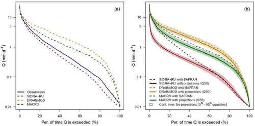
The results show that regarding FDC_REF (Fig. 5(a)) the SIDRA-RU model is the closest to the observations on the high, average, and low flows, while MACRO and DRAINMOD overestimate the average and low flows. These results are consistent with the performance from the calibration process (see section 2.3.4 and Appendix A). However, the use of CPs in SIDRA-RU instead of observed climate (SAFRAN) changes the FDC, especially for discharges above 1 mm.d⁻¹ while the use of CPs in the DRAINMOD and MACRO models affects their FDCs less (Fig. 5(b)). This result is surprising as the HM effects on high flows are null (see Q_Q95 on Fig. 4(s)). In low flows, the use of CPs does not affect the FDC of any model compared to SAFRAN. All these results highlight the fact that even if the climate models induce most of the uncertainties, the choice of the HM is crucial especially when only one is involved. Indeed, the choice of model is restricted to the needs of the study and therefore not all models are equal.

4.3 Limitations of the study

Another point to be discussed deals with the dependency of the aforementioned interpretations on the methodological choices and data involved in this study. First, the methodological choices made for both the DRAINMOD and MACRO models (section 2.3.4) were efficient regarding the HIs we studied, but they certainly might not be relevant if the HIs change. The DRAINMOD and MACRO models showed a slightly weaker performance than the SIDRA-RU, specifically for low flows (section 4.2). This might be due to the fact that crop rotation was neglected, whereas it plays a significant role in the calculation of the actual evapotranspiration (AE) from PE in these two models (Larsbo et al. 2005, Skaggs et al. 2012). The assumption neglecting the current crops is suitable only in the conditions defined in this study.

Second, the ADAMONT method was the only downscaling and bias correction method used to process data from RCMs to the spatial resolution used (see section 2.2). However, it is known that this step contributes significantly to the total uncertainty (Hingray and Saïd 2014, Lafaysse et al. 2014). Using several downscaling and bias correction methods could improve the partitioning of uncertainty of this study. In the national Drias 2020 dataset used here, only one downscaling and bias correction method was available at the time of the study.

Finally, the ANOVA from the QUALYPSO method may introduce some limitations in the analyses, especially on relative anomalies from hydrological extremes such as the Q_Q95 used here, “with the hypotheses not verified as the normal distribution and the homoscedasticity of residuals” (Lemaitre-Basset et al. 2021, p. 13). One way to fix this issue could be to use absolute anomalies instead of relative ones for hydrological extremes.

5 Conclusions

The aim of this study was to assess the uncertainty propagation in an MME simulating the future of subsurface drainage hydrology under climate change on a site representative of French subsurface drainage. The results showed that the anomalies of the study indicators vary, and are larger for indicators specific to the dry season, e.g. the drained water balance. The results also showed that, from 2020 and regarding CIs and HIs alike, GCMs and RCMs are the two main sources of uncertainty in the MME, with cumulated contributions ranging from 50% to 90% from 2020 to 2085. Despite having almost no influence on the HIs, the influence of the RCPs on the CIs reaches 40% for the dry season temperature by 2085 but does not exceed 15% for wet season precipitation. Furthermore, the hydrological models show almost no influence on the total uncertainty for any HIs, nor do their parameters, despite the strong assumptions made about their functional structure. Finally, this last point established that, true to its purpose, the SIDRA-RU model could confidently be used for the prediction of subsurface drainage discharge under climate change. However, we based our conclusions on four HIs to describe subsurface drainage hydrology. One way to generalize the conclusions of the study would be to use a more complete panel of HIs to better describe the uncertainty propagation in all aspects of subsurface drainage. Using the CPs from the new CMIP6 project, which is not yet available (i.e. regionalized) for local hydrological purposes, could also be interesting for evaluating the dependency of this study on the climate projections used, with the potential aim of decreasing the contribution of climate models to the total uncertainty.

Software availability statement

The “QUALYPSO” package (Evin 2020) and the “airGR” package (Coron et al. 2017, 2020) are both R packages freely available on the R CRAN repository. An intellectual property certificate has been issued by the Agency for Program Protection for the SIDRA-RU model code, under the reference IDDN.FR.001.260018.000.S.P.2018.000.30100. There is no public repository providing it. However, Jeantet et al. (2021) and Henine et al. (2022) provide an exhaustive description of the model, enabling readers to easily reproduce it. The code is written in FORTRAN language. The MACRO model execution program is freely available via the portal of the Swedish University of Agricultural Sciences (https://www.slu.se/en/). The DRAINMOD model execution program is freely available via the portal of the North Carolina State University (https://www.bae.ncsu.edu/agricultural-water-management). The three models SIDRA-RU, MACRO and DRAINMOD were imported in R software to be computed with the calibration algorithm “airGR.”

Acknowledgements

We express our gratitude to the Météo-France Meteorological Agency for providing the SAFRAN data and the climate projections from the Euro-Cordex CMIP5 project used in this work. Moreover, we thank the ARVALIS Institute for providing data from the La Jaillière measurement site. We thank Lila Collet, who processed the Euro-Cordex CMIP5 project data to make them usable for this study. We also thank Mohamed Youssef for providing us guidelines on the DRAINMOD model. Finally, we thank Guillaume Evin for his very useful advice on using the QUALYPSO method.

Disclosure statement

No potential conflict of interest was reported by the authors.

Data availability statement

Observed climatic data (SAFRAN) for this work were provided by Météo-France and are not publicly available since they are part of a commercial product. Météo-France can freely provide them on request for research and non-profit purposes. Projection climatic data are available via the Drias web portal (http://www.drias-climat.fr/).

Additional information

Funding

This research was supported by the Agence Nationale de la Recherche under the “Investissements d’avenir” programme [grant no. ANR-16-CONV-0003; CLAND project].

Appendix Appendix A

Equations used in both the DRAINMOD and MACRO models for the hydrological component:

• The Van Genuchten equations (Van Genuchten 1980):

(A1) $\theta \left(h\right)={\theta }_r+\frac{{\theta }_s-{\theta }_r}{{\left[1+{\left|\alpha h\right|}^n\right]}^{1-\frac{1}{n}}}$(A1)

(A2) $K\left(h\right)=K_{sat}\ast {\left(\frac{\theta \left(h\right)-{\theta }_r}{{\theta }_s-{\theta }_r}\right)}^{\frac{1}{2}}\ast {\left[1-{\left(1-{\left(\frac{\theta \left(h\right)-{\theta }_r}{{\theta }_s-{\theta }_r}\right)}^{\frac{n}{n-1}}\right)}^{1-\frac{1}{n}}\right]}^2$(A2)

• The Green-Ampt equation (Green and Ampt 1911):

(A3) $f=K_{sat}+\frac{K_{sat}\ast M\ast S_{av}}{F}=\frac{A}{F}+B$(A3)

• The relations between upward flux, water table, and drained water volume (Skaggs 1981):

(A4) $V_d={\int }_0^{y_1}\left({\theta }_0\left(y\right)-\theta \left(y\right)\right)dy$(A4)

(A5) $q\left(h\right)=-K\left(h\right)\frac{dh}{dz}+K\left(h\right)$(A5)

With:

• $h$: water pressure (cm);

• $\theta \left(h\right)$: water content at $h$ (-);

• ${\theta }_r$: residual water content (-);

• ${\theta }_s$: saturation water content (-);

• $\alpha$: Van Genuchten parameter (cm⁻¹);

• $n$: Van Genuchten parameter (-);

• $K\left(h\right)$: hydraulic conductivity at $h$ (cm.h⁻¹);

• $K_{sat}$: saturation hydraulic conductivity (cm.h⁻¹);

• $f$: infiltration (cm.h⁻¹);

• $M$: available water content, i.e. difference between ${\theta }_s$ and the initial water content ${\theta }_i$ (-);

• $S_{av}$: suction head (cm);

• $F$: cumulated infiltration (cm);

• $A$ and $B$: Green-Ampt parameters, dependent on soil properties, ${\theta }_i$ and surface conditions;

• $V_d$: drained water volume per surface unit (cm.h⁻¹);

• ${\theta }_0\approx {\theta }_s$: water content before drainage (-);

• $y_1$: water table depth (cm);

• $q\left(h\right)$: upward flux per surface unit (cm.h⁻¹);

• $z$: location on the soil profile (cm).

  Table A1. Model parameters of SIDRA-RU, DRAINMOD, and MACRO calibrated on three periods: P1 (1999–2004), P2 (2005–2009), and on the total calibration period P_tot (1999–2009).

  Model	Time period	Soil layer	$n$(-)	$\alpha$ (cm^−1)	${\theta }_s$ (%)	${\theta }_r$ (%)	$K_{sat}$(m.d^−1)	µ(-)	$S_{inter}$ (mm)	$S_{max}$ (mm)
  SIDRA-RU	P1	-	-	-	-	-	0.5	0.0	98.7	120.0
  	P2	-	-	-	-	-	0.3	0.0	155.7	160.7
  	Ptot	-	-	-	-	-	0.4	0.0	123.0	132.0
  DRAINMOD	P1	Top	1.5	0.0	50.0	0.0	0.4	-	-	-
  		Bottom	1.5	0.0	41.6	0.0	4.8	-	-	-
  	P2	Top	1.1	0.0	47.8	0.0	0.6	-	-	-
  		Bottom	1.2	0.0	55.0	0.0	5.1	-	-	-
  	Ptot	Top	1.1	0.0	48.7	0.0	1.6	-	-	-
  		Bottom	1.2	0.0	43.8	0.0	4.9	-	-	-
  MACRO	P1	-	1.1	0.0	35.6	0.0	1.7	-	-	-
  	P2	-	1.1	0.0	35.5	0.0	0.8	-	-	-
  	Ptot	-	1.1	0.0	35.7	0.0	2.0	-	-	-

Figure A1. Graphical and numerical evaluation of the three hydrological models over the complete calibration period (1999–2009).

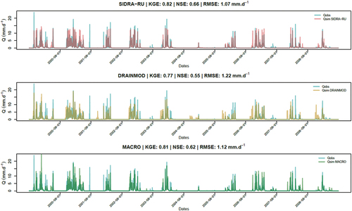
Figure A2. Results from the split-sample test on the three hydrological models for the periods P1 (1999–2004) and P2 (2005–2009). The letters U (unsatisfying), A (acceptable), G (good), and VG (very good) categorize the KGE’ values (Jeantet et al. 2021).

Appendix B

Equations used in the QUALYPSO method to estimate the climate change response $X$, its anomaly over the future period, and its variance (Hingray and Saïd 2014):

(B1) $X\left(M{C}_i,t\right)=NFS\left(M{C}_i,t\right)+\eta \left(M{C}_i,t\right)$(B1)

(B2) $var\left[X\left(M{C}_i\right)\right]=\left[NFS\left(M{C}_i\right)\right]+\left[\eta \left(M{C}_i\right)\right]$(B2)

(B3) ${{\sigma }^2}_{int.var}=\frac{{\sum }_{i=1}^{n}var\left[X\left(M{C}_i\right)\right]}{n}$(B3)

(B4) $\widehat{NFS\left(M{C}_i,t\right)}=NFS\left(M{C}_i,t\right)-NFS\left(M{C}_i,c\right)$(B4)

(B5) $\widehat{NFS\left(M{C}_i,t\right)}=\frac{NFS\left(M{C}_i,t\right)}{NFS\left(M{C}_i,c\right)}-1$(B5)

With:

• $X$: the climate response at the time t from the modelling chain $M{C}_i$;

• $NFS$: the noise-free signal, i.e. the desired value at time t, assuming the signal of the $M{C}_i$ is quasi-ergodic (Hingray and Saïd 2014);

• $\eta$: the residue at time t;

• $n$: the number of modelling chains in the MME, i.e. $n=270$;

• ${{\sigma }^2}_{int.var}$: the climate internal variability variance;

• $\widehat{NFS}$: absolute (Equation (C4)) or relative (Equation (C5)) anomaly a climate response over a control period c and a future period t;

Appendix C

Figure C1. Main effects of RCPs, GCMs, and RCMs on the precipitation projections (a, b, c) and on the daily mean air temperature projections (d, e, f) in the wet season, respectively, and on the precipitation projections (g, h, i) and on the daily mean air temperature projections (j, k, l) in the dry season, respectively. Solid lines represent the mean effect of each climate scenario or model; the 90% confidence interval of QUALYPSO estimations is drawn in shaded colour.

References

- Abd-Elaty, I., et al., 2019. Effects of climate change on the design of subsurface drainage systems in coastal aquifers in arid/semi-arid regions: case study of the Nile delta. Science of the Total Environment, 672, 283–295. doi:10.1016/j.scitotenv.2019.03.483.
- Addor, N., et al., 2014. Robust changes and sources of uncertainty in the projected hydrological regimes of Swiss catchments. Water Resources Research, 50 (10), 7541–7562. doi:10.1002/2014WR015549.
- Adriaanse, P., et al., 1996. Surface water models and EU registration of plant protection products. IRSTEA. Available from: https://esdac.jrc.ec.europa.eu/public_path/projects_data/focus/docs/sw_en_6476VI96_24Feb1997.pdf [Accessed 22 November 2022].
- Alaoui, A., et al., 2003. Dual-porosity and kinematic wave approaches to assess the degree of preferential flow in an unsaturated soil. Hydrological Sciences Journal, 48 (3), 455–472. doi:10.1623/hysj.48.3.455.45289.
- Arnell, N.W. and Gosling, S.N., 2016. The impacts of climate change on river flood risk at the global scale. Climatic Change, 134 (3), 387–401. doi:10.1007/s10584-014-1084-5.
- Baize, D. and Jabiol, B., 2011. Guide pour la description des sols. Editions Quae. Available from: https://hal.archives-ouvertes.fr/hal-01195043 [Accessed 15 November 2022].
- Beulke, S., Brown, C.D., Jarvis, N.J., 2001. Macro: a preferential flow model to simulate pesticide leaching and movement to drains, and J.B.H.J. Linders, ed. Modelling of environmental chemical exposure and risk. Dordrecht: Springer Netherlands, 117–132. doi:10.1007/978-94-010-0884-6_12.
- Boussinesq, J., 1904. Recherches théoriques sur l’écoulement des nappes d’eau infiltrées dans le sol et sur le débit des sources. Journal de Mathématiques Pures et Appliquées, 10, 5–78.
- Brown, R.A., Skaggs, R.W., and Hunt, W.F., 2013. Calibration and validation of DRAINMOD to model bioretention hydrology. Journal of Hydrology, 486, 430–442. doi:10.1016/j.jhydrol.2013.02.017.
- Chai, T. and Draxler, R.R., 2014. Root mean square error (RMSE) or mean absolute error (MAE)? – arguments against avoiding RMSE in the literature. Geoscientific Model Development, 7 (3), 1247–1250. doi:10.5194/gmd-7-1247-2014.
- Christensen, O.B. and Kjellström, E., 2020. Partitioning uncertainty components of mean climate and climate change in a large ensemble of European regional climate model projections. Climate Dynamics, 54 (9), 4293–4308. doi:10.1007/s00382-020-05229-y.
- Christierson, B.V., Vidal, J.-P., and Wade, S.D., 2012. Using UKCP09 probabilistic climate information for UK water resource planning. Journal of Hydrology, 424–425, 48–67. doi:10.1016/j.jhydrol.2011.12.020.
- Córdova, M., et al., 2015. Evaluation of the penman-monteith (FAO 56 PM) method for calculating reference evapotranspiration using limited data. Mountain Research and Development, 35 (3), 230–239. doi:10.1659/MRD-JOURNAL-D-14-0024.1.
- Coron, L., et al., 2017. The suite of lumped GR hydrological models in an R package. Environmental Modelling and Software, 94, 166–171. doi:10.1016/j.envsoft.2017.05.002.
- Coron, L., et al., 2020. airGR: suite of GR hydrological models for precipitation-runoff modelling. R package version 1.4.3.65. doi:10.15454/EX11NA.
- Dairon, R., 2015. Identification des processus dominants de transfert des produits phytosanitaires dans le sol et évaluation de modèles numériques pour des contextes agro-pédo-climatiques variés. Lyon 1. Lyon.
- Dairon, R., et al., 2017. Long-term impact of reduced tillage on water and pesticide flow in a drained context. Environmental Science and Pollution Research, 24 (8), 6866–6877. doi:10.1007/s11356-016-8123-x.
- Dallaire, G., et al., 2021. Uncertainty of potential evapotranspiration modelling in climate change impact studies on low flows in North America. Hydrological Sciences Journal, 66 (4), 689–702. doi:10.1080/02626667.2021.1888955.
- Dayon, G., Boé, J., and Martin, E., 2015. Transferability in the future climate of a statistical downscaling method for precipitation in France. Journal of Geophysical Research: Atmospheres, 120 (3), 1023–1043. doi:10.1002/2014JD022236.
- Dayyani, S., et al., 2012. Impact of climate change on the hydrology and nitrogen pollution in a tile-drained agricultural watershed in eastern Canada. Transactions of the ASABE, 55, 389–401. doi:10.13031/2013.41380.
- Deelstra, J., 2015. Climate change and subsurface drainage design: results from a small field-scale catchment in south-western Norway. Acta Agriculturae Scandinavica, Section B — Soil & Plant Science, 65 (sup1), 58–65. doi:10.1080/09064710.2014.975836.
- Deser, C., et al., 2012. Uncertainty in climate change projections: the role of internal variability. Climate Dynamics, 38 (3), 527–546. doi:10.1007/s00382-010-0977-x.
- Engin, B.E., Yücel, I., and Yilmaz, A., 2017. Assessing different sources of uncertainty in hydrological projections of high and low flows: case study for Omerli Basin, Istanbul, Turkey. Environmental Monitoring and Assessment, 189 (7), 347. doi:10.1007/s10661-017-6059-3.
- Evin, G., et al., 2019. Partitioning uncertainty components of an incomplete ensemble of climate projections using data augmentation. Journal of Climate, 32 (8), 2423–2440. doi:10.1175/JCLI-D-18-0606.1.
- Evin, G., 2020. QUALYPSO: partitioning uncertainty components of an incomplete ensemble of climate projections. R package version 1.2. Available from: https://CRAN.R-project.org/package=QUALYPSO [Accessed 14 June 2023].
- FOCUS., 2012. FOCUS surface water scenarios in the EU evaluation process under 91/414/EEC. Report of the FOCUS Working Group on Surface Water Scenarios. EC Document Reference SANCO/4802/2001-rev.2 (Revised version SANCO/4802/2001-rev.2). FOCUS, p. 245.
- Fowler, H.J., et al., 2007. Estimating change in extreme European precipitation using a multimodel ensemble. Journal of Geophysical Research: Atmospheres, 112, D18. doi:10.1029/2007JD008619.
- Garner, G., et al., 2015. Hydroclimatology of extreme river flows. Freshwater Biology, 60 (12), 2461–2476. doi:10.1111/fwb.12667.
- Gelman, A. and Rubin, D.B., 1992. Inference from iterative simulation using multiple sequences. Statistical Science, 7 (4), 457–472. doi:10.1214/ss/1177011136.
- Golmohammadi, G., et al., 2021. Assessment of impacts of climate change on tile discharge and nitrogen yield using the DRAINMOD Model. Hydrology, 8 (1), 1. doi:10.3390/hydrology8010001.
- Green, H. and Ampt, G.A., 1911. Studies on soil physics: part I. The Journal of Agricultural Science, 4 (1), 1–24. doi:10.1017/S0021859600001441.
- Grusson, Y., Wesström, I., and Joel, A., 2021. Impact of climate change on Swedish agriculture: growing season rain deficit and irrigation need. Agricultural Water Management, 251, 106858. doi:10.1016/j.agwat.2021.106858.
- Gupta, H.V., et al., 2009. Decomposition of the mean squared error and NSE performance criteria: implications for improving hydrological modelling. Journal of Hydrology, 377 (1), 80–91. doi:10.1016/j.jhydrol.2009.08.003.
- Habets, F., et al., 2013. Impact of climate change on the hydrogeology of two basins in northern France. Climatic Change, 121 (4), 771–785. doi:10.1007/s10584-013-0934-x.
- Hawkins, E. and Sutton, R., 2009. The potential to narrow uncertainty in regional climate predictions. Bulletin of the American Meteorological Society, 90 (8), 1095–1108. doi:10.1175/2009BAMS2607.1.
- Hawkins, E. and Sutton, R., 2011. The potential to narrow uncertainty in projections of regional precipitation change. Climate Dynamics, 37 (1), 407–418. doi:10.1007/s00382-010-0810-6.
- Henine, H., et al., 2022. Coupling of a subsurface drainage model with a soil reservoir model to simulate drainage discharge and drain flow start. Agricultural Water Management, 262, 107318. doi:10.1016/j.agwat.2021.107318.
- Henine, H., Nédélec, Y., and Ribstein, P., 2014. Coupled modelling of the effect of overpressure on water discharge in a tile drainage system. Journal of Hydrology, 511, 39–48. doi:10.1016/j.jhydrol.2013.12.016.
- Her, Y., et al., 2019. Uncertainty in hydrological analysis of climate change: multi-parameter vs. multi-GCM ensemble predictions. Scientific Reports, 9 (1), 4974. doi:10.1038/s41598-019-41334-7.
- Hingray, B., et al., 2019. Uncertainty component estimates in transient climate projections. Climate Dynamics, 53 (5), 2501–2516. doi:10.1007/s00382-019-04635-1.
- Hingray, B. and Saïd, M., 2014. Partitioning internal variability and model uncertainty components in a multimember multimodel ensemble of climate projections. Journal of Climate, 27 (17), 6779–6798. doi:10.1175/JCLI-D-13-00629.1.
- Hooghoudt, S.B., 1940. General consideration of the problem of field drainage by parallel drains, ditches, watercourses, and channels. In: Contribution to the knowledge of some physical parameters of the soil, Bodemkundig Instituut, Groningen, Netherlands, 7.
- ICID, 2021. Agricultural water management for sustainable rural development (Annual report). New Dehli, India: ICID, p. 92.
- IPCC, 2014. Climate change 2014: impacts, adaptation, and vulnerability. Part A: global and sectoral aspects. Contribution of working group II to the fifth assessment report of the intergovernmental panel on climate change, R.K. Pachauri and L.A. Meyer, eds. Cambridge University Press.
- IPCC, 2021. Climate change 2021: the physical science basis. Contribution of working group I to the sixth assessment report of the intergovernmental panel on climate change. V. Masson-Delmotte, et al., eds. Cambridge University Press.
- Jacob, D., et al., 2014. EURO-CORDEX: new high-resolution climate change projections for European impact research. Regional Environmental Change, 14 (2), 563–578. doi:10.1007/s10113-013-0499-2.
- Jamagne, M., 1968. Bases et techniques d’une cartographie des sols. Vol. 18. Paris: Institut National de la Recherche Agronomique. Available from: https://www.persee.fr/doc/geo_0003-4010_1969_num_78_428_15899 [Accessed 15 November 2022].
- Jarvis, N.J., et al., 1997. MACRO—DB: a decision-support tool for assessing pesticide fate and mobility in soils. Environmental Modelling & Software, 12 (2), 251–265. doi:10.1016/S1364-8152(97)00147-3.
- Jeantet, A., et al., 2021. Robustness of a parsimonious subsurface drainage model at the French national scale. Hydrology and Earth System Sciences, 25 (10), 5447–5471. doi:10.5194/hess-25-5447-2021.
- Jeantet, A., et al., 2022. Effects of climate change on hydrological indicators of subsurface drainage for a representative french drainage site. Frontiers in Environmental Science, 10. doi:10.3389/fenvs.2022.899226.
- Jiang, Q., et al., 2020. Assessing climate change impacts on greenhouse gas emissions, N losses in drainage and crop production in a subsurface drained field. Science of the Total Environment, 705, 135969. doi:10.1016/j.scitotenv.2019.135969.
- Khaliq, M.N., et al., 2009. Identification of hydrological trends in the presence of serial and cross correlations: a review of selected methods and their application to annual flow regimes of Canadian rivers. Journal of Hydrology, 368 (1), 117–130. doi:10.1016/j.jhydrol.2009.01.035.
- Khoi, D.N. and Suetsugi, T., 2012. Uncertainty in climate change impacts on streamflow in be river catchment, Vietnam. Water and Environment Journal, 26 (4), 530–539. doi:10.1111/j.1747-6593.2012.00314.x.
- Klemeš, V., 1986. Operational testing of hydrological simulation models. Hydrological Sciences Journal, 31 (1), 13–24. doi:10.1080/02626668609491024.
- Kling, H., Fuchs, M., and Paulin, M., 2012. Runoff conditions in the upper Danube basin under an ensemble of climate change scenarios. Journal of Hydrology, 424–425, 264–277. doi:10.1016/j.jhydrol.2012.01.011.
- Konyha, D. and Skaggs, R.W., 1992. A coupled, field hydrology – open channel flow model: theory. Transactions of the ASAE, 35 (5), 1431–1440. doi:10.13031/2013.28750.
- Kujawa, H., et al., 2020. The hydrologic model as a source of nutrient loading uncertainty in a future climate. Science of the Total Environment, 724, 138004. doi:10.1016/j.scitotenv.2020.138004.
- Kundzewick, Z.W., et al., 2008. The implications of projected climate change for freshwater resources and their management. Hydrological Sciences Journal, 53 (1), 3–10. doi:10.1623/hysj.53.1.3.
- Kundzewicz, Z.W., et al., 2014. Flood risk and climate change: global and regional perspectives. Hydrological Sciences Journal, 59 (1), 1–28. doi:10.1080/02626667.2013.857411.
- Kuzmanovski, V., et al., 2015. Modeling water outflow from tile-drained agricultural fields. Science of the Total Environment, 505, 390–401. doi:10.1016/j.scitotenv.2014.10.009.
- Lafaysse, M., et al., 2014. Internal variability and model uncertainty components in future hydrometeorological projections: the Alpine Durance basin. Water Resources Research, 50 (4), 3317–3341. doi:10.1002/2013WR014897.
- Lagacherie, P. and Favrot, J.C., 1987. Synthèse générale sur les études de secteurs de référence drainage. Paris, France: INRA.
- Lange, B., Germann, P.F., and Lüscher, P., 2011. Runoff-generating processes in hydromorphic soils on a plot scale: free gravity-driven versus pressure-controlled flow. Hydrological Processes, 25 (6), 873–885.
- Larsbo, M., et al., 2005. An improved dual-permeability model of water flow and solute transport in the vadose zone. Vadose Zone Journal, 4 (2), 398–406. doi:10.2136/vzj2004.0137.
- Larsbo, M. and Jarvis, N.J., 2003. MACRO 5.0. A model of water flow and solute transport in macroporous soil (Technical report). Uppsala, SWEDEN: Swedish University of Agricultural Sciences, p. 52.
- Lebrun, J.D., et al., 2019. Ecodynamics and bioavailability of metal contaminants in a constructed wetland within an agricultural drained catchment. Ecological Engineering, 136, 108–117. doi:10.1016/j.ecoleng.2019.06.012.
- Lemaitre-Basset, T., et al., 2021. Climate change impact and uncertainty analysis on hydrological extremes in a French Mediterranean catchment. Hydrological Sciences Journal, 66 (5), 888–903. doi:10.1080/02626667.2021.1895437.
- Lemaitre-Basset, T., et al., 2022. Unraveling the contribution of potential evaporation formulation to uncertainty under climate change. Hydrology and Earth System Sciences, 26 (8), 2147–2159. doi:10.5194/hess-26-2147-2022.
- Liang, X.-Z., et al., 2008. Regional climate models downscaling analysis of general circulation models present climate biases propagation into future change projections. Geophysical Research Letters, 35, 8. doi:10.1029/2007GL032849.
- Maurer, E.P., et al., 2010. The utility of daily large-scale climate data in the assessment of climate change impacts on daily streamflow in California. Hydrology and Earth System Sciences, 14 (6), 1125–1138. doi:10.5194/hess-14-1125-2010.
- Mechoso, C.R. and Arakawa, A., 2003. GENERAL CIRCULATION | models, and J.R. Holton, ed. Encyclopedia of atmospheric sciences. Oxford: Academic Press, 861–869. doi:10.1016/B0-12-227090-8/00157-3.
- Mehan, S., et al., 2019. Assessment of hydrology and nutrient losses in a changing climate in a subsurface-drained watershed. Science of the Total Environment, 688, 1236–1251. doi:10.1016/j.scitotenv.2019.06.314.
- Micheli, E., et al., 2006. World reference base for soil resources: 2006: a framework for international classification, correlation and communication. Rome, Italy: FAO.
- Moeys, J., et al., 2009. Functional test of FOOTPRINT pedotransfer functions for the dual-permeability model MACRO. In EGU General Assembly Conference Abstracts. Vienna, Austria, 7237.
- Moeys, J., et al., 2012. Functional test of pedotransfer functions to predict water flow and solute transport with the dual-permeability model MACRO. Hydrology and Earth System Sciences, 16 (7), 2069–2083.
- Najafi, M.R., Moradkhani, H., and Jung, I.W., 2011. Assessing the uncertainties of hydrologic model selection in climate change impact studies. Hydrological Processes, 25 (18), 2814–2826. doi:10.1002/hyp.8043.
- Nash, J.E. and Sutcliffe, J.V., 1970. River flow forecasting through conceptual models part I — a discussion of principles. Journal of Hydrology, 10 (3), 282–290. doi:10.1016/0022-1694(70)90255-6.
- Navarro-Racines, C., et al., 2020. High-resolution and bias-corrected CMIP5 projections for climate change impact assessments. Scientific Data, 7 (1), 7. doi:10.1038/s41597-019-0343-8.
- Northrop, P.J. and Chandler, R.E., 2014. Quantifying sources of uncertainty in projections of future climate. Journal of Climate, 27 (23), 8793–8808. doi:10.1175/JCLI-D-14-00265.1.
- Parajka, J., et al., 2016. Uncertainty contributions to low-flow projections in Austria. Hydrology and Earth System Sciences, 20 (5), 2085–2101. doi:10.5194/hess-20-2085-2016.
- Pease, L.A., et al., 2017. Projected climate change effects on subsurface drainage and the performance of controlled drainage in the western Lake Erie Basin. Journal of Soil and Water Conservation, 72 (3), 240–250. doi:10.3390/agronomy10050625.
- Phillips, N.A., 1956. The general circulation of the atmosphere: a numerical experiment. Quarterly Journal of the Royal Meteorological Society, 82 (352), 123–164. doi:10.1002/qj.49708235202.
- Potter, N.J., et al., 2020. Bias in dynamically downscaled rainfall characteristics for hydroclimatic projections. Hydrology and Earth System Sciences, 24 (6), 2963–2979. doi:10.5194/hess-24-2963-2020.
- Prudhomme, C., et al., 2014. Hydrological droughts in the 21st century, hotspots and uncertainties from a global multimodel ensemble experiment. Proceedings of the National Academy of Sciences, 111(9), 3262–3267. doi:10.1073/pnas.1222473110.
- Randall, D.A., Editor, & Zehnder, J., Reviewer. (2001). General circulation model development: past, present, and future. International Geophysics Series, Vol 70. Applied Mechanics Reviews, 54(5), B94. doi:10.1115/1.1399682.
- Riahi, K., et al., 2011. RCP 8.5—a scenario of comparatively high greenhouse gas emissions. Climatic Change, 109 (1), 33. doi:10.1007/s10584-011-0149-y.
- Salla, A., Salo, H., and Koivusalo, H., 2021. Controlled drainage under two climate change scenarios in a flat high-latitude field. Hydrology Research, 53 (1), 14–28. doi:10.2166/nh.2021.058.
- Sansom, P.G., et al., 2013. Simple uncertainty frameworks for selecting weighting schemes and interpreting multimodel ensemble climate change experiments. Journal of Climate, 26 (12), 4017–4037. doi:10.1175/JCLI-D-12-00462.1.
- Schaap, M.G., Leij, F.J., and van Genuchten, M., 2001. ROSETTA: a computer program for estimating soil hydraulic parameters with hierarchical pedotransfer functions. Journal of Hydrology, 251 (3), 163–176. doi:10.1016/s0022-1694(01)00466-8.
- Singh, R., Helmers, M.J., and Qi, Z., 2006. Calibration and validation of DRAINMOD to design subsurface drainage systems for Iowa’s tile landscapes. Agricultural Water Management, 85 (3), 221–232. doi:10.1016/j.agwat.2006.05.013.
- Skaggs, R.W., 1981. Methods for design and evaluation of drainage water management systems for soils with high water tables, DRAINMOD. Raleigh: North Carolina State University.
- Skaggs, R.W., Youssef, M., and Chescheir, G.M., 2012. DRAINMOD: model use, calibration, and validation. Transactions of the ASABE, 55, 1509–1522. doi:10.13031/2013.42259.
- Sojka, M., et al., 2020. The effect of climate change on controlled drainage effectiveness in the context of groundwater dynamics, surface, and drainage outflows. Central-western Poland case study. Agronomy, 10, 5. doi:10.3390/agronomy10050625.
- Soubeyroux, J.-M., et al. 2021. Les nouvelles projections climatiques de référence DRIAS 2020 pour la métropole (Technical report). Toulouse, France: Météo-France, p. 98.
- Thompson, J.A., Bell, J.C., and Butler, C.A., 1997. Quantitative soil-landscape modeling for estimating the areal extent of hydromorphic soils. Soil Science Society of America Journal, 61 (3), 971–980.
- Thomson, A.M., et al., 2011. RCP4.5: a pathway for stabilization of radiative forcing by 2100. Climatic Change, 109 (1), 77. doi:10.1007/s10584-011-0151-4.
- Tournebize, J., et al., 2012. Co-design of constructed wetlands to mitigate pesticide pollution in a drained catch-basin: a solution to improve groundwater quality. Irrigation and Drainage, 61 (S1), 75–86.
- Tournebize, J., Chaumont, C., and Mander, Ü., 2017. Implications for constructed wetlands to mitigate nitrate and pesticide pollution in agricultural drained watersheds. Ecological Engineering, 103, 415–425. doi:10.1016/j.ecoleng.2016.02.014.
- Tramblay, Y. and Somot, S., 2018. Future evolution of extreme precipitation in the Mediterranean. Climatic Change, 151 (2), 289–302. doi:10.1007/s10584-018-2300-5.
- Tuohy, P., et al., 2018. The performance and behavior of land drainage systems and their impact on field scale hydrology in an increasingly volatile climate. Agricultural Water Management, 210, 96–107. doi:10.1016/j.agwat.2018.07.033.
- Van Genuchten, M., 1980. A closed-form equation for predicting the hydraulic conductivity of unsaturated soils. Soil Science Society of America Journal, 44. doi:10.2136/sssaj1980.03615995004400050002x.
- van Schilfgaarde, J., et al., 1957. Theory of land drainage. In: J. N. Luthin, ed. Drainage of agricultural lands. John Wiley & Sons, Ltd, 79–285. doi:10.2134/agronmonogr7.c2.
- van Vuuren, D.P., et al., 2007. Stabilizing greenhouse gas concentrations at low levels: an assessment of reduction strategies and costs. Climatic Change, 81 (2), 119–159. doi:10.1007/s10584-006-9172-9.
- Verfaillie, D., et al., 2017. The method ADAMONT v1.0 for statistical adjustment of climate projections applicable to energy balance land surface models. Geoscientific Model Development, 10 (11), 4257–4283. doi:10.5194/gmd-10-4257-2017.
- Vetter, T., et al., 2015. Multi-model climate impact assessment and intercomparison for three large-scale river basins on three continents. Earth System Dynamics, 6 (1), 17–43. doi:10.5194/esd-6-17-2015.
- Vetter, T., et al., 2017. Evaluation of sources of uncertainty in projected hydrological changes under climate change in 12 large-scale river basins. Climatic Change, 141 (3), 419–433. doi:10.1007/s10584-016-1794-y.
- Vidal, J.-P., et al., 2010. A 50-year high-resolution atmospheric reanalysis over France with the Safran system. International Journal of Climatology, 30 (11), 1627–1644. doi:10.1002/joc.2003.
- Vidal, J.-P., et al., 2016. Hierarchy of climate and hydrological uncertainties in transient low-flow projections. Hydrology and Earth System Sciences, 20 (9), 3651–3672. doi:10.5194/hess-20-3651-2016.
- Wösten, J.H.M., et al., 1999. Development and use of a database of hydraulic properties of European soils. Geoderma, 90 (3), 169–185. doi:10.1016/S0016-7061(98)00132-3.