Estimation of sediment discharge using a tree-based model

ABSTRACT

The model tree (MT) approach, a data mining technique used to analyse relationships between input and output variables in a disordered and large database, was adopted in this study to predict sediment discharge with field measurement data. The derived models were analysed for accuracy according to the goodness of fit based on training, testing, and modelling processes. When the flow velocity, depth, water surface slope, channel width, and median bed material were selected as the river’s system variables, the model results of sediment discharge resembled the measured values. The results demonstrate that developing and using the sediment discharge estimation with the MT constitutes the most effective method if long-term sediment data are of sufficient validity.

KEYWORDS:

• data mining
• goodness-of-fit
• model tree
• sediment discharge
• sediment transport

Editor A. Castellarin Associate Editor O. Link

1 Introduction

Estimating sediment transport capacity in rivers using sediment transport equations is essential to analyse and quantify river morphological changes and flow characteristics (Jang and Ji 2021). The selected sediment transport equations can yield quantitative values regarding sediment discharge. Accordingly, the evaluation of sediment transport equations is important, as it has a considerable influence on river management, planning, training, restoration, and engineering practices (Nagy et al. 2002). Previous studies for estimating sediment transport capacity and sediment discharge in streamflows can be classified into conceptual studies on erosion, transport, and sedimentation processes and methodological studies for solving sediment transport errors or differences (Julien 2010, Woo et al. 2015). Sediment transport estimation methods, such as those used for bed, suspended, and total loads, have been proposed for various hydraulic and bed material conditions for sand and gravel beds (e.g. Ackers and White 1973, Vanoni 1975, Brownlie 1981, Van Rijn 1984). To provide a better understanding of and proper selection for different fluvial cases, assessments of sediment transport equations have been performed based on limited laboratory and field data (e.g. Woo and Ryu 1990, Yang and Wan 1991). In addition, sediment transport equations have been evaluated by comparing measurements and calculations (Ackers and White 1973, Brownlie 1981, American Society of Civil Engineers 1982, Van Rijn 1984, Yang 1996, Yang and Hunag 2001, Woo et al. 2015).

The American Society of Civil Engineers (1982) presented a sediment transport ranking for bed material loads based on the findings by Yang (1973), Laursen (1958), Ackers and White (1973), and Engelund and Hansen (1967) (in this order). Yang and Hunag (2001) performed a comprehensive and systematic analysis of sediment transport data based on 13 equations and indicated that Yang’s (1973, 1979, 1984) equations are the most robust. Lopes et al. (2001) recommended the findings of Bagnold (1980), which are capable of estimating the trends of measured bed loads. Yang (1996) recommended the use of Shen and Hung’s (1972) equation at water depths ≤ 3 m, Yang’s (1973, 1979, 1984) equation for general sandy streams, and Ackers and White’s (1973) and Engelund and Hansen’s (1967) equations for low-flow regimes. These differences in recommendations arise mainly because sediment transport is interlinked with hydraulic factors (such as flow velocity, discharge, and depth), with sediment properties (such as particle size, distribution, and specific gravity), and with morphological characteristics (such as bed slope, sinuosity, and channel shape) (Julien 2010). Semi-empirical or empirical methods have been used to predict sediment transport rates based on observed data; such methods have been adopted owing to the complexity and lack of generalizability of prior sediment transport capacity or discharge prediction methods (Brownlie 1981). However, similar to many prior findings, Bhattacharya et al. (2007) and Bagnold (1988) pointed out that sediment transport by flowing water is an extremely complex process, which can neither be expressed by a deterministic mathematical framework nor be understood in precise dynamical terms in the foreseeable future.

Research conducted to improve the proper use of sediment transport equations for specific sites and the accuracy of predicting sediment transport rate has recently led to efforts to utilize data-based methods and machine learning (ML). Data-based methods have been adopted to derive systematically and automatically statistical rules or patterns within big data entailing more than two variables. Data-mining techniques determine correlations between input and output variables, searching for a rule or trend based on data characteristics (Witten et al. 2016). They have been used to construct calculations that reflect variables, develop new empirical equations, and make predictions based on data correlations (Kitsikoudis et al. 2015, Kang et al. 2019, Nhu et al. 2020b, Salih et al. 2020). Data mining is excellent for examining the relationship between physical quantities determined by two or more variables and is employed in fields with complex configurations that are affected by hydraulic and topographical variables, such as sediment transport. Sediment transport modelling of hydraulic flow or bed changes is already being used as an ML approach, such as that implemented by artificial neural networks (ANNs) (Nagy et al. 2002, Bhattacharya et al. 2007, Azamathulla et al. 2010, Van Maanen et al. 2010, Kakaei Lafdani et al. 2013, Subida et al. 2013, Makarynskyy et al. 2015, Tfwala and Wang 2016, Buyukyildiz and Kumcu 2017, Taşar et al. 2017, Teixeira et al. 2020). Algorithms with hidden layers, such as ANNs, have poor predictive power when the range of the testing dataset is outside the training data range. Furthermore, they require a long-term set of collected data to achieve reasonable results even when powerful classification techniques are employed (Kisi et al. 2012, Khosravi et al. 2020). The neuro-fuzzy algorithm compensates for the shortcomings of ANNs and yields good accuracy outcomes compared with empirical equations (Alemdag et al. 2016, Shamaei and Kaedi 2016, Kargar et al. 2019) but suffers from one important disadvantage, namely the lack of a systematic approach in the design of fuzzy rules and in the choice of membership functional variables (Khosravi et al. 2018, 2020). The use of other standalone and hybrid algorithms has also been explored in the field of sediment transport, such as in the decision tree (DT) technique (Bhattacharya et al. 2007, Khosravi et al. 2018, 2020, Nhu et al. 2020a), and gene expression programming (Kisi and Guven 2010, Zakaria et al. 2010, Kisi et al. 2012, Khozani et al. 2017, Safari and Danandeh Mehr 2018, Sheikh Khozani et al. 2020).

Among the numerous ML techniques that cannot be easily compared, the DT technique is often used for estimating sediment transport that is not explicit and has extensive ranges of minimum and maximum loads. A DT model called the model tree (MT) is known to be the best-performing standalone and hybrid model because it is a DT-based algorithm that does not have a hidden layer in its structure (Kisi et al. 2012, Khosravi et al. 2020). Because the MT does not have a hidden layer, the user’s opinion can be involved in all processes, the derivation is simple, and the prediction accuracy is high. Hence, the MT method is a very useful means to accurately predict and calculate the sediment transport rate at sites wherein the observed data of sediment discharge have a wide range owing to the flow regime, and the accumulated data are partially available.

Jang (2017) presented the sensitivity results of sediment discharge calculated by different ML methods considering various combinations of parameters to analyse the feasibility and applicability of the ML methods to predict sediment discharge for Korean rivers. Because the variability and uncertainty of sediment discharge data observed in Korean rivers are very large due to the high flow regime coefficients (ratio between the maximum and minimum flow rate throughout the year), the reliability of sediment discharge data calculated by the existing sediment transport equations was low. Therefore, some of the sediment discharge equations presented by Jang (2017) were adopted by Kang et al. (2022) for calculating the sediment discharge in an unmeasured section and comparing it with the suspended load measured with an acoustic Doppler current profiler (ADCP) or by laser in-situ scattering and transmissometry (LISST), to verify its usability. However, the sediment discharge equations formulated by Jang (2017) by the ML method were derived with a limited dataset (about 500 data points) from 2007 to 2012 and without the training, testing, and modelling processes to test the ML technique. Jang’s (2017) results contributed significantly to the analysis of the sensitivity of various parameter combinations to the values of sediment discharge formulas derived by ML methods and a flowchart for deriving the equations by ML methods. However, there are limitations, in the database scale and the absence of a systematic accuracy analysis process, in applying the ML method.

The primary objectives of this study are to derive the sediment discharge models by using variables physically related to sediment transport mediated through the MT process and to analyse the feasibility of the MT methodology for estimating sediment discharge with field-measured datasets. In this study, around 4000 sediment data points collected for 14 years (from 2007 to 2020) in Korean rivers and streams were synthesized to develop sediment discharge equations based on the MT data-mining technique. The dataset has been extensively extended from the Jang (2017) dataset (which contained 500 data points from 2007 to 2012) to increase the reliability of the equations derived by the ML. Also, the MT’s optimal method for sediment discharge assessment was examined based on training, testing, and modelling processes.

The availability of sediment discharge models based on data mining approaches would contribute to overcoming the labour and cost-related difficulties of collecting sediment discharge datasets, including related hydraulic data in the field and inconsistency of the collected datasets regarding parameters. The findings from this study validate that securing many data points and deriving meaningful patterns from them are key to increasing the accuracy of the data mining approach.

2 Material and methodology

2.1 Sediment discharge datasets

Sediment discharge data observed from 2007 to 2020 at the gauging stations in South Korea (Fig. 1) for areas with high maximum and minimum flow rates and also areas prone to flooding were used in this study. When the maximum to minimum flow ratio is large, the patterns of sediment occurrence in the rising and falling limbs of a flood event are different even for the same flow discharge owing to the sediment supply deficit in the channel and watershed and the loop-rating curve of flood events (Woo et al. 2015, Julien 2018). Herein, the large ratios of maximum and minimum discharges of the Han River (1:393), Nakdong River (1:371), Geum River (1:299), and Yeongsan River (1:682) in South Korea are much larger than those of the Nile River (1:30), Yangtze (1:22), Rhine (1:8), and Mississippi (1:119).

Figure 1. Stations for observation of sediment discharge in South Korea.

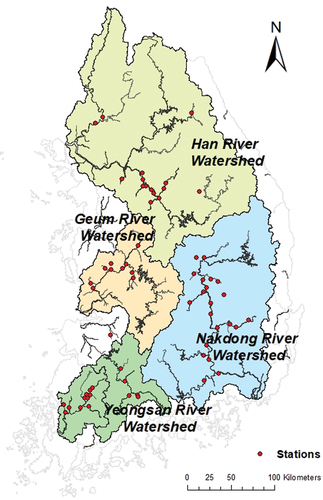
In this study, we considered 64 gauging stations in the Han, Nakdong, Geum, and Yeongsan rivers and tributaries and analysed the daily flow and sediment discharge data from 2007 to 2020. Most rivers in South Korea are alluvial sand-bed rivers, and the gauging stations used in this study are fully within the sand-bed transport zone. In these zones, streams merge and flow down mild slopes, thus transporting water and sediments along the riverbed. The sediment measurements were performed during both dry and flooding seasons, and most of the sediment transport occurred in flood events that predominantly comprised suspended loads. In addition, all measurement points were located downstream of hydraulic structures, such as dams or weirs, that were not affected by artificial hydraulic influences.

We included all the available data (officially recognized in South Korea) collected by the Korean Institute of Hydrological Survey (2008, 2009, 2010, 2011, 2012, 2013, 2014, 2015, 2016, 2017, 2018, 2019, 2020, 2021) to apply the MT approach for sediment discharge estimation. The Korean Institute of Hydrological Survey has been producing sediment discharge data and primary hydrological data related to flood and drought disasters in river watersheds in South Korea since 2007. Streamflow and sediment discharge data, including corresponding water level, flow velocity, water surface slope, and bed material grain size, observed from 2007 to 2020, were used in this study. Water surface slope data were not included in all datasets, and in the cases in which there were no water surface slope data, the energy slope (estimated based on the average velocity equation (Manning’s equation)) was estimated and used as the slope value.

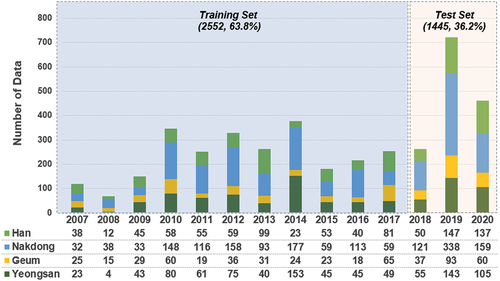
In total, 3997 data points were collected. Specifically, 721 data points were measured in 2019, whereas fewer than 69 data points were collected in 2008 (Fig. 2). Additionally, 1644 data points from the Nakdong River watershed, 921 from the Yeongsan River watershed, 897 from the Han River watershed, and 535 from the Geum River watershed were usable. Regarding the useable data, 63.8% of the data from 2007 to 2017 were used for MT training, and the remaining 36.89% were used for testing.

Figure 2. Distribution of useable sediment discharge data by watershed and year observed in the field from 2007 to 2020 in South Korea and the ratio of training and test datasets for model tree (MT).

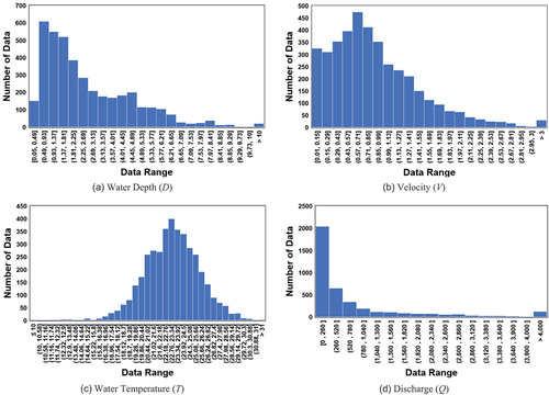
The measurement conditions and data range can be confirmed by the data presented in Fig. 3 and Table 1. Note that the model’s range of utilization estimated by data mining is related to the range of the collected and used datasets. Even though the collection of high-quality data is crucial, the derived model can be used in various conditions only when a broad range of data is comprehensively used for training. For the collection range of the data in this study, the distribution in terms of water depth ranged from 0.05 m to 13.92 m, with an average value of 2.65 m and a standard deviation of 2.0. The flow velocity ranged from 0.07 to 7.96 m/s, but in most of the data it was ≤3 m/s. The water temperature, which can indirectly confirm the data measurement season, was 23.13°C on average, and these measurements were concentrated in the summer season. This is because several streamflow and sediment discharge measurements were performed during this period as the rainfall occurrence in South Korea was mainly prevalent in the summer. The range of streamflow from the dry season to the flood season is distributed extensively, up to approximately 10 000 m³/s. Data ranges for each parameter are relatively wide because all datasets used in this study were collected from large rivers and small tributaries nationwide. Additionally, the ratio between maximum and minimum discharges (the high coefficient of flow regime) owing to the substantial increase in flow resulting from the concentration of floods for a certain period affects the broad distribution range of the observed datasets. Therefore, collecting a broad range of data, covering temporal and spatial changes, followed by their utilization in training, can contribute to expanding the scope of application of sediment discharge estimation models to be derived by MT.

Table 1. Coverage of long-term collected sediment datasets.

Dataset	Coverage	Elevation (m)	Width (m)	Area (m^2)	Velocity (m/s)	Depth (m)	Discharge (m^3/s)	Temperature (°C)	Slope (m/m)	Median bed material (mm)	Sediment discharge (tons/day)
Total	Minimum	−3.69	9.46	4.56	0.01	0.05	0.15	7.30	5.648E-09	0.26	0.02
	Maximum	31.23	637.27	4247.24	7.96	13.92	11317.34	32.44	0.2922	177.23	1 641 478.00
	Mean	2.66	212.33	707.86	0.88	2.65	717.94	23.13	0.0006	6.59	30 373.65
	Standard deviation (StdDev)	3.01	115.05	789.07	0.62	2.00	1197.03	2.62	0.0048	19.60	110 285.89
Han	Minimum	−0.40	16.58	4.56	0.02	0.08	0.15	7.30	4.37E-07	0.47	0.13
	Maximum	31.23	609.36	3455.70	7.96	9.02	10691.90	30.60	0.2922	151.00	1 641 478.00
	Mean	3.31	213.95	635.47	1.14	2.23	959.26	22.08	0.0012	5.59	58 416.95
	StdDev	5.48	129.15	714.01	0.80	1.72	1619.78	2.67	0.0101	17.48	175 527.85
Nakdong	Minimum	−3.69	9.46	4.78	0.01	0.05	0.78	9.30	5.648E-09	0.26	0.16
	Maximum	9.43	566.43	4247.24	3.81	13.92	11317.34	31.20	0.0221	86.88	1 485 669.80
	Mean	2.32	234.32	935.35	0.79	3.14	779.11	23.15	0.0005	4.19	22 540.21
	StdDev	1.69	113.00	976.78	0.51	2.44	1227.44	2.66	0.001	11.03	92 160.63
Geum	Minimum	0.09	39.58	14.90	0.01	0.33	0.21	13.10	3.805E-08	0.36	0.02
	Maximum	8.38	637.27	3822.92	2.27	6.25	4703.86	30.90	0.0018	50.58	624 768.29
	Mean	2.47	210.39	544.77	0.69	2.21	474.69	23.64	0.0003	3.25	21 623.47
	StdDev	1.47	98.48	520.66	0.49	1.47	702.50	2.59	0.0004	6.35	62 254.41
Yeongsan	Minimum	−1.45	18.49	8.56	0.01	0.25	1.28	11.80	9.902E-09	0.45	0.46
	Maximum	10.50	625.50	2368.70	2.95	6.97	6024.00	32.44	0.0092	177.23	712 949.90
	Mean	2.75	172.64	467.04	0.90	2.43	515.01	23.80	0.0004	13.78	22 126.82
	StdDev	1.79	101.86	418.97	0.57	1.35	743.15	2.18	0.0005	32.55	66 455.58

Figure 3. Distributions of data on water depth, velocity, water temperature and flow discharge.

2.2 Characterization of sediment discharge data

The new sediment discharge estimation model employing an MT creates sub-trees by correlating them with each other regardless of physical significance with the constructed data. Then, a multiple regression equation is provided for the collected data based on the use of the finally determined sub-tree. Before we applied the MT technique to develop a multiple regression equation based on the sub-trees, in accordance with the correlation values, a preliminary analysis was performed by Jang and Ji (2021) regarding the sediment discharge patterns by classifying station locations in different watersheds and main channels or tributaries. This information could be used to distinguish whether regional characteristics of the sediment discharge were reflected in the MT modelling process and to provide a better understanding of the MT’s final models.

In this study, a sediment transport curve method was adopted for total loads to define the power function, with the water discharge as the independent variable and the sediment discharge as the dependent variable. Table 2 summarizes sediment discharge rating curves. The relations are obtained by fitting river flow and sediment discharge data based on different river basins, the locations of stations, such as the main channel or tributary, and the total sizes of the datasets. The exponents (b) of the sediment discharge rating curves datasets measured at the stations in main streams are greater than those of tributaries. The high values of the exponent (b) for the main stream represent the steep slope of the curve, which indicates that the differences in sediment discharges between the low- and the high-flow rates are larger than those of the tributaries. This supports the fact that most sediment transport occurs during the flood season in the main channels of the Korean rivers. Additionally, the differences in the exponents (b) between main streams and tributaries in the cases of the Nakdong and Han rivers are greater than those between the Geum and Yeongsan rivers. However, this cannot be demonstrated by single factors because hydraulic, hydrological, geological, geographical, biological, and other factors affect the sediment load in the river in a complicated manner (Garcia 2008). Nevertheless, the Q–Qs relationship is extensively used to estimate sediment discharges for periods during which flow discharge data are available, but sediment data are not (e.g. Colby 1956, Higgins et al. 2016).

Table 2. Sediment rating curves based on field datasets.

Location of stations	Rivers	Qs = aQ^b
		a	b	R^2
Main channels and tributaries	Total	0.6725	1.4614	0.7785
	Han	1.6885	1.3788	0.7669
	Nakdong	0.5218	1.4318	0.7516
	Guem	0.3711	1.6385	0.8869
	Yeongsan	0.3563	1.6015	0.8646
Main channels	Total	0.0582	1.7344	0.7797
	Han	0.0034	2.0911	0.9274
	Nakdong	0.0033	2.0564	0.8614
	Guem	0.0284	1.9236	0.9011
	Yeongsan	0.1989	1.7034	0.8756
Tributaries	Total	0.6166	1.5379	0.8145
	Han	1.8529	1.404	0.8049
	Nakdong	0.4191	1.5634	0.7817
	Guem	0.2143	1.8443	0.9279
	Yeongsan	0.459	1.5508	0.8493

For Q_s = aQ^b, the unit for Q_s is tons/day and for Q is m³/s.

In this study, the collected sediment discharge dataset was compared directly with the estimated results by using six sediment transport equations that are extensively and practically used for river engineering in Korea (Fig. 4). Engelund and Hansen (1967), Ackers and White (1973), Brownlie (1981), and Van Rijn (1984) proposed semi-empirical equations based on energy concepts and showed that flow energy consumption is caused by the energy required for sediment transport. Yang’s (1973) approach is theoretical and is based on energy concepts and a unit stream power for sand; its coefficients are estimated computationally. By contrast, Shen and Hung (1972) proposed a regression equation based on empirical analysis.

Figure 4. Comparison of the measured total load and the bed-material load calculated by sediment transport equations.

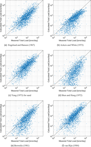
Figure 4 shows the comparison of measured and calculated total sediment load outcomes. Note that the wash load is not included in the total load estimated by the sediment transport equations, which means bed-material load. The overall occurrence pattern was relatively similar. However, a discrepancy of the log graph was observed in the sediment discharge estimation results, and the overall correlation was low. Specifically, the sediment discharge was underestimated by Shen and Hung’s (1972) equation, which was developed based on laboratory data with a sand bed. The equation proposed by Ackers and White (1973) was the best (among the six proposed equations) in reproducing the sediment occurrence pattern in the dataset based on correlation values. However, irrespective of the degree of agreement, caution is still recommended in terms of the scope of the equation’s application because it was developed based on limited ranges and scales of laboratory and field data. Despite the fact that all sediment transport equations are extensively used, the sediment discharge estimation may differ at each point.

2.3 Model tree

The MT approach, a representative method of prediction and classification in data mining, is known to be a highly explicit and straightforward approach for interpreting results from diverse and large quantities of data (Witten et al. 2016). In this method, only the critical variables are selected to estimate the dependent value among those variables that have influences. Subsequently, this method provides a linear relationship between the explanatory variables and the response variable. Given that several sub-trees (which are more relevant compared with the initial tree) are provided to generate a linear relationship, the latter is affected to a lesser extent by outliers compared with a non-linear relationship case (Witten et al. 2016).

The MT approach is based on a process associated with the separation of data into sub-trees. Notably, sub-trees resulting from partitioning become more homogeneous in terms of dependent variables. As a result, they will certainly produce better predictions or classification rules than those provided by the initial tree. The MT approach entails tree growth, pruning, and smoothing processes. First, the growth of a tree is divided into several branches. Branches are divided when the standard deviation reduction (SDR), expressed by Equation (1)(1) $\mathrm{S}\mathrm{D}\mathrm{R}=\mathrm{S}\mathrm{D}\left(T\right)-\sum _i\frac{\left|T_i\right|}{\left|T\right|}\times sd\left(T_i\right),$(1) , is the maximum (Quinlan 1992, Wang and Witten 1996).

(1) $\mathrm{S}\mathrm{D}\mathrm{R}=\mathrm{S}\mathrm{D}\left(T\right)-\sum _i\frac{\left|T_i\right|}{\left|T\right|}\times sd\left(T_i\right),$(1)

where T is the entire sample set of the dependent variable, T_i is the sub-tree set of the dependent variable segmented into subsample sets, SD is the standard deviation, and $\left|T\right|$ and $\left|T_i\right|$ are the sizes of the entire and subsample sets, respectively, and are expressed by the numbers of elements. The grouping of each independent variable is assessed based on the SDR of each sub-tree set. After the SD is calculated based on the entire sample set T, including unnecessary branches, the SDR for the sub-tree set Ti is determined by dividing this set into random temporary sub-trees for each independent variable. Among the randomly divided sub-trees, the one with the largest SDR is selected and pruned, after which a lower tree is established. The pruning and termination conditions are selected by referring to the MT classification rule. A sub-tree that satisfies the SDR criterion on the entire dataset was pruned. By repeating this process, growth and pruning are conducted continuously, and when the SDR reaches the desired value, or when the number of remaining elements after grouping is too small to perform multiple regression analysis, the tree growth is terminated. When the final sub-tree is constructed, multiple linear regression is performed. Bhattacharya et al. (2007) can be referenced to understand the classification process and concept of MT.

When selecting the growth and termination conditions of the tree, the influence of the minimum number of data points is minimized so that the tree can grow sufficiently. Witten et al. (2016) explained that the structure of an MT could be established for multiple regression analysis regardless of the fact that the minimum number of data points was four. Therefore, in this study, the minimum number of data points under the MT classification conditions was set to four. Furthermore, the SDR was set at 5% because extremely small SDR values would lead to the formation of unnecessarily numerous trees, thus making the new equation less usable. In other words, if the SDR does not decrease by more than 5%, even after classification, the growth of the tree ends.

2.4 Parameter determination and model performance evaluation method

Kennedy and Brooks (1963) used the relationship between independent and dependent variables related to the fluvial characteristics to select the dimensional variables related to sediment discharge. As shown in Equation (2)(2) $Q_s=f\left(\upsilon ,\rho ,{\rho }_s,d_s,{\sigma }_g,\omega ,g,Q,W,DR,V,S,f\right),$(2) , independent variables in alluvial streams include fluid properties, sediment properties, gravitational acceleration, and other flow-related variables.

(2) $Q_s=f\left(\upsilon ,\rho ,{\rho }_s,d_s,{\sigma }_g,\omega ,g,Q,W,DR,V,S,f\right),$(2)

where $Q_s$ represents the sediment discharge, $\upsilon$ is the kinematic viscosity of the fluid, $\rho$ is the density of the fluid, ${\rho }_s$ is the density of the sediment particles, $d_s$ is the geometric mean size of the bed material, ${\sigma }_g$ is the geometric standard deviation of the size of the bed material, $\omega$ is the geometric mean settling velocity of the sediment particles, $g$ is the acceleration due to gravity, $Q$ represents flow discharge, $W$ is the channel’s width, $h$ is the section-averaged depth, $R$ is the hydraulic radius, $V$ is the reach-averaged flow velocity, $S$ is the bed slope, and $f$ is the Darcy friction factor. Independent variables with constant values are not affected by sub-tree processes. For example, fluid properties and gravitational acceleration have constant values regardless of their group. Therefore, the use of an MT to develop the sediment discharge model does not entail constant values. By contrast, only variables such as reach-averaged flow velocity ($V$), cross-sectional mean depth ($D$), water surface or energy slope (S), geometric mean size of bed materials ($d_{50}$), and channel width ($W$) are valid. The various combinations of parameters are already examined based on the sensitivity analysis performed by Jang (2017). Based on the results from Jang (2017), the dimension parameters of $V$, $D$, S, $d_{50}$, and $W$ were selected for the development of the MT models in this study.

The performances obtained using the training and test sets were evaluated by using various measures of prediction accuracy. In this study, the mean discrepancy ratio ($\bar{R}$), root mean square error (RMSE), mean absolute percentage error (MAPE), and correlation coefficient ($r$) between the measured and predicted sediment discharges were evaluated. The equations for various measures of prediction accuracy are defined in the Appendix.

3 Results

3.1 Training of sediment discharge estimation models

The five variables – reach-averaged flow velocity ($V$), cross-sectional mean depth ($D$), water surface or energy slope (S), geometric mean size of bed materials ($d_{50}$), and channel width ($W$) – described in Section 2.4 were adopted for the training of the sediment discharge model using the MT approach. As mentioned earlier, 63.8% of the data from 2007 to 2017 were used for MT training. MT training cases were categorized based on the combination of five variables: one case in which all five variables were considered (Case 1) and cases in which one of the variables was excluded (Cases 2 to 6) (Table 3). Cases 2–6 were established to examine the extent of the variation of the estimated sediment discharge when any one of the five variables was excluded. Combinations of cases in which two or more variables were excluded were not considered in this training paradigm. The sub-tree creation conditions were set to be the same as those for the raw data with an SDR of 5% and at least four factors within the group. As shown in Fig. 5, the modelling resulted in the largest group of 38 in Case 3 and the smallest group of 10 in Case 6. This does not mean that the generation of many sub-trees results in better accurate model estimation; however, as the number of sub-trees increases, the range within which the relationships can be estimated correctly becomes more comprehensive. If the sub-tree is relatively small, it can be interpreted as sufficient to provide a regression model despite the small sub-group.

Table 3. Mean discrepancy ratio ($\bar{R}$), root mean square error (RMSE), mean absolute percentage error (MAPE), and correlation coefficient ($r$) $\bar{R}$ values based on the measured data used for training.

Note	$\bar{R}$	RMSE	MAPE	$r$
Case 1: $D$, $S$, $W$, $V$, $d_{50}$	1.730	99 676	118.78	0.71
Case 2: $D$, $S$, $W$, $d_{50}$	2.443	93 691	192.46	0.75
Case 3: $S$, $W$, $V$, $d_{50}$	1.722	83 924	117.01	0.80
Case 4: $D$, $S$, $V$, $d_{50}$	1.834	92 057	130.23	0.75
Case 5: $D,V,W,d_{50}$	1.738	100 113	119.72	0.71
Case 6: $D$, $S$, $W$, $V$	1.871	98 422	134.45	0.71

Figure 5. Sub-tree distribution created for each studied case.

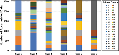
We compared the measured sediment discharge data with the results calculated by the sediment discharge model developed by MT for each tested case. The bar on the right indicates the sub-tree groups. Owing to the characteristics of the log graph, the differences in the values for each exact point were analysed separately according to the goodness of fit. The pattern of occurrence, degree of agreement, and scatter plot can be viewed in Fig. 6. All cases (Cases 1–6) exhibit characteristics of the measured sediment discharge and similar occurrence patterns. Therefore, the degree of dispersion based on the streamflow range required arithmetic identification (Table 3).

Figure 6. Comparison of sediment discharges that were measured and those calculated by model tree based on training data.

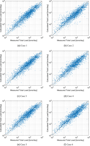
For $\bar{R}$, which can distinguish a simple degree of discrepancy, all cases yielded overestimated outcomes with values >1 (compared with the optimal value of 1); the average value was 1.89. The RMSE consisted of 94,000 margins of error on average. Case 5 yielded a considerable difference, which was approximately equal to 100,000. The quantitative difference in the RMSE can be confirmed through the MAPE. When 100% was set as the optimal value, the simple average value differed by 37.5%, regardless of whether outcomes were underestimated or overestimated. The Pearson correlation coefficient yielded optimal average values ≥0.74. Considering the degree of inconsistency and MAPE for each case, Case 1 used five variables and was judged to be the most appropriate. A cautious approach should be adopted when using Case 2, which did not consider the flow velocity, and Case 5, which did not consider the slope.

Nevertheless, field application of the MT method is expected based on considerations of the limitation of sediment discharge estimation. In the existing sediment transport equation, differences of up to several tens of thousands of times occur. Although the method of estimating sediment discharge was presented in this study based on statistical rules and patterns and in accordance with relationships within large-scale data, it is not associated with any physical model mechanism with the exception of the selection of independent parameters that affect sediment transport. However, the method makes it possible to estimate the statistical sediment discharge even if any one variable is excluded, thus contributing to rational and prompt application.

3.2 Testing of sediment discharge estimation models

The sediment discharge estimation model developed in the training process using the MT method was tested by applying data from 2018 to 2020 for the validation of the method application for sediment discharge estimation (Fig. 7). Compared with the training set, the measured sediment discharge generation pattern yielded a relatively good performance for the agreement with estimated data, and the method was implemented effectively, as shown in Fig. 4.

Figure 7. Comparison of sediment discharges that were measured and those calculated by model tree based on test data.

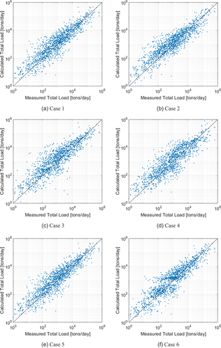
Similar to the training, the testing results were compared with the measured data, as shown in Table 4. The results of Case 1, which applied all the variables in the training process, were optimal. Although it was not expected that utterly consistent results would be obtained in testing, it was interesting that Case 6, which excluded the median particle size, yielded the highest $\bar{R}$ value of 2.43. In comparison, the average $\bar{R}$ value for training was 1.89, and the overall $\bar{R}$ value associated with testing was 2.96. Notably, the average RMSE of all cases was 31 574, which was considerably lower than that of the testing process. Conversely, considering that the average $\bar{R}$ increases and the MAPE exceeds 200%, it can be estimated that the sediment discharge from 2018 to 2020 is much smaller than that from 2007 to 2017. This is because an average sediment discharge error of approximately 30 000 tons per day per point is equivalent to more than 200% of the measurements.

Table 4. $\bar{R}$, RMSE, MAPE, and r values based on the measured data used for testing.

Note	$\bar{R}$	RMSE	MAPE	$r$
Case 1: $D$, $S$, $W$, $V$, $d_{50}$	2.637	31 853	194.95	0.70
Case 2: $D$, $S$, $W$, $d_{50}$	2.814	26 674	214.45	0.79
Case 3: $S$, $W$, $V$, $d_{50}$	4.066	31 340	336.34	0.69
Case 4: $D$, $S$, $V$, $d_{50}$	3.099	38 062	248.11	0.61
Case 5: $D,V,W,d_{50}$	2.688	31 704	199.10	0.70
Case 6: $D$, $S$, $W$, $V$	2.430	29 811	178.60	0.73

As a result, based on the training and testing process of the MT, it was determined that the feasibility of the MT method for the estimation of sediment discharge would be higher compared with the outcomes in Fig. 4, based on the existing sediment transport equations. Local and temporal characteristics can be considered because various conditions are generated by numerous sub-trees owing to MT modelling. For example, two cases with the same streamflow conditions and different sediment discharge patterns before and after flooding can be distinguished into different sub-trees. In addition, different sediment discharges can be estimated according to bed sediment materials, even for the same flow velocity conditions.

3.3 Sediment discharge estimation using the MT

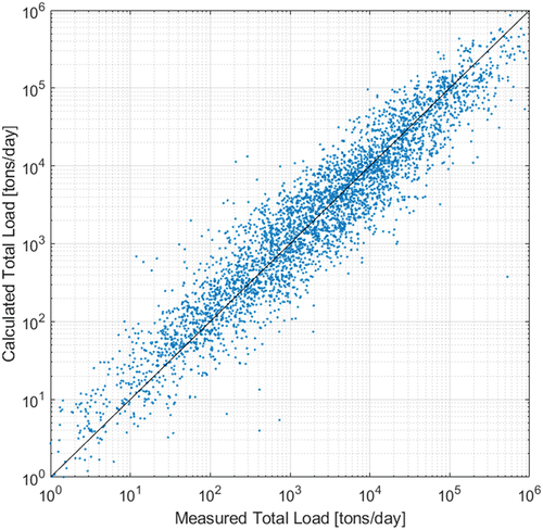
The MT method used for modelling sediment discharge was examined based on the training data from 2007 to 2017 and the test data from 2018 to 2020. With respect to the final process of the MT approach, sediment discharge estimation models with higher estimation accuracy were derived by using all measured data from 2007 to 2020. The previous sections focused on testing the construction and applicability of the proposed method, and this section is intended to enable users to actually use the model for estimating sediment discharge. Fifty-three sub-models were constructed to estimate sediment discharge as a result of the model creation based on the applicable ranges of parameters (Fig. 8). A wider range of data could be secured because more data were utilized. Furthermore, more sub-trees were formed to derive high-accuracy models within such a broad range of data, as a more detailed sub-tree condition is expected to be able to cover a vast amount of data according to the process condition. The results showed higher sophistication than the test model. A graph comparing with the measured sediment discharge (Fig. 8) shows that the results are close to the optimal fit. For example, while the fit was 1.556, the MAPE yielded an optimum value of 99.18% and an error range of only 1%. The average RMSE was 69 038, and the Pearson correlation coefficient was 0.82; this was the highest correlation coefficient achieved compared with training and testing data.

Figure 8. Comparison of sediment discharges that were measured and those calculated based on the final model tree models.

Compared with other data-based methods and ML, the strongest advantage of the MT method is that it produces a model in the form of an equation for estimating sediment discharge in addition to the estimation results. Equation (3)(3) $Q_s=a\ast W^b\ast V^c\ast D^d\ast S^e\ast {d_{50}}^f$(3) expresses the form of sediment discharge estimation models derived from the MT application. The independent parameters of flow system variables D, S, W, V, and d₅₀ were selected for MT modelling. The applicable parameter ranges, coefficients, and exponents were determined by the MT modelling results (Table 5). Because the final derived model has coefficients determined by a simple conditional method, it is much easier and simpler to access than the existing sediment transport equation. In addition, the dataset acquired in the target section of the study is expected to be applicable to more conditions because it covers a broader range.

(3) $Q_s=a\ast W^b\ast V^c\ast D^d\ast S^e\ast {d_{50}}^f$(3)

Table 5. Application conditions and determination coefficients of the sediment-transport equation of the MT.

Parameter ranges and conditions					Coefficient and exponents of sediment discharge model by MT
V (m/s)	D (m)	W (m)	d50 (mm)	S (m/m)	a	b	c	d	e	f
V ≤ 0.25	D ≤ 0.66				9.794294	0.8821	1.1143	0.788	0.153	−0.2349
V ≤ 0.10	0.66 < D				25.80582	0.5073	1.1863	0.8627	0.0023	−0.1289
0.10 < V ≤ 0.25	0.66 < D ≤ 0.77	W ≤ 66.55	d50 ≤ 1.23		0.000793	2.9423	1.8128	−1.1159	−0.0853	0.2879
0.10 < V ≤ 0.25	0.66 < D ≤ 0.77	66.55 < W ≤ 118.63	d50 ≤ 1.23		0.000806	2.9423	1.8128	−1.1159	−0.0853	0.2879
0.10 < V ≤ 0.25	0.77 < D ≤ 3.64	W ≤ 118.63	d50 ≤ 1.23		0.004014	2.732	1.8128	−0.8739	−0.0016	0.2879
0.10 < V ≤ 0.25	0.66 < D ≤ 3.64	W ≤ 118.63	1.23 < d50 ≤ 2.67		0.383429	1.5671	1.8544	−0.2598	−0.0853	0.3215
0.10 < V ≤ 0.25	0.66 < D ≤ 1.55	W ≤ 118.63	2.67 < d50		1.967965	1.1863	2.159	0.4012	−0.0853	−0.0138
0.10 < V ≤ 0.25	1.55 < D ≤ 3.64	W ≤ 118.63	2.67 < d50		1.232938	1.2495	1.9891	0.4594	−0.0853	−0.0138
0.10 < V ≤ 0.13	0.66 < D ≤ 3.64	118.63 < W ≤ 131.63			791.0807	0.0622	2.0187	0.422	−0.0811	−0.0138
0.13 < V ≤ 0.25	0.66 < D ≤ 3.64	118.63 < W ≤ 131.63			640.2124	0.0622	1.7665	0.422	−0.0811	−0.0138
0.10 < V ≤ 0.25	0.66 < D ≤ 3.64	131.63 < W ≤ 248.39			311.8119	0.178	2.0297	0.745	−0.0811	−0.0138
0.10 < V ≤ 0.25	0.66 < D ≤ 3.64	248.39 < W			2684.366	0.3393	1.3591	1.0938	0.2784	1.515
0.10 < V ≤ 0.25	3.64 < D				3929.628	−0.2638	1.8306	1.2737	−0.0132	−0.0138
0.25 < V ≤ 0.72	D ≤ 0.70	W ≤ 71.74			0.318351	0.26	2.3221	0.6744	−0.7418	−0.096
0.25 < V ≤ 0.48	D ≤ 0.70	71.74 < W		S ≤ 0.00043	1638.932	0.1655	−0.0808	2.1407	0.3237	−0.2183
0.25 < V ≤ 0.48	D ≤ 0.70	71.74 < W		0.00043 < S	20074.39	0.1655	−0.3896	2.8892	0.5122	−0.6408
0.48 < V ≤ 0.72	D ≤ 0.70	71.74 < W			1523.248	0.1655	0.1648	2.158	0.1862	−0.0995
0.25 < V ≤ 0.54	0.70 < D ≤ 1.51	W ≤ 97.03	d50 ≤ 0.73		1.998107	0.9507	1.8527	−0.2394	−0.0697	−2.4461
0.25 < V ≤ 0.54	0.70 < D ≤ 1.51	97.03 < W ≤ 196.96	d50 ≤ 0.73		7.658376	0.6613	1.8527	−0.2394	−0.0697	−2.4461
0.25 < V ≤ 0.54	0.70 < D ≤ 1.51	W ≤ 196.96	0.73 < d50 ≤ 2.04		77.78122	0.2963	2.7812	−0.1081	−0.0697	−1.7275
0.25 < V ≤ 0.54	0.70 < D ≤ 1.51	W ≤ 196.96	0.82 < d50 ≤ 2.04		54.17394	0.2963	0.3482	0.9818	−0.0697	−0.4231
0.25 < V ≤ 0.54	0.70 < D ≤ 1.51	196.96 < W	d50 ≤ 2.04		27.85187	0.3896	0.4854	2.6104	−0.1368	1.4777
0.25 < V ≤ 0.54	0.70 < D ≤ 1.51		2.04 < d50		32.41755	0.5893	1.0743	1.297	0.006	−0.3028
0.54 < V ≤ 0.72	0.70 < D ≤ 1.02	W ≤ 74.07			0.114075	0.7572	2.9037	−1.3878	−0.644	0.0197
0.54 < V ≤ 0.72	0.70 < D ≤ 1.02	74.07 < W ≤ 107.13			8587.818	−1.4717	4.6341	−1.3284	−0.6237	0.0197
0.54 < V ≤ 0.72	1.02 < D ≤ 1.51	W ≤ 107.13		S ≤ 0.00029	27.33314	0.6525	0.5846	−0.2237	0.006	0.0846
0.54 < V ≤ 0.72	1.02 < D ≤ 1.51	W ≤ 107.13		0.00029 < S	0.005212	2.5413	−1.5303	−0.5752	0.006	0.1307
0.54 < V ≤ 0.72	0.70 < D ≤ 1.51	107.13 < W			2602.167	0.2122	4.6441	0.2596	0.006	−0.2373
0.25 < V ≤ 0.72	1.51 < D				197.4726	1.1047	1.6924	0.9573	0.3539	−0.1033
0.72 < V ≤ 1.25	D ≤ 1.81	W ≤ 70.04			0.164244	0.5692	2.329	0.1741	−0.7533	−0.0236
0.72 < V ≤ 1.25	D ≤ 1.81	70.04 < W ≤ 99.88			7.56E+12	−5.0728	4.6177	0.1741	−0.0574	−0.0236
0.72 < V ≤ 1.25	D ≤ 1.81	99.88 < W ≤ 216.59			7656.422	0.5572	1.2224	2.0111	0.5611	−0.2671
0.72 < V ≤ 1.25	1.81 < D	W ≤ 109.84			14.50074	0.6721	0.9002	1.6872	−0.0398	0.071
0.72 < V ≤ 1.25	1.81 < D	109.84 < W ≤ 129.28			125.2736	0.5621	1.7355	0.3001	−0.0398	0.3251
0.72 < V ≤ 0.87	1.81 < D	129.28 < W ≤ 216.59	d50 ≤ 0.48		0.001381	2.1933	1.3243	0.3226	−0.3464	0.0863
0.87 < V ≤ 1.04	1.81 < D	129.28 < W ≤ 184.93	d50 ≤ 0.48		0.657113	1.4187	1.1886	−0.0543	−0.1818	0.0863
0.87 < V ≤ 1.04	1.81 < D	184.93 < W ≤ 216.59	d50 ≤ 0.48		0.407669	1.6524	1.1886	−0.5254	−0.1818	0.0863
0.72 < V ≤ 1.04	1.81 < D	129.28 < W ≤ 216.59	0.48 < d50	S ≤ 0.00018	0.000819	1.8646	0.4651	0.4526	−0.6621	0.1648
0.72 < V ≤ 1.04	1.81 < D	129.28 < W ≤ 216.59	0.48 < d50	0.00018 < S	364.8915	0.2972	0.4651	0.3751	−0.0735	0.0642
1.04 < V ≤ 1.25	1.81 < D	129.28 < W ≤ 216.59			1374.988	0.1742	2.8009	0.1748	−0.0452	0.0442
1.25 < V	D ≤ 1.78	W ≤ 121.03	d50 ≤ 1.18		0.502379	1.3393	1.0981	0.1011	−0.4246	−0.0588
1.25 < V	D ≤ 1.15	W ≤ 121.03	1.18 < d50		9.158661	1.0289	0.4669	0.9627	−0.1789	0.3426
1.25 < V	1.15 < D ≤ 1.78	W ≤ 121.03	1.18 < d50		3.781422	0.9906	1.8028	0.1011	−0.1789	0.3125
1.25 < V	D ≤ 1.78	121.03 < W ≤ 216.59			234.9799	0.9539	0.4301	1.2363	0.2335	−0.2687
1.25 < V	1.78 < D	W ≤ 216.59			16.32341	1.5886	1.4638	1.3535	0.3552	−0.2426
0.72 < V ≤ 1.36		216.59 < W			26.18011	1.2335	2.549	0.9729	0.2211	−0.1842
1.36 < V ≤ 2.03	D ≤ 4.15	216.59 < W			12.64422	1.55	1.6143	0.1002	0.1861	−0.2411
1.36 < V ≤ 1.49	4.15 < D	216.59 < W			10 905.25	0.2086	1.0422	0.1017	0.0047	−0.0677
1.49 < V ≤ 2.03	4.15 < D	216.59 < W	d50 ≤ 0.80		10 750.42	0.3043	2.3109	−0.2304	0.0047	−0.0657
1.49 < V ≤ 2.03	4.15 < D	216.59 < W	0.80 < d50		421.0704	0.8579	0.6765	0.1017	0.0047	−0.0639
2.03 < V	D ≤ 4. 74	216.59 < W ≤ 370.55			332368.6	−0.3082	0.2382	0.5194	0.0607	0.0483
2.03 < V	D ≤ 4.74	370.55 < W			1334.884	0.8604	0.0085	0.2224	0.1152	0.2958
2.03 < V	4.74 < D	216.59 < W			16.70152	0.3858	2.9989	0.2264	−0.6064	−0.1496

where $W$ is channel width (m), $V$ is flow velocity (m/s), $D$ is mean depth (m), $S$ is water surface or energy slope (m/m), $d_{50}\left(mm\right)$ is the geometric mean size of bed materials and $a,b,c,d,e\mathrm{a}\mathrm{n}\mathrm{d}f$ are constants.

4 Discussion

Approximately 4000 data points collected from the measurement field from small streams to large rivers in South Korea contributed to a better understanding of data-based sediment transport characteristics and to deriving the sediment discharge equation using the MT data-mining technique. Section 2.2 on the characterization of sediment discharge data could be explained further in relation to the scope of data used in the development of the sediment transport equation, which is related to the regional characteristics of the target section to be estimated. South Korean rivers are characterized by steep bed slopes owing to mountain river sections upstream, lateral channel migration limits owing to levee construction downstream, a wide range of maximum and minimum streamflow ratios throughout the year, and concentrated floods in summer. As previous studies have identified inaccuracies in sediment transport equations (e.g. Bayram et al. 2001, Yang et al. 1996), there are limitations in attempting to describe this process in accurate mathematical terms. Moreover, it is challenging to find the best equation among the existing sediment transport equations compared with sediment discharge data observed in rivers with such characteristics described above.

As Jang and Ji (2021) pointed out, large deviations were produced when the existing sediment transport equations were applied to the rivers in South Korea. The first investigation, by Bhattacharya et al. (2007), of using MT in sediment transport modelling was comparable in accuracy with others developed during the last several decades. However, in this study, the MT application with approximately 4000 sediment discharge data points collected in the field produced a state-of-the-art regression equation set which provides a better fit to the measured data and higher accuracy with wider applicable ranges of input parameters.

The results derived through the sensitivity analysis and those based on training and testing steps of the sediment discharge MT-based estimation indicated that the agreement between the measured values and predicted values obtained using the MT is somewhat inferior when a specific input variable is missing for modelling the equation. Therefore, the smartest way to secure accuracy of the sediment discharge prediction derived by MT models is to include all five physical variables with a dominant influence on sediment transport in the application of the MT on this dataset. According to the results of the MT in the training, testing, and final model construction processes, the higher the number of data points and variables applied, the higher the accuracy and consistency produced.

The equation derived by the MT can be actively applied to numerical modelling that predicts river morphological changes, such as bed elevation changes, after the estimation of the sediment transport amount for each cross-section by applying all the given independent variable conditions. In addition, the same observation data applied to the MT can be used to derive a regression equation as a relational expression between flow rates and sediment discharge, followed by the derivation of data on the upstream sediment inflow of the river bed variation modelling. The sediment transport equation for bed change modelling is selected after the derivation of the flow and sediment discharge relationship based on measured data and comparison of these data with the results calculated by the sediment transport equations. Furthermore, after applying this equation to the hydraulic and bed material conditions of each cross-section, it is used to calculate the sediment transport capacity and riverbed variations.

The advantage of the MT application for sediment discharge estimation pertains to the fact that it is useful to derive a spatial and temporal model for the rivers from which sediment data are secured. For example, it is possible to derive a sediment discharge prediction model for the river by adjusting the dataset for different periods before and after artificial river facilities are installed. The procedures and methods used to develop sediment discharge estimation equations for specific points, watersheds, and periods following the application of the MT can be guided using the results described in this study. In particular, variable selection and modelling can be derived by referring to the flowchart presented in Jang (2017).

5 Conclusions

By using the MT data mining technique, sediment discharge models were developed with around 4000 field data points collected from rivers in Korea during the time period 2007–2020. Considering fluvial parameters related to sediment transport and flow systems for sediment discharge estimation, the performance of the MT procedure was analysed based on the training and testing processes, and the final model sets for sediment discharge estimation were presented as an equation-type index according to the applicable ranges of fluvial conditions. When the five variables of $D$, $S$, $W$, $V$, and $d_{50}$ were used, the MT models yielded the most optimal agreement overall, covering a wide range of applications.

The MT method has the practical advantages of being able to perform a sensitivity analysis based on variable selection for model development and data range, and being able to present the final model result in the form of an equation. There is a limit to the presentation of a governing equation that can quantify the amount of sediment transport based only on the physical and theoretical approaches. The results of this study support the conclusion that it is feasible to use the data mining MT method that analyses the complexity of sediment transport based on the interpretation and trends implied by the dataset. If long-term sediment data are valid, based on actively utilizing the advantage of the MT method – that presents a model of the relational form between sediment discharge and physical independent variables – it is concluded that developing and using the sediment discharge estimation equation from the MT constitutes the most effective method.

Disclosure statement

No potential conflict of interest was reported by the authors.

Data availability statement

The authors confirm that the data supporting the findings of this study are available within the article or its supplementary material.

Supplementary material

Supplemental data for this article can be accessed online at https://doi.org/10.1080/02626667.2023.2221790

Additional information

Funding

Research for this paper was carried out under the Korea Institute of Civil Engineering and Building Technology (KICT) Research Program (project no. 20230115-001, Development of IWRM-Korea Technical Convergence Platform Based on Digital New Deal) funded by the Ministry of Science and ICT of Korea.

Appendix

Mean discrepancy ratio

To determine the fit of the estimated values to the measured values, the mean discrepancy ratio ($\bar{R}$), which is the most commonly used estimation method, was used for the analysis here (Equation A1), and in previous studies by Nagy et al. (2002), Khullar et al. (2010), and Yang and Simões (2005). If R has a value less than 1, the estimated value is smaller than the observed value. The closer the value of R to 1, the better the fitness.

(A1) $\bar{R}=\frac{1}{n}{\sum }_{i=1}^n\left(\frac{y_i}{x_i}\right),$(A1)

where $n$ is the total number of data points, $x_i$ is a dependent variable of data point $i$, and $y_i$ is the predicted value for data point $i$.

RMSE

The RMSE is the arithmetic mean of the sum of the squares of the residuals of each data point – that is, the mutual deviation between the observed and the estimated values. This measure is used to generalize the standard deviation (SD) and is often used to determine the difference between actual and estimated values. It indicates the degree of error for individual observations (Ma and Huang 2016); the smaller the value, the higher the precision. In general, approximately 68% of the total data are within ±1 RMSE around the regression line, and approximately 95% of the data are within ±2 RMSE around the regression line. The RMSE is expressed by Equation (A2).

(A2) $\mathrm{R}\mathrm{M}\mathrm{S}\mathrm{E}=\sqrt{\frac{1}{n}\sum _{i=1}^n{\left(x_i-y_i\right)}^2}$(A2)

MAPE

The mean absolute percentage error (MAPE) was used to determine the percentage of all absolute errors and was not related to the sign of the estimated and measured values (Equation A3). Determining the MAPE is one way to compare the predicted and observed results, while ignoring the degree of underestimation or overestimation (Ma and Huang 2016). Unlike the RMSE, which represents the quantitative error, the MAPE shows the ratio of the error to the observed value. Further, in contrast with the RMSE, the MAPE can be employed to determine whether the data are underestimated or overestimated, with the optimal value being 100%.

(A3) $\mathrm{M}\mathrm{A}\mathrm{P}\mathrm{E}=\frac{1}{n}\sum _{i=1}^n\frac{\left|x_i-y_i\right|}{x_i}\times 100$(A3)

Pearson correlation coefficient

In the cases of the $\bar{R}$, RMSE, and MAPE, there is a limitation in determining the degree of density of data or the relationship between two variables. Therefore, to measure the direction and strength of the linear relationship between two variables, Equation (A4) was used to estimate the correlation coefficient ($r$). Note that $r$ always ranges from −1 to 1, and the closer its value to 1, the stronger the linear relationship. A perfect correlation exists at a value of 1 (Jain 2001).

(A4) $r=\frac{1}{n-1}{\sum }_{i=1}^n\left(\frac{x_i-\bar{x}}{{\sigma }_x}\right)\left(\frac{y_i-\bar{y}}{{\sigma }_y}\right),$(A4)

where $\bar{x}$ and $\bar{y}$ are the mean values for each group, and ${\sigma }_x$ and ${\sigma }_y$ are the SDs corresponding to each group.

References

- Ackers, P. and White, W.R., 1973. Sediment transport: new approach and analysis. Journal of Hydraulics Division, 99 (hy11), 1973. doi:10.1061/JYCEAJ.0003791
- Alemdag, S., et al., 2016. Modeling deformation modulus of a stratified sedimentary rock mass using neural network, fuzzy inference and genetic programming. Engineering Geology, 203, 70–82. doi:10.1016/j.enggeo.2015.12.002
- American Society of Civil Engineers, 1982. Relationships between morphology of small streams and sediment yield. Journal of Hydraulics Division, 108 (11), 1328–1365. doi:10.1061/JYCEAJ.0005936
- Azamathulla, H.M., et al., 2010. Machine learning approach to predict sediment load–a case study. Clean–Soil, Air, Water, 38 (10), 969–976. doi:10.1002/clen.201000068
- Bagnold, R.A., 1980. Empirical correlation of bedload transport rates in flumes and natural rivers. Proceedings of the Royal Society of London, Series A Mathematics Physical Sciences, 372 (1751), 453–473. doi:10.1098/rspa.1980.0122.
- Bagnold, R.A., et al., 1988. The Physics of Sediment Transport by Wind and Water. USA: American Society of Civil Engineers.
- Bayram, A., et al., 2001. Cross-shore distribution of longshore sediment transport: comparison between predictive formulas and field measurements. Coastal Engineering, 44 (2), 79–99. doi:10.1016/S0378-3839(01)00023-0
- Bhattacharya, B., Price, R.K., and Solomatine, D.P., 2007. Machine learning approach to modeling sediment transport. Journal of Hydraulics Engineering, 133 (4), 440–450. doi:10.1061/(ASCE)0733-9429(2007)133:4(440)
- Brownlie, W.R., 1981. Prediction of flow depth and sediment discharge in open channels. Pasadena, California: California Institute of Technology.
- Buyukyildiz, M. and Kumcu, S.Y., 2017. An estimation of the suspended sediment load using adaptive network based fuzzy inference system, support vector machine and artificial neural network models. Water Resources Management, 31 (4), 1343–1359. doi:10.1007/s11269-017-1581-1
- Colby, B.R., 1956. Relationship of sediment discharge to streamflow (No. 56–27). Washington, DC: US Department of Interior, Geological Survey, Water Resources Division.
- Engelund, F. and Hansen, E., 1967. A monograph on sediment transport in alluvial streams. Copenhagen, Denmark: Technical University of Denmark.
- Garcia, M., ed., 2008. Sedimentation engineering: processes, measurements, modeling, and practice. USA: American Society of Civil Engineers.
- Higgins, A., et al., 2016. Suspended sediment transport in the Magdalena River (Colombia, South America): hydrologic regime, rating parameters and effective discharge variability. International Journal of Sediment Research, 31 (1), 25–35. doi:10.1016/j.ijsrc.2015.04.003
- Jain, S.K., 2001. Development of integrated sediment rating curves using ANNS. Journal of Hydraulics Engineering, 127 (1), 30–37. doi:10.1061/(ASCE)0733-9429(2001)127:1(30)
- Jang, E.K., 2017. Sediment Discharge Assessment for Rivers using Model Tree in Data Mining. Thesis (PhD). Yongin, Korea: Myongji University.
- Jang, E.K. and Ji, U., 2021. Sediment load characteristics in South Korean rivers and assessment of sediment transport formulas. KSCE Journal of Civil Engineering, 25 (12), 4646–4660. doi:10.1007/s12205-021-1070-1
- Julien, P.Y., 2010. Erosion and sedimentation. Cambridge, UK: Cambridge University Press.
- Julien, P.Y., 2018. River mechanics. Cambridge, UK: Cambridge University Press.
- Kakaei Lafdani, E., Moghaddam Nia, A., and Ahmadi, A., 2013. Daily suspended sediment load prediction using artificial neural networks and support vector machines. Journal of Hydrology, 478, 50–62. doi:10.1016/j.jhydrol.2012.11.048
- Kang, W., et al., 2019. Sediment yield for ungauged watersheds in South Korea. KSCE Journal of Civil Engineering, 23 (12), 5109–5120. doi:10.1007/s12205-019-0085-3
- Kang, W., Lee, K., and Jang, E.K., 2022. Evaluation and validation of estimated sediment yield and transport model developed with model tree technique. Applied Sciences, 12 (3), 1119. doi:10.3390/app12031119
- Kargar, K., et al., 2019. Sediment transport modeling in open channels using neuro-fuzzy and gene expression programming techniques. Water Science Technology, 79 (12), 2318–2327. doi:10.2166/wst.2019.229
- Kennedy, J.F. and Brooks, N.H., 1963. Laboratory study of an alluvial stream at constant discharge. In: Federal inter-agency sedimentation conference, June 1965, Washington, DC, 320–330.
- Khosravi, K., et al., 2018. Quantifying hourly suspended sediment load using data mining models: case study of a glacierized Andean catchment in Chile. Journal of Hydrology, 567, 165–179. doi:10.1016/j.jhydrol.2018.10.015
- Khosravi, K., et al., 2020. Bedload transport rate prediction: application of novel hybrid data mining techniques. Journal of Hydrology, 585, 124774. doi:10.1016/j.jhydrol.2020.124774
- Khozani, Z.S., Bonakdari, H., and Ebtehaj, I., 2017. An analysis of shear stress distribution in circular channels with sediment deposition based on gene expression programming. International Journal of Sediment Research, 32 (4), 575–584. doi:10.1016/j.ijsrc.2017.04.004
- Khullar, N.K., Kothyari, U.C., and Ranga Raju, K.G., 2010. Suspended wash load transport of nonuniform sediments. Journal Hydraulic Engineering, 136 (8), 534–543. doi:10.1061/(ASCE)HY.1943-7900.0000223
- Kisi, O., et al., 2012. Suspended sediment modeling using genetic programming and soft computing techniques. Journal of Hydrology, 450–451, 48–58. doi:10.1016/j.jhydrol.2012.05.031
- Kisi, O. and Guven, A., 2010. A machine code-based genetic programming for suspended sediment concentration estimation. Advanced Engineering Software, 41 (7–8), 939–945. doi:10.1016/j.advengsoft.2010.06.001
- Kitsikoudis, V., Sidiropoulos, E., and Hrissanthou, V., 2015. Evaluation d’approches du transport de sédiments de rivières à lit sableux par apprentissage automatique. Hydrological Sciences Journal, 60 (9), 1566–1586. doi:10.1080/02626667.2014.909599
- Korean Institute of Hydrological Survey, 2008. Hydrological Annual Report in 2007. Goyang, Korea: Ministry of Environment.
- Korean Institute of Hydrological Survey, 2009. Hydrological Annual Report in 2008. Goyang, Korea: Ministry of Environment.
- Korean Institute of Hydrological Survey, 2010. Hydrological Annual Report in 2009. Goyang, Korea: Ministry of Environment.
- Korean Institute of Hydrological Survey, 2011. Hydrological Annual Report in 2010. Goyang, Korea: Ministry of Environment.
- Korean Institute of Hydrological Survey, 2012. Hydrological Annual Report in 2011. Goyang, Korea: Ministry of Environment.
- Korean Institute of Hydrological Survey, 2013. Hydrological Annual Report in 2012. Goyang, Korea: Ministry of Environment.
- Korean Institute of Hydrological Survey, 2014. Hydrological Annual Report in 2013. Goyang, Korea: Ministry of Environment.
- Korean Institute of Hydrological Survey, 2015. Hydrological Annual Report in 2014. Goyang, Korea: Ministry of Environment.
- Korean Institute of Hydrological Survey, 2016. Hydrological Annual Report in 2015. Goyang, Korea: Ministry of Environment.
- Korean Institute of Hydrological Survey, 2017. Hydrological Annual Report in 2016. Goyang, Korea: Ministry of Environment.
- Korean Institute of Hydrological Survey, 2018. Hydrological Annual Report in 2017. Goyang, Korea: Ministry of Environment.
- Korean Institute of Hydrological Survey, 2019. Hydrological Annual Report in 2018. Goyang, Korea: Ministry of Environment.
- Korean Institute of Hydrological Survey, 2020. Hydrological Annual Report in 2019. Goyang, Korea: Ministry of Environment.
- Korean Institute of Hydrological Survey, 2021. Hydrological Annual Report in 2020. Goyang, Korea: Ministry of Environment.
- Laursen, E.M., 1958. The total sediment load of streams. Journal of Hydraulics Division, 84 (1), 1–36. doi:10.1061/JYCEAJ.0000158
- Lopes, V.L., Osterkamp, W.R., and Bravo-Espinosa, M., 2001. Evaluation of selected bedload equations under transport-and supply-limited conditions. In: Proceedings of the Seventh Federal Interagency Sedimentation Conference, Reno, NV, 1192–1197.
- Ma, Y. and Huang, H.Q., 2016. Controls of channel morphology and sediment concentration on flow resistance in a large sand-bed river: a case study of the lower Yellow River. Geomorphology, 264, 132–146. doi:10.1016/j.geomorph.2016.03.035
- Makarynskyy, O., et al., 2015. Combining deterministic modelling with artificial neural networks for suspended sediment estimates. Applied Software Computing Journal, 35, 247–256. doi:10.1016/j.asoc.2015.05.044
- Nagy, H.M., Watanabe, K., and Hirano, M., 2002. Prediction of sediment load concentration in rivers using artificial neural network model. Journal of Hydraulic Engineering, 128 (6), 588–595. doi:10.1061/(ASCE)0733-9429(2002)128:6(588)
- Nhu, V.H., et al., 2020a. Daily water level prediction of zrebar lake (Iran): a comparison between m5p, random forest, random tree and reduced error pruning trees algorithms. ISPRS International Journal of Geo-Information, 9 (8), 479. doi:10.3390/ijgi9080479
- Nhu, V.H., et al., 2020b. Monthly suspended sediment load prediction using artificial intelligence: testing of a new random subspace method. Hydrological Sciences Journal, 65 (12), 1–12. doi:10.1080/02626667.2020.1754419
- Quinlan, J.R., 1992. Learning with continuous classes. In: 5th Australian joint conference on artificial intelligence, December 1992. Singapore, 343–348.
- Safari, M.J.S. and Danandeh Mehr, A., 2018. Multigene genetic programming for sediment transport modeling in sewers for conditions of non-deposition with a bed deposit. International Journal of Sediment Research, 33 (3), 262–270. doi:10.1016/j.ijsrc.2018.04.007
- Salih, S.Q., et al., 2020. River suspended sediment load prediction based on river discharge information: application of newly developed data mining models. Hydrological Sciences Journal, 65 (4), 624–637. doi:10.1080/02626667.2019.1703186
- Shamaei, E. and Kaedi, M., 2016. Suspended sediment concentration estimation by stacking the genetic programming and neuro-fuzzy predictions. Applied Software Computing Journal, 45, 187–196. doi:10.1016/j.asoc.2016.03.009
- Sheikh Khozani, Z., et al., 2020. An ensemble genetic programming approach to develop incipient sediment motion models in rectangular channels. Journal of Hydrology, 584, 124753. doi:10.1016/j.jhydrol.2020.124753
- Shen, H.W. and Hung, C.S., 1972. An engineering approach to total bed-material load by regression analysis. Fort Collins, CO: Colorado State University.
- Subida, M.D., et al., 2013. Multivariate methods and artificial neural networks in the assessment of the response of infaunal assemblages to sediment metal contamination and organic enrichment. Science of the Total Environment, 450–451, 289–300. doi:10.1016/j.scitotenv.2013.02.009
- Taşar, B., et al., 2017. Forecasting of suspended sediment in rivers using artificial neural networks approach. International Journal on Advanced Engineering Research Science, 4 (12), 79–84. doi:10.22161/ijaers.4.12.14
- Teixeira, L.C., et al., 2020. Artificial neural network and fuzzy inference system models for forecasting suspended sediment and turbidity in basins at different scales. Water Resources Management, 34 (11), 3709–3723. doi:10.1007/s11269-020-02647-9
- Tfwala, S.S. and Wang, Y.M., 2016. Estimating sediment discharge using sediment rating curves and artificial neural networks in the Shiwen River, Taiwan. Water (Switzerland), 8 (2). doi:10.3390/w8020053
- Van Maanen, B., et al., 2010. The use of artificial neural networks to analyze and predict alongshore sediment transport. Nonlinear Processes in Geophysics, 17 (5), 395–404. doi:10.5194/npg-17-395-2010
- Van Rijn, L.C., 1984. Sediment transport, Part II: suspend load transport. Journal of Hydrologic Engineering, ASCE, 1104 (11), 1613–1641. doi:10.1061/(ASCE)0733-9429(1984)110:11(1613)
- Vanoni, V.A., 1975. Sedimentation engineering: sediment discharge formulas. New York: American Society of Civil Engineers.
- Wang, Y. and Witten, I.H., 1996. Induction of model trees for predicting continuous classes. Hamilton, New Zealand: University of Waikato, Department of Computer Science.
- Witten, I.H., et al., 2016. Data mining: practical machine learning tools and techniques. New Zealand: Morgan Kaufmann.
- Woo, H. and Ryu, K., 1990. Comparative evaluation of some selected sediment transport formulas. KSCE Journal of Civil and Environmental Engineering Research, 10 (4), 67–75.
- Woo, H.S., Kim, W., and Ji, U., 2015. River hydraulics - 2nd Edition. Paju, Korea: Cheong Moon Gak.
- Yang, C.T., 1973. Incipient motion and sediment transport. Journal of Hydraulics Division, 99 (10), 1679–1704. doi:10.1061/JYCEAJ.0003766
- Yang, C.T., 1979. Unit stream power equations for total load. Journal of Hydrology, 40 (1–2), 123–138.
- Yang, C.T., 1984. Unit stream power equation for gravel. Journal of Hydraulic Engineering, 110 (12), 1783–1797. doi:10.1061/(asce)0733-9429(1984)110:12(1783)
- Yang, C.T., 1996. Sediment transport: theory and practice. New York: McGraw-Hill.
- Yang, C.T. and Hunag, C., 2001. Applicability of sediment transport formulas. International Journal of Sediment Research, 16 (3), 335–353.
- Yang, C.T., Molinas, A., and Wu, B., 1996. Sediment transport in the Yellow River. Journal of Hydraulic Engineering, 122 (5), 237–244. doi:10.1061/(ASCE)0733-9429(1996)122:5(237)
- Yang, C.T. and Simões, F.J., 2005. Wash load and bed-material load transport in the Yellow River. Journal of Hydraulic Engineering, 131 (5), 413–418. doi:10.1061/(ASCE)0733-9429(2005)131:5(413)
- Yang, C.T. and Wan, S., 1991. Comparisons of selected bed-material load formulas. Journal of Hydraulic Engineering, 117 (8), 973–989. doi:10.1061/(ASCE)0733-9429(1991)117:8(973)
- Zakaria, N.A., et al., 2010. Gene expression programming for total bed material load estimation-a case study. Science of the Total Environment, 408 (21), 5078–5085. doi:10.1016/j.scitotenv.2010.07.048