Impact of lockdowns and possible quantification of pollution sources on the water quality of the Yamuna River

ABSTRACT

The COVID-19 lockdown halted industrial and transportation networks, resulting in a change in the level of pollution. In this study, the analysis of pre- and post-lockdown water quality of the Yamuna River is done, and primary causes are identified, by considering five in situ parameters and four Landsat-8-derived parameters. During the 2020 lockdown, pollution-indicating in situ parameters decreased, with chemical oxygen demand decreasing the most, possibly due to reduced industrial impact. All satellite-derived indices improved during lockdown and post-lockdown periods of 2020. Even in segments with uniform flow, floating algal index and normalized difference vegetation index exhibited lower levels. In contrast, the examination of the 2021 lockdown revealed no noteworthy insights. Mapping the observations with the drainage network and location of common effluent treatment plants revealed that industrial effluents were the dominant cause of water quality fluctuations. This demonstrates the impact of industrial effluents on the degrading water quality of Yamuna.

KEYWORDS:

• COVID-19
• chemical oxygen demand
• biological oxygen demand
• water quality from satellite imagery
• industrial effluents
• suspended particulate matter
• normalized difference vegetation index
• Landsat

Editor A. Castellarin; Associate Editor M. Hutchins

1 Introduction

Recent decades have witnessed a rapid rise in the contamination of river bodies across the world, mainly due to the pollution arising from domestic, industrial, commercial, and agricultural uses (Zhao et al. 2005, Oki and Kanae 2006, Jaiswal 2007, Jamwal et al. 2011, Sharma and Kansal 2011, Awoke et al. 2016, Currell and Han 2017, Walling et al. 2017, Dwivedi et al. 2018, Chaudhary et al. 2019, 2020). Various studies have highlighted the rapid decline in river water quality in different river basins, where the once clear blue river bodies get shrunken to a typical drain, due to extensive pollution (Zhao et al. 2005, Currell and Han 2017). As water pollution adversely impacts almost all sectors, such as ecological, biological, environmental, socio-economical systems etc., either directly or indirectly (Postel 2000, Meybeck 2002, Xing et al. 2005, Dwivedi et al. 2018, Boretti and Rosa 2019), a continuous monitoring of the system is desired to identify the sources, as well as to understand the subsequent fate and transport, of the pollutants.

In the present study, we focus on one of the most polluted river segments in the world, the stretch of Yamuna River passing through the Delhi National Capital Territory (NCT) region in India (CPCB 2011). This 40-km river stretch comprises about 2.9% of the river’s entire length (1376 km), but contributes more than 76% of the total pollution load in the river. Multiple polluted drains (point and non-point sources) carrying industrial and domestic wastewater directly join the river stretch (Jamwal et al. 2011, Sharma and Kansal 2011, Chaudhary et al. 2018, Patel et al. 2020). While sewage treatment plants (STPs) are installed near a few drains, to ensure draining of only treated water to Yamuna, the untreated polluted water from other drains makes these efforts ineffective (YMC 2019, 2020, DPCC 2020).

The situation is aggravated by the complete diversion of river water for domestic water supply at Wazirabad Barrage, the place where Yamuna River enters Delhi City. This leaves the downstream stretch completely dry, thereby affecting the self-cleansing process of the river (Jamwal et al. 2011, Sharma and Kansal 2011, Walling et al. 2017, Chaudhary et al. 2019, 2020). The pollution levels in this stretch of Yamuna need to be addressed specifically as the majority of the Delhi’s population is dependent on this water for their daily use (Schwarzenbach et al. 2010). The Government of India has taken several measures to tackle the rising pollution levels through initiatives like Yamuna Action Plans I and II, Ganga Action Plans I and II, etc. However, these not have resulted in any significant changes, as the pollution levels have continued to rise despite these efforts (Jaiswal 2007, Sharma and Kansal 2011). A proper identification of the dominant pollution sources and their possible impact on the pollution levels may certainly help in tackling the present situation effectively.

Recently, many studies have investigated changes in the water quality of different water bodies during the COVID-19 related lockdown period. The Indian government implemented a complete lockdown beginning 24 March 2020, which had four phases – Phase 1 (25 March–14 April), Phase 2 (15 April–3 May), Phase 3 (4 –17 May), and Phase 4 (18–31 May) – followed by six phases of “unlock” (from 1 June to 30 November). A few such studies are detailed below. For example, Kour et al. (2021) observed an improvement in the water quality conditions of Tawi River Basin, India, during the 2020 lockdown period, but they dropped again to pre-lockdown levels once the lockdown was lifted. Similarly, Chakraborty et al. (2021a) analysed water quality in the Damodar River, and highlighted the positive impact of 2020 lockdown on 20 different water quality parameters. Another series of studies by Chakraborty et al. (2021b, 2021c, 2022) analysed the impact of lockdown and unlock phases on Damodar River by calculating the water pollution index and heavy metal pollution index. A study by Sarkar et al. (2021) demonstrated the effects of COVID-19 lockdown and unlock on the health of Bhutan–India–Bangladesh trans-boundary rivers. The Central Pollution Control Board (CPCB 2022) of India reported marginal improvement in water quality of Yamuna River based on the outdoor bathing criteria standards during the 2020 lockdown period. Similarly, Liu et al. (2022) demonstrated improved water quality due to the 2020 lockdown in major rivers across China. A study by Tokatlı and Varol (2021) analysed the impact of the COVID-19 lockdown period in 2020 on surface water quality in the Meric-Ergene River basin in northwest Turkey. While many of these studies relied on in situ stations that may limit the spatio-temporal extent, a few other studies made use of satellite data to address the same question.

With the advent of remote sensing, the usage of satellite imagery to extract water quality characteristics (e.g. suspended solids, turbidity, algal abundance, colour, etc.) has gained immense popularity, especially at large spatio-temporal scales (Anderson et al. 2002, Xu 2006, Lacaux et al. 2007, Nechad et al. 2010, Dogliotti et al. 2015, 2018, Robert et al. 2017, Peterson et al. 2018, 2020, Said and Hussain 2019, Patel et al. 2020). Utility of satellite data has gained attention in the last decade, due to its larger spatial coverage, and cheap and quick availability (Glasgow et al. 2004, Bierman et al. 2011), compared to point-based in situ measurements. A variety of methods have been proposed to estimate the satellite-derived water quality parameters, viz. empirical algorithms (Nechad et al. 2010, Dogliotti et al. 2015), physics-based approaches (Niroumand-Jadidi et al. 2020) and computational methods (Wang et al. 2017, Peterson et al. 2018, 2020, Hafeez et al. 2019).

A few studies have used satellite imagery to monitor the water quality of Indian water bodies during the lockdown period (Wagh et al. 2020, Yunus et al. 2020). Recently, Patel et al. (2020) utilized satellite images (together with an in situ dataset) to analyse the water quality of Yamuna River to assess the effect of the 2020 lockdown period. It was concluded that the lockdown resulted in significant improvements in the water quality of Yamuna, and enhanced water quality index ratings, with an acknowledgment of the limited data period and the possible drawbacks resulting from this.

The 2020 lockdown indirectly led to the complete or partial halting of industries along with the suspension of commercial establishments and transportation systems. Due to these restrictions, industrial pollution was primarily kept away from the river, leaving only the domestic wastewater discharge. A year later, COVID cases started to re-emerge resulting in a second wave of infections, which made it necessary to reinstate the movement restrictions. From 19 April 2021, the Delhi NCT region was again under lockdown, which continued at least until 31 May 2021. However, it should be noted that complete shutdown was not implemented during the 2021 lockdown, as many industries were still functional. A detailed investigation of changes in the water quality parameters before, during and after these two lockdown periods may help provide valuable information about the dominant pollution sources.

Hence, in the present study, our aim is to analyse satellite-derived water quality parameters in conjunction with in situ data for a longer duration (2013–2021) to accurately investigate (by ruling out any presence of natural annual trends) the impact of lockdown on the water quality of the Delhi NCT stretch of the Yamuna River, and thereby possibly identify the contribution of different pollution sources, and investigate the dominant ones amongst them, making it easier for policymakers to plan mitigation measures. Five in situ water quality parameters, viz. pH, biochemical oxygen demand (BOD), chemical oxygen demand (COD), dissolved oxygen (DO) and total suspended solids (TSS), have been analysed. Four satellite-based water quality parameters, viz. suspended particulate matter (SPM), normalized difference turbidity index (NDTI), floating algal index (FAI), and normalized difference vegetation index (NDVI), derived using the Landsat-8 Operation Land Imager (OLI), have been considered in this study.

2 Study area

Yamuna River, the longest tributary of the Ganga River, originates from the Yamunotri glacier at an altitude of 6387 m in the Lower Himalayas in Uttarakhand, India. The river flows through the states of Himachal Pradesh, Haryana, Uttar Pradesh, and Delhi NCT, before finally merging with the Ganga River in Allahabad, Uttar Pradesh. In the present study, the 41 km stretch of Yamuna River (shown in Fig. 1) passing through the Delhi NCT, from Palla (Haryana) to Shahdara drain (downstream Okhla Barrage (b2), Uttar Pradesh), is considered. The river water is withdrawn at the Wazirabad Barrage (marked “b1” in Fig. 1) to fulfil the potable water requirements of Delhi, leaving the downstream stretch with little flow of its own. Seventeen drains act as major point-sources of pollution in the river, as shown in Fig. 1 (also see Supplementary material, Table S1). All these drains join the stretch downstream of the Wazirabad Barrage, thereby increasing the concentration of the pollutants to extreme levels. Out of these drains, only five, viz. Magazine Road, Sweeper Colony, Khyber Paas, Metcalf, and Delhi Gate (shown with blue arrows in Fig. 1), have infrastructure installed to intercept incoming waste and divert it to nearby STPs (DPCC 2020). Additionally, the five major drains (Najafgarh, Inter-State Bus Terminus (ISBT), Delhi Gate, Barapulla, and Shahdara) that discharge the maximum amount of wastewater (DPCC 2020) are represented using broader arrows in Fig. 1. The CPCB measures water quality parameters over the stretch under consideration at eight in situ locations, as listed in Table S2 (see Supplementary material) and as shown in Fig. 1. The in situ data from these monitoring stations have been utilized in the present study. Additionally, the water quality of the five major drains (also maintained by CPCB) are considered in this analysis.

Figure 1. Schematic diagram of the Yamuna River stretch passing through the National Capital Territory (NCT), Delhi. In situ water quality monitoring stations, drains and barrages are also indicated. Major drains (Najafgarh, ISBT, Delhi Gate, Barapulla, Shahdara) considered in this study are represented using broad arrows.

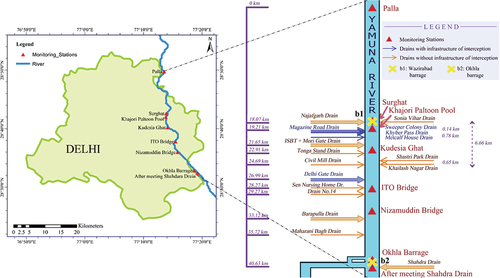
Figure S1 (see Supplementary material) shows a Geographic Information System (GIS) map of New Delhi, highlighting the Yamuna River, the network of drains, industrial zones and common effluent treatment plants (CETPs). It can be reasonably assumed that the discharge from a cluster of neighbouring industries goes into the nearest CETP, and the discharge from these CETPs flows into the nearest drains. A list of various CETPs along with their coordinates is available in Table S3 (see Supplementary material). It is interesting to note that all the CETPs on the left side of the map discharge into the Najafgarh drain, while those on the right side of the map discharge into Shahdara drain. Thus, it can be concluded that barring Najafgarh drain and Shahdara drain, all the drains are expected to carry municipal wastewater only.

3 Data and methods

The present study performs a comprehensive analysis of in situ water quality parameters as well as satellite-derived water quality parameters.

3.1 In situ water quality parameters

Monthly data for four water quality parameters, i.e. pH, BOD, COD, and DO, from 2013 to 2020 at eight in situ monitoring locations over the Delhi-NCT stretch of Yamuna River was extracted from the CPCB website (https://cpcb.nic.in/). Additionally, water quality measurements of pH, COD, BOD, and TSS over the five major discharging drains (Najafgarh, Shahdara, Barapulla, ISBT, Delhi Gate) was extracted for the lean season, i.e. the months of March and April of 2016–2020. Drain water quality data for the year 2019 was missing. It should be noted that the sampling at eight in situ monitoring locations and over drains is performed only on a single day in a month rather than on each individual day of the month.

3.2 Satellite-derived water quality parameters

Four satellite-derived parameters, namely SPM, NDTI, FAI, and NDVI, are considered in this study. They are derived from imagery from the Landsat-8 OLI satellite, which is co-managed by the US National Aeronautics and Space Administration (NASA) and the United States Geological Survey (USGS). Landsat-8 OLI images are freely available from an archive hosted by USGS Earth Explorer. In this study, Landsat-8 OLI Collection 2 data at Level-2 processing was used. Images at Level 2 have been processed with radiometric, geometric, and atmospheric corrections, and hence are “ready-to-use” products (Agapiou 2020). This data is an output of Land Surface Reflectance Code (LaSRC), an atmospheric correction algorithm that resolves the temporal, spatial and spectral effects, and properties of the atmospheric components inherent to top-of-atmosphere (TOA) reflectance. This algorithm utilizes various techniques and data like aerosol inversion tests using the coastal aerosol band, auxiliary climate data from Moderate Resolution Imaging Spectroradiometer (MODIS), etc., to derive surface reflectance values of each band from TOA (Vermote et al. 2016). Landsat-8 OLI images consist of nine spectral bands. However, to derive the four indices considered in this study, only four bands are required, viz. the green band (0.53–0.59 μm), red band (0.64–0.67 μm), near-infrared (NIR) band (0.85–0.88 μm), and shortwave infrared (SWIR) band (2.11–2.29 μm). The data representing each band is the at-sensor reflectance, which are unitless values that have undergone non-linear conversions from initial raw digital numbers (Roy et al. 2014).

The Landsat-8 OLI images are generally available at an interval of 16 days, with the resolution of the different spectral bands being 30 m, barring the Panchromatic (PAN) band, which is available at a resolution of 15 m. In this study, images from the entire Landsat-8 collection (Path: 146, Row: 40) available from May 2013 to August 2021 were considered. From each month, dates with the least amount of cloud cover were chosen. However, images from some months could not be used for the analysis due to excessive cloud cover over the study area. Finally, 50 dates were finalized for analysis (see Supplementary material, Table S4). Google Earth Engine is used to directly access these images from the USGS repository.

SPM was calculated from the red band using an empirical equation derived by Nechad et al. (2010), as shown in Equation (1)(1) $\mathrm{S}\mathrm{P}\mathrm{M}=\frac{\mathrm{A}.{\rho }_{\mathrm{w}}}{1-\left({\rho }_{\mathrm{w}}/\mathrm{C}\right)}+\mathrm{B}$(1) .

(1) $\mathrm{S}\mathrm{P}\mathrm{M}=\frac{\mathrm{A}.{\rho }_{\mathrm{w}}}{1-\left({\rho }_{\mathrm{w}}/\mathrm{C}\right)}+\mathrm{B}$(1)

where ${\rho }_{\mathrm{w}}$ is surface reflectance for the red band; A (289.29), B (0), and C (0.1686) are calibrated coefficients (Nechad et al. 2010). The above equation is only applicable to waters where the SPM levels are below 110 mg/L. It must be noted that ${\rho }_{\mathrm{w}}$ denotes water leaving reflectance, which is given by π multiplied with $R_{rs}$ (remote sensing reflectance). $R_{rs}$ can generally be obtained upon dividing normalized water-leaving radiances with TOA solar irradiance (Ilori et al. 2019). However, as the LaSRC product is presented in terms of the above-surface diffuse reflectance ($R\left(0^{+}\right)$), the following formula can be used to retrieve ${\mathrm{R}}_{\mathrm{r}\mathrm{s}}$:

(2) ${\mathrm{R}}_{\mathrm{r}\mathrm{s}}=\frac{\mathrm{R}\left(0^{+}\right)}{\pi }$(2)

Thus, ${\rho }_{\mathrm{w}}$, given by π multiplied with ${\mathrm{R}}_{\mathrm{r}\mathrm{s}}$, becomes mathematically equivalent to the surface reflectance of red band (${\mathrm{R}}_{\mathrm{r}\mathrm{e}\mathrm{d}}$). SPM is a measure of sediments caused by metal and chemical contaminants in the water body which directly affect the water’s inherent primary production by hindering the propagation of light.

To estimate the turbidity levels, NDTI (Lacaux et al. 2007) was retrieved using Equation (3)(3) $\mathrm{N}\mathrm{D}\mathrm{T}\mathrm{I}=\frac{{\mathrm{R}}_{\mathrm{r}\mathrm{e}\mathrm{d}}-{\mathrm{R}}_{\mathrm{g}\mathrm{r}\mathrm{e}\mathrm{e}\mathrm{n}}}{{\mathrm{R}}_{\mathrm{r}\mathrm{e}\mathrm{d}}+{\mathrm{R}}_{\mathrm{g}\mathrm{r}\mathrm{e}\mathrm{e}\mathrm{n}}}$(3) , utilizing the reflectance of red and green bands.

(3) $\mathrm{N}\mathrm{D}\mathrm{T}\mathrm{I}=\frac{{\mathrm{R}}_{\mathrm{r}\mathrm{e}\mathrm{d}}-{\mathrm{R}}_{\mathrm{g}\mathrm{r}\mathrm{e}\mathrm{e}\mathrm{n}}}{{\mathrm{R}}_{\mathrm{r}\mathrm{e}\mathrm{d}}+{\mathrm{R}}_{\mathrm{g}\mathrm{r}\mathrm{e}\mathrm{e}\mathrm{n}}}$(3)

where ${\mathrm{R}}_{\mathrm{r}\mathrm{e}\mathrm{d}}$ and ${\mathrm{R}}_{\mathrm{g}\mathrm{r}\mathrm{e}\mathrm{e}\mathrm{n}}$ are the surface reflectance of the red band and green band, respectively.

NDTI varies between −1 and +1, with negative values indicating more transparent waters and positive values denoting higher turbidity.

To measure eutrophication, NDVI and FAI (Dogliotti et al. 2018) were used as they indicate vegetation and algal blooms, respectively, which are generally stimulated by nitrogen and phosphorus content in sewage, industrial effluents, and runoff from fertilizers and agricultural activities (Anderson et al. 2007). NDVI is estimated using Equation (4)(4) $\mathrm{N}\mathrm{D}\mathrm{V}\mathrm{I}=\frac{{\mathrm{R}}_{\mathrm{N}\mathrm{I}\mathrm{R}}-{\mathrm{R}}_{\mathrm{r}\mathrm{e}\mathrm{d}}}{{\mathrm{R}}_{\mathrm{N}\mathrm{I}\mathrm{R}}+{\mathrm{R}}_{\mathrm{r}\mathrm{e}\mathrm{d}}}$(4) (Carlson and Ripley 1997):

(4) $\mathrm{N}\mathrm{D}\mathrm{V}\mathrm{I}=\frac{{\mathrm{R}}_{\mathrm{N}\mathrm{I}\mathrm{R}}-{\mathrm{R}}_{\mathrm{r}\mathrm{e}\mathrm{d}}}{{\mathrm{R}}_{\mathrm{N}\mathrm{I}\mathrm{R}}+{\mathrm{R}}_{\mathrm{r}\mathrm{e}\mathrm{d}}}$(4)

where ${\mathrm{R}}_{\mathrm{N}\mathrm{I}\mathrm{R}}$ is the surface reflectance of the near-infrared band.

FAI is computed using Equation (5)(5) $\mathrm{F}\mathrm{A}\mathrm{I}={\mathrm{R}}_{\mathrm{N}\mathrm{I}\mathrm{R}}-\left[\frac{{\mathrm{R}}_{\mathrm{r}\mathrm{e}\mathrm{d}}\left({\lambda }_{\mathrm{N}\mathrm{I}\mathrm{R}}-{\lambda }_{\mathrm{S}\mathrm{W}\mathrm{I}\mathrm{R}}\right)+{\mathrm{R}}_{\mathrm{S}\mathrm{W}\mathrm{I}\mathrm{R}}\left({\lambda }_{\mathrm{r}\mathrm{e}\mathrm{d}}-{\lambda }_{\mathrm{N}\mathrm{I}\mathrm{R}}\right)}{\left({\lambda }_{\mathrm{r}\mathrm{e}\mathrm{d}}-{\lambda }_{\mathrm{S}\mathrm{W}\mathrm{I}\mathrm{R}}\right)}\right]$(5) , formulated by Dogliotti et al. (2018):

(5) $\mathrm{F}\mathrm{A}\mathrm{I}={\mathrm{R}}_{\mathrm{N}\mathrm{I}\mathrm{R}}-\left[\frac{{\mathrm{R}}_{\mathrm{r}\mathrm{e}\mathrm{d}}\left({\lambda }_{\mathrm{N}\mathrm{I}\mathrm{R}}-{\lambda }_{\mathrm{S}\mathrm{W}\mathrm{I}\mathrm{R}}\right)+{\mathrm{R}}_{\mathrm{S}\mathrm{W}\mathrm{I}\mathrm{R}}\left({\lambda }_{\mathrm{r}\mathrm{e}\mathrm{d}}-{\lambda }_{\mathrm{N}\mathrm{I}\mathrm{R}}\right)}{\left({\lambda }_{\mathrm{r}\mathrm{e}\mathrm{d}}-{\lambda }_{\mathrm{S}\mathrm{W}\mathrm{I}\mathrm{R}}\right)}\right]$(5)

where ${\mathrm{R}}_{\mathrm{S}\mathrm{W}\mathrm{I}\mathrm{R}}$ = surface reflectance in the SWIR band;

${\lambda }_{\mathrm{R}\mathrm{E}\mathrm{D}}$ = the central wavelength in the red band (i.e. λ = 655 μm);

${\lambda }_{\mathrm{N}\mathrm{I}\mathrm{R}}$ = the central wavelength in the NIR band (i.e. λ = 865 μm); and

${\lambda }_{\mathrm{S}\mathrm{W}\mathrm{I}\mathrm{R}}$ = the central wavelength in the SWIR band (λ = 1650 μm).

It is noted that the reflectance values must be Rayleigh corrected. The LaSRC algorithm already accounts for this by approximating and correcting the atmosphere’s reflectance due to Rayleigh scattering (Vermote et al. 2018, see also Equation S1). FAI and NDVI vary from −1 to +1. Negative values are indicative of clearer waters, and higher values of NDVI represent vegetation, while high FAI indicates the presence of algal blooms.

3.3 Processing of Landsat-8 images in Google Earth Engine

Google Earth Engine was used to process and plot index maps. The selected images were first overlain with a pre-existing cloud mask made explicitly for Landsat collection, to minimize any interference of clouds when extracting surface reflectance values. An outline of the Yamuna River passing through Delhi NCT was created in Google Earth Engine. To the outline, the NDWI mask was applied to delineate the water body properly (McFeeters 1996). Ideally, setting the NDWI threshold value to 0 is expected to mask non-water pixels, but studies have found that this might not always lead to good accuracy (Xu 2006), and manual adjustment could give better delineation results (Ji et al. 2009). After a series of trials, an NDWI threshold of −0.15 was finalized for this region to detect water pixels accurately to the maximum possible extent. Furthermore, to avoid anomalies, pixels crossing values of 110 mg/L in SPM and those that did not fall in the range of −1 to 1 for other indices were removed. The entire region was divided along the vertical axis into 80 equal segments of ~0.6 km each to observe significant spatial variations. Further, the average index value was mapped at each segment, i.e. each segment now represents the mean of all pixels within it. Thus, the index values were derived, and the resultant index-wise images were downloaded for analysis.

4 Results and discussion

The present analysis considers five in situ observed water quality parameters (pH, COD, BOD, DO, TSS) and four satellite-derived parameters (SPM, NDTI, NDVI, and FAI).

4.1 In situ water quality parameters

4.1.1 Variation of water quality parameters along the river

Figure 2 shows the annual average variation of water quality parameters along the length of the river (derived from eight monitoring stations) for five years (2016–2020). Overall, pH values are well within the expected pH range of surface water. Even though there is a slight decrease in pH when the Najafgarh drain discharges into Yamuna, the pollution load has not resulted in any substantial changes in pH (Fig. 2(a)). A decrease is observed in 2020 compared to 2019 (the year 2019 has the highest values). Figure 2(b) captures the variation in COD down the length of the river. A remarkable jump in magnitude is seen around 18 km from Palla, for all years. Beyond this point, values start to decrease, before jumping again, albeit less than the previous jump, at around 40 km. Additionally, the values in 2016 are on the high side, as compared to 2019. An identical pattern is observed for BOD (indicated in Fig. 2(c)). Discharges from the Najafgarh drain, the largest drain (18.07 km from Palla station), and Shahdara drain (40.63 km from Palla station), the second-largest drain, are responsible for the two consecutive jumps that were observed. Subsequently, in the case of DO, drops are observed at the same points, as indicated in Fig. 2(d). Moreover, DO in 2020 is relatively higher along the majority of the stretch as compared to other years. Therefore, it can be observed that for BOD, COD, and DO, the variations are following their respective patterns across all five years, with minor changes in their respective magnitudes – unlike pH, which shows no specific pattern.

Figure 2. Spatial variation of average water quality parameters – (a) pH, (b) COD, (c) BOD, and (d) DO – along the length of the river for five different years, from 2016 to 2020.

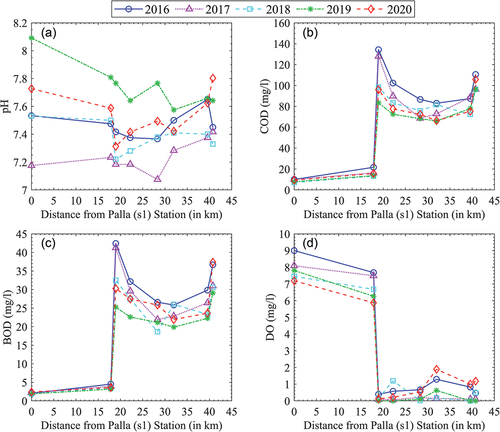
As the 2020 lockdown was imposed for a short duration only (25 March–31 May), the impact of lockdown is not clearly visible in the annual average variation of water quality parameters during 2020 (since the water quality parameters were averaged over the entire year). However, DO values are found to be lowest in 2020 in the initial part of the stretch (indicating the poorest water quality); however, in the later part of the stretch, DO is significantly improved compared to other years. This indicates that the lower pollution load in the lockdown period had a long-term impact in the later part of the stretch, even after the lockdown was lifted.

To further investigate the effect of the 2020 lockdown, monthly variations of water quality parameters during the year 2020 are derived as illustrated in Fig. 3(a–d). Like Fig. 2(a), there is no significant variation in the pH values here either (Fig. 3(a)). A sudden decrease in COD and BOD is observed in April relative to the preceding month, but then there is an increase by June to the same levels that were reached in March (Fig. 3(b) and (c)). This highlights the importance of lockdown in improving water quality, which when lifted in June undid the observed improvements. During July, August and September low values of COD and BOD are observed, probably owing to dilution by monsoon rainfall. Dilution is maximum in the month of August 2020, when the region received the highest rainfall, of 218.4 mm (see Supplementary material, Fig. S2; India-Water Resources Information System (WRIS)). DO also shows a sudden increase in the same monsoon period (Fig. 3(d)). Improvement of DO throughout the stretch is also observed in the lockdown period, as the mean DO shoots up to 2.89 mg/L in April (start of lockdown) as compared to the previous month’s mean value of 1.75 mg/L. It is interesting to note that very little rainfall (10.1 mm) was received during the lockdown phase (April 2020), as compared to the pre-lockdown phase (March 2020), where unseasonal excess rainfall (76 mm) was recorded (see Supplementary material, Fig. S2). Even due to this excess rainfall, the highest BOD and COD were observed in March and then decreased in April. This probably indicates that the improvement in water quality in April largely resulted from lockdown, and possibly was not due to dilution. This is further supported when the DO variation in 2020 (Fig. 3(d)) is compared with that of 2018 and 2019 (see Supplementary material, Fig S3(a) and (b)). High median DO values are observed in 2020, while in 2018 and 2019, they are mostly zero. Mean DO values are also the highest in 2020. This indicates that DO did rejuvenate in 2020 which probably was due to the imposition of lockdown.

Figure 3. The left column presents variation of (a) pH, (b) COD, (c) BOD, and (d) DO within the eight stations for each month of 2020. The right column presents temporal variation of water quality parameters (e) pH, (f) COD, (g) BOD, and (h) DO within the eight stations in April months from 2013 to 2020. Lockdown period was from April to May. Data for May was unavailable. The red line shows the average values in each month over the river stretch. The horizontal line inside each box shows the median. The bottom and top edges of the boxes show the lower and upper quartiles, respectively. Whiskers indicate the highest and lowest values. Small circles represent outliers.

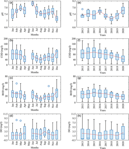
Further, the water quality data records for the month of April over the last eight years (2013–2020) were analysed to precisely investigate the effect of lockdown in April 2020 (see Fig. 3(e–h)). Highly irregular variation in the pH is observed, as shown in Fig. 3(e). COD (Fig. 3(f)) and BOD (Fig. 3(g)) follow a gradually decreasing trend (post 2015), and the lowest values for April are obtained in 2020. DO in 2020 shows the highest April values among all the years (Fig. 3(h)), clearly indicating significant water quality improvement. A decrease in BOD and COD, together with the increase in DO in April of 2020, when compared to the same period in previous years, points to the possible impact of lockdown.

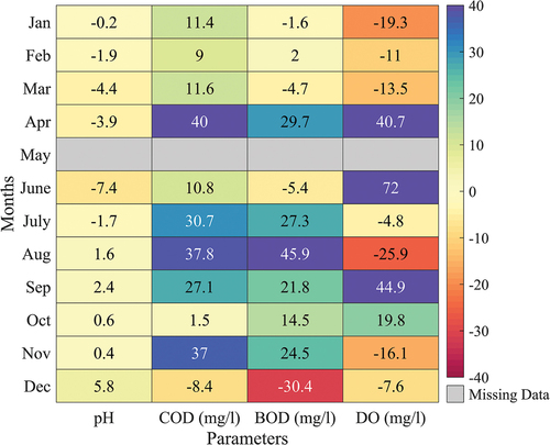
Figure 4 presents the percentage change between the average value of 2013–2019 and 2020 for all in situ parameters in the form of a heat map. Positive percentage variation indicates improvement, whereas a negative value denotes deterioration. Compared to the other three parameters, the average percentage variation in pH is only −0.9%. In contrast, COD, BOD and DO show a high percentage of improvement in April with values of 40%, 29.7% and 40.7%, respectively. As this is seen in the month immediately after lockdown was implemented, this major improvement is possibly due to the impact of lockdown. In June, while BOD (−5.4%) did not undergo any betterment, COD (10.8%) and DO (72%) show good improvement. Moreover, it can be seen that the highest positive variation of all parameters was exhibited by DO in June. This points to the lingering effect of lockdown. An improvement can be seen in all three parameters from July to September, with the exception of DO in July (−4.8%) and August (−25.9%). But as mentioned earlier, any betterment of values seen in the period spanning July, August and September is possibly due to the dilution brought by the monsoon season.

Figure 4. Improvement in water quality parameters (pH, COD, BOD and DOSPM, NDTI, FAI and NDVI) during 2020 considering the average water quality conditions during the 2013 to 2019 period as a reference or baseline.

4.1.2 Variation of water quality parameters in contributing drains

The water quality of five major polluting drains (viz. Najafgarh, ISBT, Delhi Gate, Barapulla, Shahdara) draining to Yamuna, during the lean season months, i.e. March and April, across different years, is illustrated in Fig. S4 (see Supplementary material). Shahdara drain is the most polluting drain as it carries the highest COD, BOD and TSS (see Supplementary material, Fig. S4). Observations reveal that water quality variations vary most vividly in 2020 when compared to other years (comparing the time stamps of the same year). In 2020, the water quality significantly improves from March to April, as indicated in the figure. Barapulla drain does not follow this trend because it mainly carries domestic discharge. Further, it can clearly be seen that the year 2020 does not follow the same pattern as preceding years, indicating that changes in water quality – primarily the improvement in April 2020 – may be due to lockdown.

4.1.3 Comparison with 2021 lockdown

It was stated earlier that Najafgarh drain and Shahdara drain are the prime sources of industrial effluents, and both of these drains show improvements during the lockdown period of 2020. The industrial effluents are captured by CETPs, treated, and then released into the drains. To obtain further insights, the “inlet” data for the various CETPs were compiled and compared across different years. The differences in the CODs for the periods: (i) May 2019–May 2020, and (ii) June 2020–May 2021, were calculated to obtain an idea of the effect of the two lockdowns. It was observed that the difference was non-negative for eight out of 13 CETPs, in both the periods. In fact, similar patterns were observed for BOD and TSS. These observations once again point to the improvements induced due to the lockdown in 2020.

4.2 Satellite-derived water quality parameters

4.2.1 Variation of water quality parameters along the length of the river

Figure 5 presents the spatial variation of SPM, NDTI, FAI and NDVI along the length of the river in the period 2017 to 2020. The spatial variations of SPM (Fig. 5(a)) and NDTI (Fig. 5(b)) are found to be quite similar. Both indices exhibit relatively higher values in the initial part of the stretch, i.e. from Palla to Wazirabad Barrage (b1). As the region around Palla is highly cultivated, it is expected to produce a significant amount of agricultural runoff every year, thus affecting SPM and turbidity (Poudel et al. 2010, FAO 2017). Faster and freer water flow exists in the initial part as there are no drains joining here. This may cause sediment resuspension, resulting in higher SPM. Moreover, possible sediment deposition near b1 due to the restraint provided may also result in higher values (Schmidt et al. 2005). Several drains with an additional pollution load join after b1, as listed in Table S2 (see the Supplementary material). However, after a few kilometres of concentrations similar to that measured at b1, a steady decrease can be seen until b2 (Okhla Barrage). This is because the wastewater carried by all the joining drains is significantly less than that of the first drain, i.e. Najafgarh, giving scope for relative improvement due to the self-cleansing action of the river. Beyond that, the Shahdara drain (second-largest drain) joins, resulting in an increase in SPM and NDTI values. A peculiar thing to note is that SPM and NDTI values were the lowest in 2020 in the stretch beyond b1, i.e. the point at which several drains start joining. This indicates that drains carried less suspended sediment on average when compared to previous years, which could be an effect of lockdown. Thus, SPM and NDTI averaged over the entire year have shown considerable improvements in 2020, despite the short duration of lockdown imposed.

Figure 5. Spatial variation of satellite-derived parameters – (a) SPM, (b) NDTI, (c) FAI and (d) NDVI – along the length of the river in the period from 2017 to 2020. Each line plot comprises 80 points which represent 80 segments of the river and, further, each point represents the average value of its corresponding segment over the entire year.

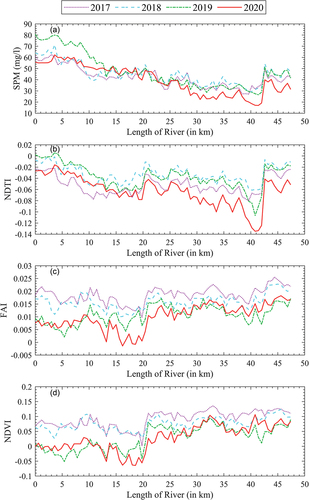
As stated earlier, FAI is an indicator of algal blooms whereas NDVI denotes vegetation cover. Higher values of FAI and NDVI indicate excessive nutrient load released into the river due to agricultural runoff and wastewater discharged through the drains. To flush these out significantly, a velocity of 0.75 m/s (Chow 1973) is required, but the measured average flow velocity of the river is only 0.04 m/s (Soni et al. 2014). Whereas the respective estimated required flow to avoid algal blooms in non-monsoon seasons is 1.8 TMCM, the river stretch falls below this standard with a flow of only 0.44 TMCM (Soni et al. 2014). Thus, it can be concluded that algal blooms and vegetation are expected to be persistent in the river stretch, as revealed by the analysis. Figure 5(c) and (d) presents the levels of FAI and NDVI, respectively, along the stretch. It can be observed that the initial part of the stretch shows slightly lower values. As stated above, this part has a freer flowing capability, and this might lead to slow dispersal of vegetation into the latter area of the river stretch. Thus, algal blooms and vegetation are relatively more persistent in the latter part of the stretch.

4.2.2 Spatial variation of water quality parameters over the entire river stretch

Any change in water quality during the lockdown period could also be attributed to yearly trends. To eliminate this possibility, the variations of SPM, NDTI, NDVI and FAI across the years for relevant dates in the months of March, April, and May, along with the post-lockdown month of June, were analysed.

Figure 6 shows the segment-wise averaged spatiotemporal variation of SPM for each month, with the values ranging from 0 mg/L (blue) to 110 mg/L (red). From Fig. 6(a), it can be observed that 2015 and 2020 exhibited comparatively higher values in March. Most of these levels occurred in the stretch around and before b1. In April (Fig. 6(b)), levels in the region upstream of b1 gradually worsened from 2017 to 2020, while the rest of the stretch did not show major variation. The month of May (Fig. 6(c)) in 2020 showed noticeably lower levels (0 to 20 mg/L) in many parts of the region downstream of b1. In June 2020 (Fig. 6(d)), the stretch below b1 exhibited levels that were on par with the previous year’s levels. Additionally, a notable improvement can be seen in the stretch upstream of b1. Similar patterns were exhibited by NDTI for each month, as shown in Fig. S5 (see Supplementary material).

Figure 6. Segment-wise mean values for SPM in (a) March, (b) April, (c) May, and (d) June across different years. Points b1 and b2 denote the location of Wazirabad barrage and Okhla barrage, respectively.

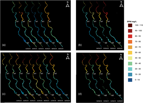
Figure S6 (see Supplementary material) shows the corresponding box-and-whisker plots of SPM and NDTI. Figure S6(a) and (b) follow the above observations made for SPM in March and April. But a few more key observations can be made from the box-and-whisker plots for May and June. Unlike the corresponding spatiotemporal inference made from May, an obvious decrease in levels in 2020 cannot be observed from Fig. S6(c). This is because box-and-whisker plots consider the river stretch in its entirety and higher values seen in some parts overshadow any significant improvements observed. From Fig. S6(d) for June, it can be seen that 2020 showed significantly lower values, with its mean value falling from the preceding 2019 observation. Upon analysis of NDTI, apart from slight differences, it can be seen that it largely conformed to the pattern exhibited by SPM. NDTI also exhibited higher values in March 2020 (Fig. S6(e)). But Fig. S6(f) for April shows a drop in mean NDTI of 2020 when compared to 2019. In May (Fig. S6(g)), a steady decline can be seen only after 2017, with the values in 2020 going as low as −0.16. June (Fig. S6(h)) again showed a pattern similar to that of SPM, as 2020 showed a drop in values.

In the initial lockdown stage of March, SPM and NDTI levels showed no betterment, but as 29 March 2020 is just four days after the lockdown was imposed, an immediate effect cannot be expected. A CPCB report (CPCB 2022) stated that there was a spike in water inflow from Wazirabad Barrage in the latter part of March that gave rise to faster-flowing waters on 29 March, which could have led to sediment resuspension and thus an increase in SPM and NDTI values. The effect of lockdown is clearly evident only in the months of May and June. In May, high values seen in the Palla region overshadow the improvements observed in the rest of the stretch. Thus, if we consider only the region below b1 for our analysis, the impact of lockdown is quite apparent. While the improvement is only by a factor of 10 mg/L at most, it can be concluded from an inspection of segment-wise averaged maps that this part of the stretch recorded the lowest levels in eight years, for both indices. This can be seen especially in reaches around Okhla region. Moreover, the post-lockdown month of June also showed lower values compared to the previous year.

Figure 7 illustrates the segment-wise averaged maps of FAI. FAI for this study area exhibited a range of −0.04 to 0.06. From Fig. 7(a), it can be observed that 29 March showed very low values throughout the stretch. In April (Fig. 7(b)), the values along the stretch from 2017 to 2020 were similar. May (Fig. 7(c)), 2020 showed the lowest FAI levels in the period considered and June 2020 (Fig. 7(d)) showed lower values in the stretch upstream of b1. Similar patterns were observed in spatiotemporal variation of NDVI for each month as shown in Fig. S7 (see Supplementary material).

Figure 7. Segment-wise mean values for FAI in (a) March, (b) April, (c) May, and (d) June across different years. Points b1 and b2 denote the location of Wazirabad barrage and Okhla barrage, respectively.

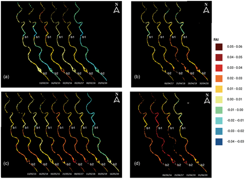
Figure S8(a–d) (see Supplementary material) presents the box-and-whisker plots of FAI. Further adding to the previously observed abnormal values in March 2020, it can be inferred from Fig. S8(a) that these were in fact the lowest observed since 2014. In April, the variations shown in Fig. S8(b) are too small to be of any significance. In accordance with the inference made from Fig. S6(c) previously, Fig. S8(c)) presents further evidence that May 2020 exhibited the lowest values. In June, an overall decline from 2019 is observed. Box-and-whisker plots for NDVI are shown in Fig. S8(e–h) (see Supplementary material). Fig. S8(e) and Fig. S8(f), for March and April, respectively, follow the same pattern as FAI. In May (Fig. S8(g)), a high uniformity of levels is exhibited from 2013 to 2019, with a significant drop in 2020. Like FAI in June, NDVI also showed lower values in 2020 when compared to 2019 (Fig. S8(h)).

The unexpectedly low values of FAI and NDVI in March of 2020 can be attributed to a combination of factors. As mentioned earlier, higher water flow was observed on 29 March 2020. This was coupled with a rapid reduction in anthropogenic and industrial activities due to the sudden imposition of 2020 lockdown. As documented earlier, this stretch is expected to have persistent vegetation and algal blooms, but this increase in water inflow could have contributed to an easy flushing out of such accumulations. This explains the major decrease in values. We can again observe a significant drop in May of 2020 with both the FAI and NDVI levels being the lowest seen in eight years. While the low values in the region downstream of b1 could again be due to a possible higher water inflow, it must be noted that the region upstream showed remarkable improvements. This can be attributed only to the impact of lockdown as Palla region is polluted mainly by domestic and industrial discharge from Sonipat District of Haryana (CPCB 2006), and lockdown would have significantly reduced this activity. In June, while the improvement was not as significant, it is still interesting to note that there was slight betterment post lockdown.

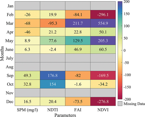
A heat map similar to the one created for in situ parameters has also been made for the four satellite-derived parameters, as shown in Fig. 8. SPM and NDTI are seen to follow a similar pattern. In May, improvements of 8.9% and 77.6% were exhibited by SPM and NDTI, respectively. A decrease in this variation was then seen in June, but SPM (6.3%) still showed an improvement while NDTI (−2.4%) had a low percentage of deterioration. FAI and NDVI can also be seen to follow similar patterns. Significantly better FAI and NDVI values can be seen in March, with improvements of 211.7% and 554.9%, respectively. After a decrease in percentage variation in April, a rise can be seen in May followed by a fall in June. Despite this fluctuating pattern in percentage variation, it can be observed that FAI and NDVI had better values in 2020 for the months of March, April, May, and June, i.e. for the entire duration of the pre-lockdown, lockdown and post-lockdown periods.

Figure 8. Improvement in water quality parameters (SPM, NDTI, FAI and NDVI) during 2020 considering the average water quality conditions during the 2013 to 2019 period as reference or baseline.

4.2.3 Relationship between different satellite-derived water quality parameters

It has been repeatedly observed that the pairs SPM-NDTI and FAI-NDVI follow a similar pattern. To verify these observations and remove any subjective bias due to visual inspection, density-scatter plots were created (see Supplementary material, Fig. S9). A direct relationship can be seen between the two pairs (SPM-NDTI and FAI-NDVI), and they exhibited Pearson’s correlation coefficient values of 0.71 (Fig. S9(d)) and 0.91 (Fig. S9(f)), respectively. Other combinations exhibited very low correlation values. The relation between SPM and NDTI can be justified as suspended particles may affect the turbidity of the water too. A few studies have also tried to investigate this and established a mathematical correlation between the two parameters (Jafar-Sidik et al. 2017). Similarly, as NDVI and FAI can be used to indicate the same phenomenon of eutrophication, they are expected to exhibit good correlation. This inference was also noted in a previous study (Visitacion et al. 2019). The correlation analysis done in this study verifies these facts, and also confirms that the correlation holds true in the study area under consideration.

4.2.4 Dependence of satellite-derived water quality parameters on rainfall

Upon further investigating the trends of SPM, it was observed that the recorded SPM values show a temporary jump during the months that experienced a decent amount of rainfall. A similar observation was made by Robert et al. (2017). In this study, a comparison was made between the actual rainfall data (monthly average), and the satellite-derived SPM values averaged over the whole stretch to verify the visual interpretations. Similar comparisons were done with other indices too (see Supplementary material, Fig. S10). It was observed that in most cases, whenever there is a peak in the rainfall pattern, there is also a peak in the SPM values (Fig. 10(a)). The Pearson correlation coefficient was 0.29, which is highest among the other parameters (Fig. S10(b–d)). The influence of rainfall on SPM values is higher than on other parameters, as there is a possibility of increased sediment erosion and transportation during heavy rainfalls. This is caused by an increase in turbulence due to the rising flow velocity and water levels in the river. Moreover, rainfall also leads to surface runoff, thereby acting as an additional temporary source of pollution. As these extra sediments will take a certain amount of time to settle, SPM values can rise temporarily.

4.2.5 Comparison with 2021 lockdown

As observed in the previous sections that dealt with the analysis of satellite-derived indices, the effect of lockdown is clearly visible only a month from its date of imposition. Expecting the same in 2021, we analysed the satellite data available in the latter part of May to see if there were any improvements. The SPM map of 26 May 2021 (see Supplementary material, Fig. S11(a)) showed little to no change compared to the pre-lockdown date of 8 April 2021. Further, we also noted that SPM stayed in the same range of values from April to July, i.e. there was an almost constant trend throughout the periods of pre-lockdown, lockdown, and post-lockdown. This observation is expected as the 2021 lockdown phase was not as restrictive as that of 2020. A similar inference was drawn from the FAI maps (see Supplementary material, Fig. S11(c)). From the analysis of maps from 2013 to 2019, we noted that 2021 was, in fact, simply exhibiting the levels usually expected in the months of May and June. Thus, it is unlikely that the slight changes seen were due to lockdown. We conclude that while 2020 showed remarkable improvements, 2021 had no discernible changes that could be attributed to the effect of lockdown.

5 Conclusions

The following points summarize the inferences of this study:

• Lockdown in 2020 improved BOD and COD in the short term, while DO improved over the long term. Despite the 2020 lockdown, BOD and COD values along the river were not the lowest from 2016 to 2020. DO showed the most growth in 2020, in the latter part of the stretch.

• Wazirabad Barrage to Okhla Barrage had the lowest SPM and NDTI values in eight years in May 2020. FAI and NDVI show the same improvement throughout the stretch.

• SPM and NDTI are highly correlated. Visually inspecting turbidity helps estimate SPM. This is helpful in practice, i.e. performing laboratory tests for SPM should not be necessary when studying water quality qualitatively. Similarly, FAI and NDVI are correlated.

• The average wastewater discharged into the river on a business-as-usual day is around 3026 MLD, and this value dropped by 36 MLD during the lockdown period (CPCB 2022). Industrial effluents contribute 1.18% of total wastewater volume, but their absence reduces COD by 40% and BOD by 29.7%. Many industries are not linked with CETPs and dump their wastewater into drains (Hindustan Times 2022).

• The analysis of inlet CETP data reveals that May 2020 values were lower, compared to June 2021, both of which happen to be indicative of lockdown phases in the two years. Drastic improvements were observed in 2020 which coincided with the hard lockdown; however, no significant improvements were observed in 2021 as the lockdown at that time was not as restrictive and industries remained operational. The fact that CETPs are carrying industrial wastewater only provides evidence that the main source of improvement in water quality has been due to a reduction in industrial effluents. Higher discharge in the river improves water quality by lowering COD & BOD and increasing DO. Further, these improvements are more sensitive to discharge towards the region downstream of the Wazirabad Barrage. This was validated by calculating correlation coefficients between discharge and water quality parameters at Palla and Delhi Railway Bridge (see Supplementary material, Table S5). To further ascertain that these improvements are not due to an increase in the flow of the river itself, the long-term trends in the river flow at Palla and Wazirabad was analysed. The data was sourced from the Central Water Commission (CWC) and is presented in Fig. S12 (see Supplementary material). It was observed that the flow decreased on a year-to year basis. Thus, the alternative possibility does not hold merit.

Water quality in the Delhi-NCT segment of the Yamuna River is significantly affected by the operation of the Wazirabad Barrage and water diversion from the main Yamuna channel. During the monsoon months (July to September), 80% of flow is released, while during the other nine months, only 20% is released (Soni et al. 2014), which negatively impacts the river’s self-cleaning capacity. Further, the average flow velocity near the Wazirabad Barrage is insufficient to flush out contaminants and check algal growth. Additionally, barrage disruptions promote the lotic environment, which moves downstream with the released water and adds to river pollution (Mishra 2010).

Remote sensing may overestimate or underestimate water quality. A lack of in situ data prevented validation in this study. Still, for the sake of comparison, the estimates are reasonable, as has been validated by several studies in the past. Future studies may use high-resolution satellite data instead of Landsat-8 OLI data. Further comparisons can be made between various satellites like Landsat-8, Sentinel-2 and other high-resolution satellites. Ammonia, nitrate, phosphate, total dissolved solids, faecal coliforms, chlorophyll-a, and heavy metals can be studied to achieve a much broader view of the water quality.

This paper examines industrial wastewater’s impact on water quality, indicating that common pollution-reduction strategies can reduce river pollution if implemented properly. To improve the water quality in one of the country’s most polluted rivers, existing frameworks must be redesigned and properly regulated, STPs and CETPs must be properly managed, and existing infrastructures must be upgraded (Gautam et al. 2013). Because the conceptual framework used in this paper can be continuously implemented on any surface water body, the current study will be useful in planning appropriate rejuvenation measures and sustainable management of surface water resources.

Acknowledgements

The authors thank (1) the Central Pollution Control Board, India, for providing the in situ water quality data; (2) the Central Water Commission for providing flow data; and (3) the NASA Goddard Earth Space Flight Center and the United States Geological Survey (https://www.usgs.gov/) for providing the Landsat-8 dataset. We also thank Google Earth Engine for providing a platform to load the dataset, compute indices and analyse the images.

Disclosure statement

No potential conflict of interest was reported by the authors.

Supplementary material

Supplemental data for this article can be accessed online at https://doi.org/10.1080/02626667.2023.2224004

Additional information

Funding

The authors express sincere gratitude to the Indian Institute of Technology Delhi, India, for supporting this work by providing Summer Undergraduate Research Awards (SURA 2021) to Saghan Yadav and Gurpinder Singh. Further, the authors are grateful to the Indian Academy of Sciences (IASc), Indian National Science Association (INSA), and National Academy of Sciences India (NASI), for jointly sponsoring the Summer Research Fellowship Program (2021) for Likhita Nelapudi. The work was also partially supported by funds received from the Global Challenges Research Fund, UK Research & Innovation (Grant Number: ES/S008179/1) for the project “Water Security and Sustainable Development Hub.”

References

- Agapiou, A., 2020. Evaluation of Landsat 8 OLI/TIRS level-2 and sentinel 2 level-1C fusion techniques intended for image segmentation of archaeological landscapes and proxies. Remote Sensing, 12 (3), 579. doi:10.3390/rs12030579
- Anderson, M.C., et al., 2007. A climatological study of evapotranspiration and moisture stress across the continental United States based on thermal remote sensing: 2. Surface moisture climatology. Journal of Geophysical Research: Atmospheres, 112 (D11). doi:10.1029/2006JD007506
- Anderson, D.M., Glibert, P.M., and Burkholder, J.M., 2002. Harmful algal blooms and eutrophication: nutrient sources, composition, and consequences. Estuaries, 25 (4), 704–726. doi:10.1007/BF02804901
- Awoke, A., et al., 2016. River water pollution status and water policy scenario in Ethiopia: raising awareness for better implementation in developing countries. Environmental Management, 58 (4), 694–706. doi:10.1007/s00267-016-0734-y
- Bierman, P., et al., 2011. A review of methods for analysing spatial and temporal patterns in coastal water quality. Ecological Indicators, 11 (1), 103–114. doi:10.1016/j.ecolind.2009.11.001
- Boretti, A. and Rosa, L., 2019. Reassessing the projections of the world water development report. NPJ Clean Water, 2 (1), 1–6. doi:10.1038/s41545-019-0039-9
- Carlson, T.N. and Ripley, D.A., 1997. On the relation between NDVI, fractional vegetation cover, and leaf area index. Remote Sensing of Environment, 62 (3), 241–252. doi:10.1016/S0034-4257(97)00104-1
- Chakraborty, B., et al., 2021a. Positive effects of COVID-19 lockdown on river water quality: evidence from River Damodar, India. Scientific Reports, 11 (1), 1–16. doi:10.1038/s41598-021-99689-9
- Chakraborty, B., et al., 2021b. Cleaning the river Damodar (India): impact of COVID-19 lockdown on water quality and future rejuvenation strategies. Environment, Development and Sustainability, 23 (8), 11975–11989. doi:10.1007/2Fs10668-020-01152-8
- Chakraborty, B., et al., 2021c. Eco-restoration of river water quality during COVID-19 lockdown in the industrial belt of eastern India. Environmental Science and Pollution Research, 28 (20), 25514–25528. doi:10.1007/s11356-021-12461-4
- Chakraborty, B., et al., 2022. Effects of COVID-19 lockdown and unlock on the health of tropical large river with associated human health risk. Environmental Science and Pollution Research, 29 (24), 37041–37056. doi:10.1007/s11356-021-17881-w
- Chaudhary, S., et al., 2019. Water quality–based environmental flow under plausible temperature and pollution scenarios. Journal of Hydrologic Engineering, 24 (5), 05019007. doi:10.1061/(ASCE)HE.1943-5584.0001780
- Chaudhary, S., et al., 2020. Closure to “Water quality–based environmental flow under plausible temperature and pollution scenarios” by Shushobhit Chaudhary, CT Dhanya, Arun Kumar, and Rehana Shaik. Journal of Hydrologic Engineering, 25 (6), 07020005. doi:10.1061/(ASCE)HE.1943-5584.0001914
- Chaudhary, S., Dhanya, C.T., and Kumar, A., 2018. Sequential calibration of a water quality model using reach-specific parameter estimates. Hydrology Research, 49 (4), 1042–1055. doi:10.2166/nh.2017.246
- Chow, V.T., 1973. Open channel hydraulics. New York: McGraw-Hill.
- CPCB (Central Pollution Control Board), 2011. Polluted River stretches in India: criteria and status. Delhi, India: CPCB. Available from: https://cpcb.nic.in/wqm/RS-criteria-status.pdf [Accessed 12 Jun 2022].
- CPCB Report 2006, (ADSORBS/41/2006-07). Water quality status of Yamuna River (1999–2005). Available from: https://yamunariverproject.wp.tulane.edu/wp-content/uploads/sites/507/2021/01/cpcb_2006-water-quality-status.pdf [ Accessed 12 Jun 2022].
- CPCB Report 2020, (MINARS/38/2020-21). Assessment of impact of lockdown on water quality of major rivers. Available from: https://cpcb.nic.in/upload/Assessment-of-Impact-Lockdown-WQ-MajorRivers.pdf [Accessed 12 Jun 2022].
- Currell, M.J. and Han, D., 2017. The global drain: why China’s water pollution problems should matter to the rest of the world. Environment: Science and Policy for Sustainable Development, 59 (1), 16–29. doi:10.1080/00139157.2017.1252605
- Dogliotti, A.I., et al., 2015. A single algorithm to retrieve turbidity from remotely-sensed data in all coastal and estuarine waters. Remote Sensing of Environment, 156, 157–168. doi:10.1016/j.rse.2014.09.020
- Dogliotti, A.I., et al., 2018. Detecting and quantifying a massive invasion of floating aquatic plants in the Rio de la Plata turbid waters using high spatial resolution ocean color imagery. Remote Sensing, 10 (7), 1140. doi:10.3390/rs10071140
- DPCC, 2020. Assessment of Yamuna river water quality Delhi during lockdown period, Delhi pollution control committee. Available from: https://yamuna-revival.nic.in/wp-content/uploads/2020/04/Water-Quality-of-River-Yamuna-during-the-Lockdown.21.04.2020.pdf [ Accessed 12 Jun 2022].
- Dwivedi, S., Mishra, S., and Tripathi, R.D., 2018. Ganga water pollution: a potential health threat to inhabitants of Ganga basin. Environment International, 117, 327–338. doi:10.1016/j.envint.2018.05.015
- FAO, 2017. Water pollution from agriculture: a global review. rome, food and agriculture organization of the United Nations (FAO). Available from: Water pollution from agriculture: a global review - Executive summary (fao.org) [ Accessed 12 Jun 2022].
- Gautam, S.K., et al., 2013. A study of the effectiveness of sewage treatment plants in Delhi region. Applied Water Science, 3 (1), 57–65. doi:10.1007/s13201-012-0059-9
- Glasgow, H.B., et al., 2004. Real-time remote monitoring of water quality: a review of current applications, and advancements in sensor, telemetry, and computing technologies. Journal of Experimental Marine Biology and Ecology, 300 (1–2), 409–448. doi:10.1016/j.jembe.2004.02.022
- Hafeez, S., et al., 2019. Comparison of machine learning algorithms for retrieval of water quality indicators in case-II waters: a case study of Hong Kong. Remote Sensing, 11 (6), 617. doi:10.3390/rs11060617
- Hindustan Times. 910 industries in Delhi fined by government for toxic effluents in drains. Available from: https://www.hindustantimes.com/delhi-news/in-a-first-910-industries-in-delhi-fined-by-government-for-toxic-effluents-in-drains/story-BUbRDtCHO5eqE6lUeDESZN.html [ Accessed 12 Jun 2022].
- Ilori, C.O., Pahlevan, N., and Knudby, A., 2019. Analyzing performances of different atmospheric correction techniques for Landsat 8: application for coastal remote sensing. Remote Sensing, 11 (4), 469. doi:10.3390/rs11040469
- India-WRIS: Rainfall. Available from: India-WRIS (indiawris.gov.in) [ Accessed 12 Jun 2022].
- Jafar-Sidik, M., et al., 2017. The relationship between suspended particulate matter and turbidity at a mooring station in a coastal environment: consequences for satellite-derived products. Oceanologia, 59 (3), 365–378. doi:10.1016/j.oceano.2017.04.003
- Jaiswal, R.K., 2007. Ganga action plan–a critical analysis. Kanpur: Eco Friends. Available from: Mimeo(https://ecofriends.org/main/eganga/images/critical%20analysis%20of%20gap.pdf) [Accessed 14 Jun 2022].
- Jamwal, P., Mittal, A.K., and Mouchel, J.M., 2011. Point and non-point microbial source pollution: a case study of Delhi. Physics and Chemistry of the Earth, Parts A/B/C, 36 (12), 490–499. doi:10.1016/j.pce.2008.09.005
- Ji, L., Zhang, L., and Wylie, B., 2009. Analysis of dynamic thresholds for the normalized difference water index. Photogrammetric Engineering and Remote Sensing, 75 (11), 1307–1317. doi:10.14358/PERS.75.11.1307
- Kour, G., et al., 2021. Impact assessment on water quality in the polluted stretch using a cluster analysis during pre-and COVID-19 lockdown of Tawi river basin, Jammu, North India: an environment resiliency. Energy, Ecology and Environment, 1-12. doi:10.1007/s40974-021-00215-4
- Lacaux, J.P., et al., 2007. Classification of ponds from high-spatial resolution remote sensing: application to Rift Valley Fever epidemics in Senegal. Remote Sensing of Environment, 106 (1), 66–74. doi:10.1016/j.rse.2006.07.012
- Liu, D., et al., 2022. COVID-19 lockdown improved river water quality in China. Science of the Total Environment, 802, 149585. doi:10.1016/j.scitotenv.2021.149585
- McFeeters, S.K., 1996. The use of the Normalized Difference Water Index (NDWI) in the delineation of open water features. International Journal of Remote Sensing, 17 (7), 1425–1432. doi:10.1080/01431169608948714
- Meybeck, M., 2002. Riverine quality at the anthropocene: propositions for global space and time analysis, illustrated by the Seine River. Aquatic Sciences, 64 (4), 376–393. doi:10.1007/PL00012593
- Misra, A.K., 2010. A river about to die: Yamuna. Journal of Water Resource and Protection, 2 (5), 489. doi:10.4236/jwarp.2010.25056
- Nechad, B., Ruddick, K.G., and Park, Y., 2010. Calibration and validation of a generic multisensor algorithm for mapping of total suspended matter in turbid waters. Remote Sensing of Environment, 114 (4), 854–866. doi:10.1016/j.rse.2009.11.022
- Niroumand-Jadidi, M., et al., 2020. Physics-based bathymetry and water quality retrieval using planetscope imagery: impacts of 2020 COVID-19 lockdown and 2019 extreme flood in the Venice Lagoon. Remote Sensing, 12 (15), 2381. doi:10.3390/rs12152381
- Oki, T. and Kanae, S., 2006. Global hydrological cycles and world water resources. Science, 313 (5790), 1068–1072. doi:10.1126/science.1128845
- Patel, P.P., Mondal, S., and Ghosh, K.G., 2020. Some respite for India’s dirtiest river? Examining the Yamuna’s water quality at Delhi during the COVID-19 lockdown period. Science of the Total Environment, 744, 140851. doi:10.1016/j.scitotenv.2020.140851
- Peterson, K.T., et al., 2018. Suspended sediment concentration estimation from landsat imagery along the lower Missouri and middle Mississippi Rivers using an extreme learning machine. Remote Sensing, 10 (10), 1503. doi:10.3390/rs10101503
- Peterson, K.T., Sagan, V., and Sloan, J.J., 2020. Deep learning-based water quality estimation and anomaly detection using Landsat-8/Sentinel-2 virtual constellation and cloud computing. GIScience & Remote Sensing, 57 (4), 510–525. doi:10.1080/15481603.2020.1738061
- Postel, S.L., 2000. Entering an era of water scarcity: the challenges ahead. Ecological Applications, 10 (4), 941–948. doi:10.1890/1051-0761(2000)010[0941:EAEOWS]2.0.CO;2
- Poudel, D.D., Jeong, C.Y., and DeRamus, A., 2010. Surface run-off water quality from agricultural lands and residential areas. Outlook on Agriculture, 39 (2), 95–105. doi:10.5367/000000010791745394
- Robert, E., et al., 2017. Analysis of suspended particulate matter and its drivers in Sahelian ponds and lakes by remote sensing (Landsat and MODIS): Gourma region, Mali. Remote Sensing, 9 (12), 1272. doi:10.3390/rs9121272
- Roy, D.P., et al., 2014. Landsat-8: science and product vision for terrestrial global change research. Remote Sensing of Environment, 145, 154–172. doi:10.1016/j.rse.2014.02.001
- Said, S. and Hussain, A., 2019. Pollution mapping of Yamuna River segment passing through Delhi using high-resolution GeoEye-2 imagery. Applied Water Science, 9 (3), 1–8. doi:10.1007/s13201-019-0923-y
- Sarkar, S., et al., 2021. Effects of COVID-19 lockdown and unlock on health of Bhutan-India-Bangladesh trans-boundary rivers. Journal of Hazardous Materials Advances, 4, 100030. doi:10.1016/j.hazadv.2021.100030
- Schmidt, A., et al., 2005. Investigations to reduce sedimentation upstream of a barrage on the river Rhine. WIT Transactions on Ecology and the Environment, 80. Available from: https://www.witpress.com/Secure/elibrary/papers/WRM05/WRM05015FU.pdf [Accessed 14 Jun 2022].
- Schwarzenbach, R.P., et al., 2010. Global water pollution and human health. Annual Review of Environment and Resources, 35 (1), 109–136. doi:10.1146/annurev-environ-100809-125342
- Sharma, D. and Kansal, A., 2011. Water quality analysis of River Yamuna using water quality index in the national capital territory, India (2000–2009). Applied Water Science, 1 (3), 147–157. doi:10.1007/s13201-011-0011-4
- Soni, V., Shekhar, S., and Singh, D., 2014. Environmental flow for the Yamuna river in Delhi as an example of monsoon rivers in India. Current Science, 558–564. Available from: https://www.jstor.org/stable/24100063 [Accessed 14 Jun 2022].
- Tokatlı, C. and Varol, M., 2021. Impact of the COVID-19 lockdown period on surface water quality in the Meriç-Ergene River Basin, Northwest Turkey. Environmental Research, 197, 111051. doi:10.1016/j.envres.2021.111051
- Vermote, E., et al., 2016. Preliminary analysis of the performance of the Landsat 8/OLI land surface reflectance product. Remote Sensing of Environment, 185, 46–56. doi:10.1016/j.rse.2016.04.008
- Vermote, E., et al., 2018. LaSRC (Land Surface Reflectance Code): overview, application and validation using MODIS, VIIRS, LANDSAT and Sentinel 2 data’s. In: IGARSS 2018-2018 IEEE International Geoscience and Remote Sensing Symposium, Valencia, Spain. IEEE, 8173–8176. Available from: https://ieeexplore.ieee.org/document/8517622 [Accessed 3 Jul 2023].
- Visitacion, M.R., et al., 2019. Detection of algal bloom in the coastal waters of boracay, Philippines using normalized difference vegetation index (ndvi) and floating algae index (FAI). International Archives of the Photogrammetry, Remote Sensing & Spatial Information Sciences, XLII-4/W19, 479–486. doi:10.5194/isprs-archives-XLII-4-W19-479-2019
- Wagh, P., et al., 2020. Indicative lake water quality assessment using remote sensing images-effect of COVID-19 lockdown. Water, 13 (1), 73. doi:10.3390/w13010073
- Walling, B., et al., 2017. Estimation of environmental flow incorporating water quality and hypothetical climate change scenarios. Environmental Monitoring and Assessment, 189 (5), 225. doi:10.1007/s10661-017-5942-2
- Wang, X., Zhang, F., and Ding, J., 2017. Evaluation of water quality based on a machine learning algorithm and water quality index for the Ebinur Lake Watershed, China. Scientific Reports, 7 (1), 1–18. doi:10.1038/s41598-017-12853-y
- Xing, Y., et al., 2005. A spatial temporal assessment of pollution from PCBs in China. Chemosphere, 60 (6), 731–739. doi:10.1016/j.chemosphere.2005.05.001
- Xu, H., 2006. Modification of normalised difference water index (NDWI) to enhance open water features in remotely sensed imagery. International Journal of Remote Sensing, 27 (14), 3025–3033. doi:10.1080/01431160600589179
- YMC, 2019. Yamuna monitoring committee report. Available from: https://yamuna-revival.nic.in/wp-content/uploads/2019/02/Pollution-of-the-River-Yamuna.pdf [ Accessed 12 Jun 2022].
- YMC, 2020. Yamuna monitoring committee report. Available from: Final-Report-of-YMC-29.06.2020.pdf (Yamuna-revival.nic.in) [ Accessed 12 Jun 2022].
- Yunus, A.P., Masago, Y., and Hijioka, Y., 2020. COVID-19 and surface water quality: improved lake water quality during the lockdown. Science of the Total Environment, 731, 139012. doi:10.1016/j.scitotenv.2020.139012
- Zhao, S., et al., 2005. The 7-decade degradation of a large freshwater lake in Central Yangtze River, China. Environmental Science & Technology, 39 (2), 431–436. doi:10.1021/es0490875