Automatic water-level class estimation from repeated crowd-based photos of streams

ABSTRACT

Citizen science projects engage the public in monitoring the environment and can collect useful data. One example is the CrowdWater project, in which stream levels are observed and compared to reference photos taken at an earlier time to obtain stream level class data. However, crowd-based observations are uncertain and require data quality control. Therefore, we used a deep learning model to estimate the water-level class for photos taken by citizen scientists at different times for the same stream and compared different options for model training. The models had a root mean square error (R) of 0.5 classes or better for all but four of the 385 sites for which the model was trained. Low water levels were in general predicted better than high water levels (R of 0.6 vs 1.0 classes). The study thus highlights the potential of human–computer interaction for data collection and quality control in citizen science projects.

KEYWORDS:

• citizen science
• deep learning
• water-level class
• stream

Editor R. Singh; Associate Editor (not assigned)

1 Introduction

Hydrological models commonly used in water resource management need at least some data to be adapted or calibrated for the target catchment. Observations (i.e. data) are thus required before these models can be used to predict floods and droughts, or the impacts of climate change. However, for many locations, observations are missing due to the high installation and maintenance costs of long-term streamflow gauging stations (Fekete et al. 2012, Ruhi et al. 2018). This is especially true for small headwater streams (Kirchner 2006) and developing countries (Mulligan 2013).

New observational approaches, such as remote sensing and time-lapse cameras, can supplement the data from hydrometric networks and help to better understand hydrological processes and improve water resources management (Tauro et al. 2018). However, acquiring data of high spatial–temporal resolution in real time or over the long term is still challenging. By engaging the public in data collection, citizen science projects can potentially address the pressing need for high-quality data in hydrological research (Assumpção et al. 2018, Njue et al. 2019). Not only does citizen science data contribute to hydrological monitoring and mapping (Smith et al. 2017, Li et al. 2018, Fritz et al. 2019), it also can be integrated into hydrological models to enhance model performances (Yu et al. 2016, Mazzoleni et al. 2017, Weeser et al. 2018, Annis and Nardi 2019). Incorporating more citizen science research into constructing and training data-driven models can, similarly, improve hydrological observations (Gómez et al. 2021).

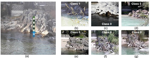
Citizen science projects employ diverse methods for data collection. Some projects provide low-cost monitoring equipment for people (Walker et al. 2016, Starkey et al. 2017) or install staff gauges and ask people to submit the water level via an SMS message (Weeser et al. 2018, Lowry et al. 2019). Other citizen science projects aim to identify whether floods occur or investigate specific flood or drought events (Le Coz et al. 2016). In the CrowdWater project (Seibert et al. 2019), long-term water level data can be collected by citizen scientists via a mobile phone application (app). These observations do not require any physical installations and are based on a comparison of the current water level to the water level at a previous time. An image of a staff gauge is digitally inserted into a photo of a static reference object, such as a stream bank, bridge pillar, or pile of rocks (Fig. 1(a)). This reference image with the virtual staff gauge is used to compare the water level during subsequent visits by the same or another citizen scientist to determine the water-level class at different times (Fig. 1(b)–(g)). This way, time series of water-level class data can be obtained.

Figure 1. Photographs illustrating the principle of the virtual staff gauge approach used in the CrowdWater project. The first observer at a location (i.e. spot) takes a photo that shows the water surface and a reference object (in this case a pile of rocks) and inserts the virtual staff gauge (a sticker) in the photo, in such a way that class 0 (blue line) is on the water surface (a). The same observer or other observers can take photos of the spot at a later time and determine the new water-level class by looking at the position of the water surface relative to the reference objects (b–g) and the virtual staff gauge on the initial photo (a). Photos and data from https://www.spotteron.com/crowdwater/spots/23 445.

Similar to most environment-focused citizen science projects, these data are qualitative, i.e. the water-level class data only characterize the changes in the water level and do not provide a scalar water level value. Although quantitative information (e.g. discharge, water level and flood extent) is most commonly used in models and decision making, this qualitative data can be informative for the calibration of hydrological models. For example, van Meerveld et al. (2017) and Etter et al. (2020a) calibrated a bucket-type hydrological model with water-level class information using the Spearman rank correlation as the objective function. They found that water-level class data could help constrain the model. Similarly, Moy de Vitry and Leitão (2020) evaluated the value of qualitative measurements in hydraulic model calibration and showed that calibration of the urban pluvial flood model with proxy data from surveillance footage significantly improved model performance. These studies thus indicate that time series of qualitative water level data can be informative for model calibration and subsequent understanding of hydrological processes or decision making.

However, citizen science data have uncertainties due to human errors, e.g. due to a misunderstanding of the method, biases, or plain mistakes. Therefore, data quality control measures are needed to ensure the validity and reliability of citizen science data. For the CrowdWater project, a game was developed to check the quality of the water-level class observations submitted via the CrowdWater app by a voting process using the so-called “wisdom of the crowd.” In the game, multiple people compare the stream level in the initial photo with the virtual staff gauge and subsequent photos for a particular spot to determine the water-level class for the latter (for the initial photo the water level is by definition in class 0) (Strobl et al. 2019). A comparison of the mean water level from multiple votes in the game and expert opinion suggested that for the ~30% of the photos for which there was a discrepancy between the mean vote from the game and the water-level class submitted by the citizen scientist who submitted the photo, the mean game vote was more reliable (Strobl et al. 2019). This shows the value of a game for data quality control, but the process is only feasible when enough citizen scientists participate in the game. Furthermore, the approach does not allow for real-time data quality control because it takes some time before enough game players have looked at the photos to confirm or correct the water-level class data.

Image analysis based on computer vision techniques can be an effective hydrological monitoring method as well (Spasiano et al. 2023). These techniques enable the extraction of water level data from images taken by surveillance or time-lapse cameras (Eltner et al. 2018, Jafari et al. 2021). The technique can also be used for images that are submitted together with other observations by citizen scientists for data quality control. Previous studies mainly developed object detection models to segment ubiquitous objects (such as a car or garbage can) or water bodies from time series of photos from the same location to obtain information on water level changes based on the pixel variation information for these objects (Royem et al. 2012, Eltner et al. 2021, Noto et al. 2022). However, in natural settings, especially in small headwater streams, there are rarely any reference objects for detection. Furthermore, crowd-based photos, such as those collected in the CrowdWater project, are taken by people with different mobile phones and at different heights and angles (Fig. 1(b)–(g)). Thus, even though the photos are taken at roughly the same spot, the visual angle differs for each photo. As a result, calculating a proxy through water segmentation is impossible for water level estimation from crowd-based photos. There is, therefore, still no standard methodology (e.g. model selection and experimental set-up) for water level estimation from crowd-based photos.

Computer vision techniques in data-driven models also require large datasets of annotated images, where each image is assigned a specific label. High-quality, consistent annotation is time-consuming and expensive (Rasmussen et al. 2022) but essential because it determines the model’s efficacy. A crowd-based human–machine collaboration can eliminate the overwhelming task of analysing many photos for annotation (Franzen et al. 2021). A game (such as the CrowdWater game) or another citizen-based approach for data quality control can be used for an initial check of the quality of the data and to annotate the images. Data-driven models can then be trained with these images and used for data quality control for subsequent submissions. Once the model has been trained, this will reduce the time needed for data quality control and allow for immediate feedback to the citizen scientist on the observation and photo that he/she submitted. Therefore, in this study, we explored the possibility for a deep learning technique as an auxiliary tool to automate water-level class recognition for the rich dataset of photos submitted by citizen scientist for different streams at varying water levels via the CrowdWater app that had already been checked in the CrowdWater game. The main aim was to explore how well automated methods for water level recognition can support data quality control in citizen science projects.

2 Dataset

We used photos uploaded by citizen scientists using the CrowdWater smartphone app for 385 different spots. The 4278 pairs of photos were taken between 7 February 2017 and 11 January 2021 and had been quality checked in the CrowdWater game. These photos were taken on different dates but covered a range of stream-level conditions (Etter et al. 2020b). At some spots, observations were made multiple times per week, at other spots only every couple of weeks. As a result, the number of observations for each spot varied largely. The median number of photos per spot was five (inter-quartile ranges 3–12). For 69, 84, 90 and 92% of the 385 spots, there were fewer than 5, 10, 20 and 30 observations and photos, respectively. There were six spots with over 100 photos each, and for one spot there were 587 photos.

The original observations of the water-level classes by the citizen scientists who uploaded the photos were evaluated by the players of the CrowdWater game (Strobl et al. 2019) (Fig. 2). In this study, the water-level classes obtained from the game were used as the truth, as Strobl et al. (2019) showed that when there was a discrepancy between the two, the votes more closely matched the expert opinions than the original submission. However, these data may of course (like any data) still contain some errors.

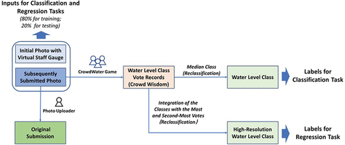
Figure 2. Schematic representation of the dataset construction. The dataset consisted of pairs of photos: the initial photo with virtual staff gauge and a photo at the same spot taken at a later time (see Fig. 1). The citizen scientist who submitted the second photo also submitted a value for the water-level class. The photo pairs were then evaluated in the CrowdWater game, where multiple citizen scientists cast their vote on the water-level class for the second photo. The median of these votes was used as the label for the classification task, while the classes with the highest and second-highest number of votes (see Equations 1(1) $\begin{array}{rl}& C_{\mathrm{h}\mathrm{i}\mathrm{g}\mathrm{h}-\mathrm{r}\mathrm{e}\mathrm{s}\mathrm{o}\mathrm{l}\mathrm{u}\mathrm{t}\mathrm{i}\mathrm{o}\mathrm{n}}=C_{\mathrm{m}\mathrm{a}\mathrm{x}}-\frac{N_{\mathrm{s}\mathrm{e}\mathrm{c}\mathrm{o}\mathrm{n}\mathrm{d}-\mathrm{m}\mathrm{a}\mathrm{x}}}{N_{\mathrm{m}\mathrm{a}\mathrm{x}}+N_{\mathrm{s}\mathrm{e}\mathrm{c}\mathrm{o}\mathrm{n}\mathrm{d}-\mathrm{m}\mathrm{a}\mathrm{x}}}\\ & \mathrm{i}\mathrm{f}{C}_{\mathrm{m}\mathrm{a}\mathrm{x}}\ge C_{\mathrm{s}\mathrm{e}\mathrm{c}\mathrm{o}\mathrm{n}\mathrm{d}-\mathrm{m}\mathrm{a}\mathrm{x}}\end{array}$(1) and 2(2) $\begin{array}{rl}& C_{\mathrm{h}\mathrm{i}\mathrm{g}\mathrm{h}-\mathrm{r}\mathrm{e}\mathrm{s}\mathrm{o}\mathrm{l}\mathrm{u}\mathrm{t}\mathrm{i}\mathrm{o}\mathrm{n}}=C_{\mathrm{m}\mathrm{a}\mathrm{x}}+\frac{N_{\mathrm{s}\mathrm{e}\mathrm{c}\mathrm{o}\mathrm{n}\mathrm{d}-\mathrm{m}\mathrm{a}\mathrm{x}}}{N_{\mathrm{m}\mathrm{a}\mathrm{x}}+N_{\mathrm{s}\mathrm{e}\mathrm{c}\mathrm{o}\mathrm{n}\mathrm{d}-\mathrm{m}\mathrm{a}\mathrm{x}}}\\ & \mathrm{i}\mathrm{f}{C}_{\mathrm{m}\mathrm{a}\mathrm{x}}<C_{\mathrm{s}\mathrm{e}\mathrm{c}\mathrm{o}\mathrm{n}\mathrm{d}-\mathrm{m}\mathrm{a}\mathrm{x}}\end{array}$(2) ) were used as the label for the regression task. For both tasks, the data for the very high and very low water-level classes were merged in the reclassification process to reduce the number of classes for which there were very few observations. The dataset was divided into a training set and a test (or validation) set, with 80% and 20% of all photos for each spot and class, respectively.

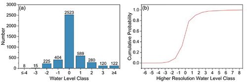
The water level for the photos used in this study varied mainly between class −4 and class 4, with the majority of the photos having a water level in class −1 (9.4%), 0 (58.7%), or 1 (13.7%). Only a few photos from a limited number of spots were taken at a water level lower than class −1 (representing very low water levels) or higher than class 4 (representing very high water levels). To avoid the issue that the number of photos in a certain class was too small compared to that in other classes, photos for the original classes −6 to −4 were merged to form a new class, −4. Similarly, the photos for the original classes ≥ 4 were merged into a new class, +4. This affected 86 of the 4278 (2%) photos (Fig. 3(a)). For the two spots with the most photos, 55 of the 587 and 18 of the 305 photos had to be reclassified. Previous studies have shown that the number of water-level classes does not noticeably influence hydrological model calibration when at least four water-level classes are used (van Meerveld et al. 2017). Therefore, this reclassification is not expected to undermine the value of the crowd-based photos for future hydrological model calibration. For each spot, 80% of the data in each water-level class were randomly selected for the training set, and the remaining 20% were used for validation. The potential impact of the dominance of class 0 (Fig. 3(a)) was eliminated through a weighted loss function (see section 3.4.2).

Figure 3. (a) Number of photos for the different water-level classes after reclassification to nine classes, and (b) the cumulative probability curve for the higher resolution water-level class data (see Equations 1(1) $\begin{array}{rl}& C_{\mathrm{h}\mathrm{i}\mathrm{g}\mathrm{h}-\mathrm{r}\mathrm{e}\mathrm{s}\mathrm{o}\mathrm{l}\mathrm{u}\mathrm{t}\mathrm{i}\mathrm{o}\mathrm{n}}=C_{\mathrm{m}\mathrm{a}\mathrm{x}}-\frac{N_{\mathrm{s}\mathrm{e}\mathrm{c}\mathrm{o}\mathrm{n}\mathrm{d}-\mathrm{m}\mathrm{a}\mathrm{x}}}{N_{\mathrm{m}\mathrm{a}\mathrm{x}}+N_{\mathrm{s}\mathrm{e}\mathrm{c}\mathrm{o}\mathrm{n}\mathrm{d}-\mathrm{m}\mathrm{a}\mathrm{x}}}\\ & \mathrm{i}\mathrm{f}{C}_{\mathrm{m}\mathrm{a}\mathrm{x}}\ge C_{\mathrm{s}\mathrm{e}\mathrm{c}\mathrm{o}\mathrm{n}\mathrm{d}-\mathrm{m}\mathrm{a}\mathrm{x}}\end{array}$(1) and 2(2) $\begin{array}{rl}& C_{\mathrm{h}\mathrm{i}\mathrm{g}\mathrm{h}-\mathrm{r}\mathrm{e}\mathrm{s}\mathrm{o}\mathrm{l}\mathrm{u}\mathrm{t}\mathrm{i}\mathrm{o}\mathrm{n}}=C_{\mathrm{m}\mathrm{a}\mathrm{x}}+\frac{N_{\mathrm{s}\mathrm{e}\mathrm{c}\mathrm{o}\mathrm{n}\mathrm{d}-\mathrm{m}\mathrm{a}\mathrm{x}}}{N_{\mathrm{m}\mathrm{a}\mathrm{x}}+N_{\mathrm{s}\mathrm{e}\mathrm{c}\mathrm{o}\mathrm{n}\mathrm{d}-\mathrm{m}\mathrm{a}\mathrm{x}}}\\ & \mathrm{i}\mathrm{f}{C}_{\mathrm{m}\mathrm{a}\mathrm{x}}<C_{\mathrm{s}\mathrm{e}\mathrm{c}\mathrm{o}\mathrm{n}\mathrm{d}-\mathrm{m}\mathrm{a}\mathrm{x}}\end{array}$(2) ). These frequency curves show the data for all 385 spots combined.

If a similar number of people vote for two adjacent classes, the water level is probably located near the boundary of the two classes. Therefore, in the regression task (see section 3.3), we used the average of the class with the most votes and the class with the second-most votes to derive continuous (rather than discrete) water-level class data for the photo labeling (Fig. 3(b)):

(1) $\begin{array}{rl}& C_{\mathrm{h}\mathrm{i}\mathrm{g}\mathrm{h}-\mathrm{r}\mathrm{e}\mathrm{s}\mathrm{o}\mathrm{l}\mathrm{u}\mathrm{t}\mathrm{i}\mathrm{o}\mathrm{n}}=C_{\mathrm{m}\mathrm{a}\mathrm{x}}-\frac{N_{\mathrm{s}\mathrm{e}\mathrm{c}\mathrm{o}\mathrm{n}\mathrm{d}-\mathrm{m}\mathrm{a}\mathrm{x}}}{N_{\mathrm{m}\mathrm{a}\mathrm{x}}+N_{\mathrm{s}\mathrm{e}\mathrm{c}\mathrm{o}\mathrm{n}\mathrm{d}-\mathrm{m}\mathrm{a}\mathrm{x}}}\\ & \mathrm{i}\mathrm{f}{C}_{\mathrm{m}\mathrm{a}\mathrm{x}}\ge C_{\mathrm{s}\mathrm{e}\mathrm{c}\mathrm{o}\mathrm{n}\mathrm{d}-\mathrm{m}\mathrm{a}\mathrm{x}}\end{array}$(1)

(2) $\begin{array}{rl}& C_{\mathrm{h}\mathrm{i}\mathrm{g}\mathrm{h}-\mathrm{r}\mathrm{e}\mathrm{s}\mathrm{o}\mathrm{l}\mathrm{u}\mathrm{t}\mathrm{i}\mathrm{o}\mathrm{n}}=C_{\mathrm{m}\mathrm{a}\mathrm{x}}+\frac{N_{\mathrm{s}\mathrm{e}\mathrm{c}\mathrm{o}\mathrm{n}\mathrm{d}-\mathrm{m}\mathrm{a}\mathrm{x}}}{N_{\mathrm{m}\mathrm{a}\mathrm{x}}+N_{\mathrm{s}\mathrm{e}\mathrm{c}\mathrm{o}\mathrm{n}\mathrm{d}-\mathrm{m}\mathrm{a}\mathrm{x}}}\\ & \mathrm{i}\mathrm{f}{C}_{\mathrm{m}\mathrm{a}\mathrm{x}}<C_{\mathrm{s}\mathrm{e}\mathrm{c}\mathrm{o}\mathrm{n}\mathrm{d}-\mathrm{m}\mathrm{a}\mathrm{x}}\end{array}$(2)

where $C_{\mathrm{h}\mathrm{i}\mathrm{g}\mathrm{h}-\mathrm{r}\mathrm{e}\mathrm{s}\mathrm{o}\mathrm{l}\mathrm{u}\mathrm{t}\mathrm{i}\mathrm{o}\mathrm{n}}$ represents the continuous (i.e. higher-resolution) water-level class, $C_{\mathrm{m}\mathrm{a}\mathrm{x}}$ and $C_{\mathrm{s}\mathrm{e}\mathrm{c}\mathrm{o}\mathrm{n}\mathrm{d}-\mathrm{m}\mathrm{a}\mathrm{x}}$ denote the class with the highest and the second-highest number of votes, respectively. $N_{\mathrm{m}\mathrm{a}\mathrm{x}}$ and $N_{\mathrm{s}\mathrm{e}\mathrm{c}\mathrm{o}\mathrm{n}\mathrm{d}-\mathrm{m}\mathrm{a}\mathrm{x}}$ are the number of votes for these two classes. Only for the photos for which citizen scientists in the CrowdWater game chose more than one class was a new synthetic class derived. The mean value of the standard deviation of the votes for each photo was 0.46 classes. The maximum standard deviation was 3.5 classes.

3 Methods

3.1 General approach

The idea of the virtual staff gauge used in the CrowdWater app is to enable the monitoring of water-level class changes by comparing observations of the current water level to the water level at a previous time (Fig. 1). The objective of this study is to test whether it is possible to automatically estimate the water level for a newly uploaded photo by comparing it with the initial photo that includes the virtual staff gauge. The approach is schematically shown in Fig. 4. The model was fed with two photos as inputs: the initial photo with the image of the virtual staff gauge added to it and the photo that was taken at the same spot at a later time (Figs. 4 and 5). The same feature extraction module of the deep learning model was applied to both photos. The extracted feature vectors were then concatenated and passed to the classifier module for water-level class estimation. Based on learning from such a comparative analysis (Le-Khac et al. 2020), the method enables the extracted feature of sample pairs to be implicitly measured and, in this case, to detect the variation in water level from the two photos.

Figure 4. Schematic illustration of the steps used in model training and evaluation in this study. In the training stage, the model used photo pairs from the training dataset (80% of all photo pairs) as input, predicted the water-level class, calculated the loss function based on the true values, and updated the model parameters using different training strategies (semi-trained or fully-trained). In the evaluation stage, the trained model predicted the water-level class for the photo pairs from the test dataset (20% of all photo pairs), and the results were compared to the true water-level class (i.e. water-level class from the game) to calculate the evaluation metrics. These metrics were also calculated for the water-level class provided by the citizen scientist who uploaded the photo.

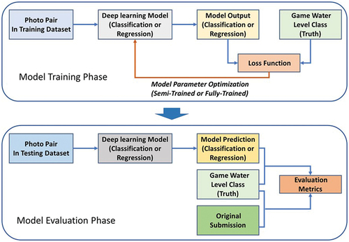
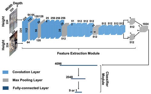
Figure 5. Set-up of the model used in this study. The model is composed of two parts: the feature extraction module and classifier module. The initial photo with the virtual staff gauge and the photo taken at the same spot at a later time go through the feature extraction module separately. The extracted features are subsequently concatenated and processed in the second module to accomplish the classification or regression task. The feature extraction module follows the VGG 19 model and is constructed by stacking multiple convolution layers and max pooling layers. The classifier module mainly depends on a series of fully-connected layers. The ReLU function was used after each convolution layer. The height, width and channel number of the input images and vectors in each step are indicated in the figure.

The automatic comparison of the water level in crowd-based photos to determine the (changes in) water level can be treated as either a classification or a regression task. In the regression task, the model used continuous rather than discrete data. By comparing the performance for the two tasks, the potential of the model to derive a time series with higher resolution water-level class data can be explored. For the classification task, we compared two training strategies (fully-trained and semi-trained), and explored the effect of the large number of photos for which the water level was in class 0. Finally, we determined the effect of the training dataset size for both tasks.

3.2 Ranking photos with convolutional neural networks

We adopted convolutional neural networks (CNNs) (Krizhevsky et al. 2012) as the backbone of our model for ranking the time series of crowd-based photos of streams. CNNs are based on the neural network architecture (Aloysius and Geetha 2017), consisting of an input layer, several intermediate hidden layers, and an output layer. The hidden layers of CNNs can be classified into three types: (I) convolution layers, (II) pooling layers, and (III) fully-connected layers. Convolution layers are mainly used for feature extraction, while pooling and fully-connected layers are used for dimension reduction and subsequent activation.

As shown in Fig. 6, in the convolution layer, a kernel is applied to a small region of the image and element-wise multiplication is conducted between the kernel and the corresponding image region. The resulting values from this multiplication are summed. The filter then shifts in stride increments to the next region of the image, repeating the process. Ultimately, the aggregated outcomes, commonly called feature maps, are arranged into a new output matrix. The movement of the window in the pooling layer is similar to that in the convolution layer, but instead of executing element-wise multiplication, the maximum or average value within the window is extracted. The fully-connected layer connects every neuron from the previous layer to every neuron in the current layer, forming a fully-connected network structure. Unlike convolution and pooling layers, the fully-connected layer does not consider spatial relationships or local patterns in the input data. Instead, it treats the input as a flat vector.

Figure 6. Schematic representation of the convolution and max-pooling operation in the CNN model.

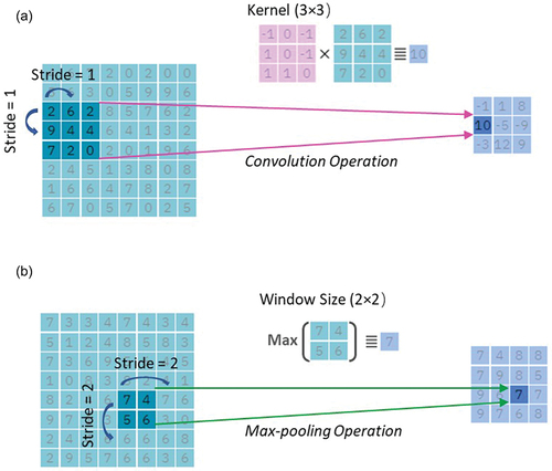
The set-up of convolution and pooling layers of the CNN used in this study were identical to those of the VGG19 batch normalization model (Simonyan and Zisserman 2015). VGG19 is a model widely employed for image data that uses deep visual representations in computer vision. The feature extraction module of VGG19 is composed of a stack of convolution layers. The filters used in these layers have a very small receptive field: 3 × 3. In other words, the kernel in the convolution layers was a 3 × 3 matrix, where 3 × 3 is the smallest size needed to capture the notion of left/right, up/down and centre. The convolution stride was fixed to 1 pixel. Spatial pooling was carried out by five max-pooling layers, which follow some of the convolution layers. Max-pooling was performed over a 2 × 2 pixel window, with stride 2. Finally, three consecutive fully-connected layers were used to realize the successive dimension reduction of the high-dimensional features extracted from the previous convolution and pooling layers. For the classification task, the channel number in the last layer was set to the number of the target class. For the regression task, it was set to 1. The channel number in other layers was based on experience and feature dimension.

All hidden layers in the VGG19 model were equipped with a linear rectification function (ReLU) for non-linearity to enhance the fitting ability (Krizhevsky et al. 2012). A batch normalization layer was inserted after each convolution layer and each fully-connected layer to accelerate the training and make the training performance less dependent on the initial model parameter values (Thakkar et al. 2018). Batch normalization can be implemented during training by calculating the mean and standard deviation of each input variable for a layer per mini-batch, which is a batch of a fixed number of training examples (Nielsen 2015). These statistics were used for standardization.

Additionally, dropout regularization was added between the network layers during model training. This means that a certain number of randomly selected units (hidden and visible) in a neural network are left out (Goodfellow et al. 2016). This operation can help avoid overfitting as it has been shown that the pre-trained network (VGG19) parameters can be fine-tuned for different image classification tasks by transfer learning (Shaha and Pawar 2018). Therefore, in our study, we transferred the parameters in the convolution and pooling layers of the VGG19 batch normalization model pre-trained on the ImageNet dataset (Deng et al. 2009). All subsequent training was initialized from the transferred parameters. The inputs of the feature extraction module were two 224 × 224 RGB photos, and the output was a 7 × 7 × 512 dimension feature vector (Figs. 5 and 6).

3.3 Classification and regression tasks

The automatic comparison of the water level in crowd-based photos to determine the changes in water level can be treated as a classification or regression task. If people vote for two adjacent classes in the CrowdWater game, it may indicate that the water level is located near the boundary of the two classes. We therefore used the continuous water-level class data (as per Equations 1(1) $\begin{array}{rl}& C_{\mathrm{h}\mathrm{i}\mathrm{g}\mathrm{h}-\mathrm{r}\mathrm{e}\mathrm{s}\mathrm{o}\mathrm{l}\mathrm{u}\mathrm{t}\mathrm{i}\mathrm{o}\mathrm{n}}=C_{\mathrm{m}\mathrm{a}\mathrm{x}}-\frac{N_{\mathrm{s}\mathrm{e}\mathrm{c}\mathrm{o}\mathrm{n}\mathrm{d}-\mathrm{m}\mathrm{a}\mathrm{x}}}{N_{\mathrm{m}\mathrm{a}\mathrm{x}}+N_{\mathrm{s}\mathrm{e}\mathrm{c}\mathrm{o}\mathrm{n}\mathrm{d}-\mathrm{m}\mathrm{a}\mathrm{x}}}\\ & \mathrm{i}\mathrm{f}{C}_{\mathrm{m}\mathrm{a}\mathrm{x}}\ge C_{\mathrm{s}\mathrm{e}\mathrm{c}\mathrm{o}\mathrm{n}\mathrm{d}-\mathrm{m}\mathrm{a}\mathrm{x}}\end{array}$(1) and 2(2) $\begin{array}{rl}& C_{\mathrm{h}\mathrm{i}\mathrm{g}\mathrm{h}-\mathrm{r}\mathrm{e}\mathrm{s}\mathrm{o}\mathrm{l}\mathrm{u}\mathrm{t}\mathrm{i}\mathrm{o}\mathrm{n}}=C_{\mathrm{m}\mathrm{a}\mathrm{x}}+\frac{N_{\mathrm{s}\mathrm{e}\mathrm{c}\mathrm{o}\mathrm{n}\mathrm{d}-\mathrm{m}\mathrm{a}\mathrm{x}}}{N_{\mathrm{m}\mathrm{a}\mathrm{x}}+N_{\mathrm{s}\mathrm{e}\mathrm{c}\mathrm{o}\mathrm{n}\mathrm{d}-\mathrm{m}\mathrm{a}\mathrm{x}}}\\ & \mathrm{i}\mathrm{f}{C}_{\mathrm{m}\mathrm{a}\mathrm{x}}<C_{\mathrm{s}\mathrm{e}\mathrm{c}\mathrm{o}\mathrm{n}\mathrm{d}-\mathrm{m}\mathrm{a}\mathrm{x}}\end{array}$(2) ) for the regression task and the median water-level class data for the classification task (Figs. 2 and 4). However, the classification model provides the probability that the image belongs to different classes rather than a single class estimate, which, like the regression model, can potentially assist in obtaining finer class resolution data.

The CNN for the classification and regression tasks is similar to the convolution layers and pooling layers introduced in section 3.2 (Figs. 5 and 6). The extracted feature vector from the two parts is fed into the fully-connected layers for subsequent processing. For the classification, the water-level class was determined according to the output probability of a photo that belongs to a specific class and then used for ranking the photos. Thus, the output is the vector with the same number of dimensions as the target classes. For the regression, the scalar value of the output for each photo (a one-dimensional variable) directly represents the corresponding water-level class. Correspondingly, the hyper-parameter of the classifier module varied with the task type. The first two fully-connected layers had 4096 and 2048 channels. For the last fully-connected layer, the channel number was set to 9 in the classification task and 1 for the regression task. The subsequent model application comprised model training and evaluation phases, illustrated in Fig. 4.

3.4 Training

3.4.1 Training strategies

The photo pairs used for training were put into the model in batches, with a batch size of 16. L2 regularization was used to overcome overfitting in training datasets (Cortes et al. 2004). We compared two training strategies with different parameter optimization strategies for the classification task: fully-trained and semi-trained. We did not repeat this for the regression task because the main parameters to be updated are similar for the classification and regression tasks. Therefore, the more optimal training strategy for the regression task was also used in classification.

For the fully-trained strategy, the entire neural network was fine-tuned. The initial weights of the convolution and pooling layers were equal to the weights of the feature extraction module transferred from the VGG19 batch normalization model. In contrast, the weights of the three fully-connected layers were initialized randomly. For the semi-trained strategy, only the weights in the classifier module of the fully-connected layers were optimized. The parameters in the feature extraction module were the same as those of the source network layers.

For the training, the number of training epochs was set to 200. For the first 100 epochs, the learning rate was set to 0.0001, and from the 101^st epoch to the 200^th epoch, the learning rate decreased by 50% to fine-tune the model parameters. The model that achieved the lowest loss value in the 200 epochs for the training datasets was selected as the optimal model for subsequent evaluation and analysis.

3.4.2 Loss function

The cross-entropy function ($L_{CE}$) was selected as the loss function for model training in the classification task. The cross-entropy loss measures the degree to which the predicted probabilities of different classes diverge from the actual label and is defined as:

(3) $L_{CE}=-\sum _i^K{s}_{i}log\left(s_i\right)$(3)

where K equals the number of the target classes and $s_i$ refers to the values corresponding to different dimensions of the input vector.

During the training, specific weights were assigned to photos to cope with the imbalance in the number of photos in the different classes (Fig. 3). The assigned weight for a specific class was inversely proportional to the total number of photos for that class:

(4) ${\mathrm{\ell }}_{\mathrm{k}}^{\prime }=\frac{N_{total}}{N_k}{\mathrm{\ell }}_{\mathrm{k}}$(4)

where ${\mathrm{\ell }}_{\mathrm{k}}^{\prime }$ represents the transformed loss, ${\mathrm{\ell }}_{\mathrm{k}}$ denotes the originally calculated loss, and $N_k$ and $N_{total}$ represent the number of photos in class k and the total number of photos, respectively.

For the regression task, the model was trained on both the regression sub-task and the ranking sub-task by defining the total loss function as in Chaudhary et al. (2020):

(5) ${\mathrm{\ell }}_{\mathrm{t}\mathrm{o}\mathrm{t}\mathrm{a}\mathrm{l}}={\mathrm{\ell }}_{reg}+\alpha {\mathrm{\ell }}_{rank}$(5)

where ${\mathrm{\ell }}_{reg}$ represents the regression loss, ${\mathrm{\ell }}_{rank}$ denotes the ranking loss, and $\alpha$ is the weighting parameter to balance the contributions of the two terms. The mean squared error (MSE) was used to quantify ${\mathrm{\ell }}_{reg}$:

(6) ${\mathrm{\ell }}_{reg}=(y-y_{gt}{)}^2$(6)

where $y$ and $y_{gt}$ represent the estimation and the ground truth of the water-level class. The ranking loss was computed as:

(7) ${\mathrm{\ell }}_{rank}=max(0,-\left(y_1-y_2\right)\cdot \left(y_{gt1}-y_{gt2}\right))$(7)

where $y_1$ and $y_2$ represent the network output of two pairs of photos and $y_{gt1}$ and $y_{gt2}$ are the annotated water-level class for the two photos that have to be compared (i.e. considered to be the truth). If the ranking relation between $y_1$ and $y_2$ is consistent with that of $y_{gt1}$ and $y_{gt2}$, the loss decreases, and conversely, if the ranking relation is inconsistent, the loss increases.

By integrating the two loss functions, it is expected that the model not only fits the ground truth but also considers the ranking relation between the photos. In this study, the weighting parameter, $\alpha$, was set to 10 to strengthen the ability of the model to rank the water levels but not to undermine the model fit.

3.5 Model evaluation

The model performance was evaluated with three metrics: accuracy (A), root mean square error (R) and Spearman’s rank correlation coefficient (r_s). A higher value of A or r_s, or a lower value of R, indicates an overall better model performance. In other words, A and r_s = 1 and R = 0 represent a perfect model performance. R and r_s were used for the evaluation of the classification and regression tasks; accuracy was only used for the classification tasks.

Accuracy A describes the percentage of photos that are accurately classified. It is a frequently used indicator to evaluate the classification of a certain class:

(8) $A=\frac{N_k}{N_{total}}$(8)

where $N_{total}$ and $N_k$ indicate the total number of photos and the correctly predicted number of photos in class $k$, respectively.

The root mean square error (R) is commonly used to demonstrate how concentrated the data is around the line of best fit. In this study, it was used to quantify the difference (i.e. error) between the water-level class estimated by the model and the water-level class determined by the citizen scientists (i.e. the “truth”):

(9) $R=\sqrt{\frac{{\sum }_{t=1}^n{({\hat{y}}_t-y_t)}^2}{n}}$(9)

where ${\hat{y}}_t$ and $y_t$ are the estimated (model) and true (citizen derived) water-level class, respectively, and $n$ represents the number of photos that are evaluated for that spot.

The Spearman rank correlation coefficient (r_s) was used to evaluate the model’s ability to rank the water level, and, more specifically, to describe the degree of association between the estimated and the continuous water-level class.

We also compared the performance of the deep learning model with the water-level class that was reported by the citizen scientist who submitted the photo (referred to as the “original submission” through the remainder of the text). Remember that we assumed the median vote from the game represented the truth and the water-level class reported by the citizen scientist who submitted the photo could be wrong. Admittedly, it is also still possible that the median vote from the game is wrong.

All the evaluations were done for the testing dataset. Only the spots with observations in at least two different classes in the testing dataset (112 spots) can be evaluated with r_s for the classification tasks. For subsequent comparisons between the two tasks, r_s was only calculated for these 112 spots for the regression task.

3.6 Effect of training dataset

It is important to determine the appropriate amount of training data for the model, as too little training data leads to under-fitting but more data also means a larger classification effort. The influence of the amount of training data on model performance was analysed by training the model for each spot with a different number of photos ($2^{n-1}-2^n$, n = 1, 2, 3, 4, 5, 6). To determine the potential impact of the dominance of observations of water-level class 0 on model performance, the Spearman rank correlation coefficient was also calculated excluding all the class 0 data for the semi-trained model and original submissions by the citizen scientists. This was done for the 56 spots with observations in at least two non-zero classes (1468 photos in total).

4 Results

4.1 Classification task

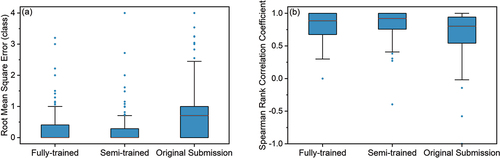
The performance for the fully-trained and semi-trained models was similar: the root mean square error (R) and accuracy (A) were 0.69 and 0.70, respectively, for the fully-trained model, and 0.70 and 0.68 for the semi-trained model (Fig. 7). The Spearman rank correlation coefficient was higher than 0.75 for most of the spots (for 77% and 70% of all 112 spots for which the water-level class varied by more than two classes for the semi-trained model and fully-trained models, respectively).

Figure 7. Box plots of (a) the root mean square error R and (b) the Spearman rank correlation coefficient r_s for of the fully-trained and semi-trained models for the classification task and for the water-level class estimated by the citizen scientist who submitted the photo. R was calculated for all 385 spots, while r_s could only be evaluated for the 112 spots for which the water-level class varied over at least two classes. The median vote for a photo in the CrowdWater game was assumed to be the truth. The upper and lower boundary of the box represent the upper (0.75) and lower (0.25) quartiles, the solid line is the median, the whiskers extend to 1.5 times the interquartile range, and the dots are outliers.

The values of R and A for the different water-level classes indicated that the estimate of the deep learning models was better (i.e. closer to the median water-level class from the game) than the water-level class estimated by the citizen who submitted the photo for water-level classes −2 to 0 (Table 1). The value A of these three water-level classes was higher than 0.65 and the value of R was less than one class. For water-level class 4, the estimate of the citizen scientist better matched the game-derived water-level class than the model derived water-level class. The value A of the estimate by the citizen scientist who submitted the photo reached 0.88 and the value of R was only 0.35 classes, while A and R were 0.32 and 1.64 for the fully-trained model and 0.68 and 1.56 for the semi-trained models. Moreover, the model results were not as good for class 1 as for class −1 (Table 1).

Table 1. The accuracy (A [-]) and root mean square error (R [classes]) for the testing dataset for images with different water-level classes.

Water-level class	Number of images n	Fully-trained model		Semi-trained model		Original submission
		A	R	A	R	A	R
−4	2	1.00	0.00	1.00	0.00	1.00	0.00
−3	4	1.00	0.00	0.25	0.87	0.25	0.87
−2	46	0.76	0.55	0.80	0.51	0.50	1.22
−1	82	0.70	0.76	0.65	0.65	0.45	1.14
0	506	0.76	0.59	0.79	0.55	0.59	0.99
1	119	0.54	0.86	0.52	0.85	0.60	0.76
2	57	0.56	0.89	0.51	0.97	0.44	0.96
3	25	0.44	1.11	0.24	1.36	0.52	0.69
4	25	0.32	1.64	0.68	1.56	0.88	0.35

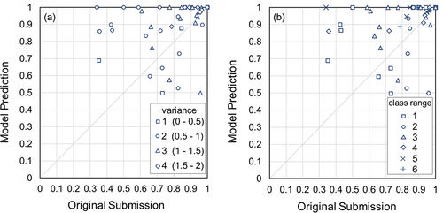
When excluding all the class 0 data, the Spearman rank correlation coefficient was still higher for the semi-trained model prediction than for the original readings by the citizen scientists who submitted the photo for 47 of the 56 spots with observations in at least two non-zero classes (Fig. 8). For 48 of these 56 spots, the Spearman rank correlation coefficient was higher than 0.75.

Figure 8. Relation between the Spearman rank correlation coefficient r_s for the water-level class identified by the citizen scientists who submitted the photo (x-axis) and the semi-trained model (y-axis) for the 56 spots for which observations were available for at least two different water-level classes after excluding the class 0 observations. The median of the vote for an image in the CrowdWater game was used as the truth. The shapes of the spots in (a) indicate the variance, and in (b) they show the range of water-level class observations. The result for the one spot for which the r_s is negative is not shown.

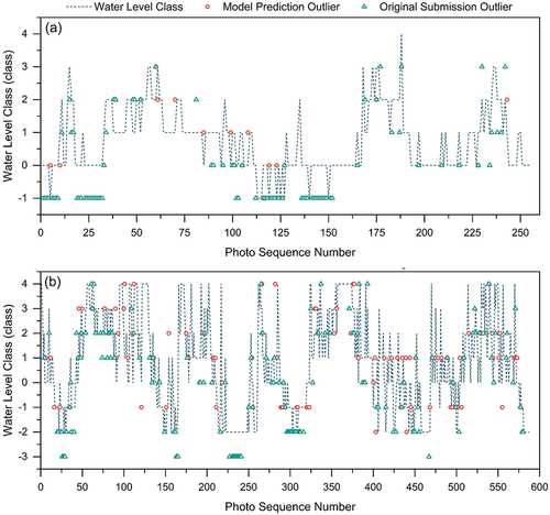
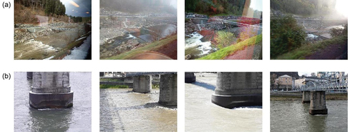
Data from two spots were used to further analyse the performance of the semi-trained model. For Location 1, there was no photo for which the model error was more than two classes (Fig. 9(a)) due to the relatively steady background and shoot distance for each photo (n = 255). This was not the case for Location 2 for which there were the most photos (n = 587). There was a systematic error in the original submissions, but the model error was more random (Fig. 9(b)). In Fig. 1, six wrongly classified photos for Location 2 (i.e. an error of more than two classes) are shown to illustrate the main factors causing the model errors. When there were obstacles in front of the camera, such as branches (Fig. 1(b) and (d)) that did not exist in the original reference photo, when the reference object was covered with snow (Fig. 1(c)), or when there was too much vegetation (Fig. 1(f)), this interfered with the classification and the model was confused. When the lens was too close or too far, the visual angle and distance changed, which influenced the classification as well. Figure 1(c) is an example where the wrong classification was caused by snow and the distance between the camera and the reference object (shorter than in the original photo). Other reasons for errors included the effect of light and shadow, as well as the movement of the lens (Fig. 1(e)).

Figure 9. The water-level class based on the median vote from the game (i.e. ground truth; blue line) for all the analysed photos, and the corresponding semi-trained model predictions (red dot) and original submissions (green triangle) where they do not match the ground truth for two example spots (Location 1 (a) and 2 (b)). For visualization, only the results for the wrongly classified photos are shown; those that were predicted correctly by the model or submitted correctly by the citizen scientists are not shown (and would plot on the blue line). The photo numbers are in chronological order, but the time interval between adjacent photos differs.

The difference between the original submission and model result was related to the water-level class range (i.e. the difference between the maximum and minimum water-level class observed) for a specific spot, as well as the variance in the observed water-level class data (Fig. 8). The superiority of the model prediction to the original observations tended to be more significant (far from the dotted line in Fig. 8, upward) when the water level varied over more than three classes. Especially when the size of the virtual staff was not appropriate (generally, too large), humans tended to misclassify the photos of two adjacent water-level classes. At the same time, the deep learning model could better distinguish the variance. However, the model might provide less accurate water-level class prediction for some spots where the water level varied only within two classes.

Despite the overall good performance of the model, there were also some spots with a large model prediction uncertainty and for which the Spearman rank correlations were negative. The uncertainty in the water-level class estimates for these spots was related to the quality of the photos. For one spot, the photos were taken from a moving train and were apparently not clear enough for water-level classification (Fig. 10(a)). For another spot the large difference between the model prediction and water-level classes estimated by the citizen scientists who played the CrowdWater game appears to be related to the drastic variation in the sight distance and visual angle of the photos (Fig. 10(b)).

Figure 10. Example photos for two spots for which the model performance was not satisfactory: photos taken (a) from a moving train resulting in a negative Spearman rank correlation coefficient r_s for both the model and the original observation (photos from: https://www.spotteron.com/crowdwater/spots/40237), and (b) for a spot where the Spearman rank correlation is lower for the model than for the original submission because the sight distance and visual angle differ considerably from one photo to another (photos from: https://www.spotteron.com/crowdwater/spots/22036).

4.2 Regression task

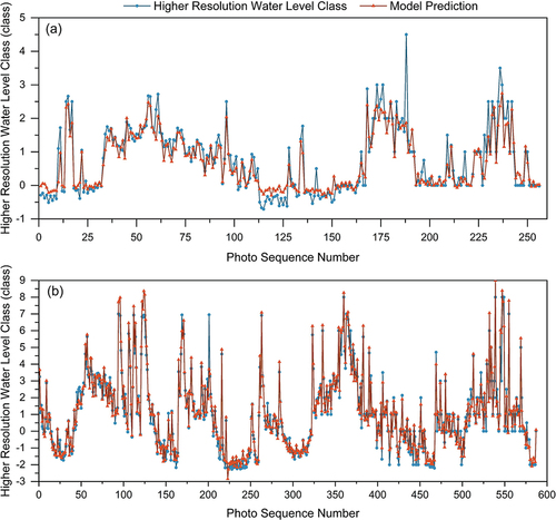
In the regression task, we evaluated the model performance when it was trained with continuous water-level class data using the semi-trained strategy. The median R was 0.13 for the regression task (Fig. 11(a)). Although the median R was smaller than for the classification task (0.2 classes), this difference was not significant (p = .75 for the Mann-Whitney U test). The median Spearman rank correlation coefficient was 0.85 (Fig. 11(b)). This was also not significantly higher than for the classification task (0.73; p = .056). Both metrics indicated that the model appropriately fit the high-resolution water-level class data, as also indicated by the time series for two spots with many photos (Fig. 12).

Figure 11. Box plots of (a) the root mean square error R and (b) the Spearman rank correlation coefficient r_s of the water-level class time series for the classification and regression models (semi-trained). R was calculated for all 385 spots, and r_s only for the 112 spots for which the water-level class varied over at least two classes. For the classification task, the photos were compared with the median vote from the CrowdWater game. For the regression task, the classes with the most and the second most votes in the game were used to derive higher resolution class data for the photos (see Fig. 2 for a schematic representation). Note that the result for the one outlier for the classification model with a root mean square error of 4.8 classes is not shown.

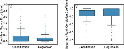
Figure 12. The water-level class data (Equations 1(1) $\begin{array}{rl}& C_{\mathrm{h}\mathrm{i}\mathrm{g}\mathrm{h}-\mathrm{r}\mathrm{e}\mathrm{s}\mathrm{o}\mathrm{l}\mathrm{u}\mathrm{t}\mathrm{i}\mathrm{o}\mathrm{n}}=C_{\mathrm{m}\mathrm{a}\mathrm{x}}-\frac{N_{\mathrm{s}\mathrm{e}\mathrm{c}\mathrm{o}\mathrm{n}\mathrm{d}-\mathrm{m}\mathrm{a}\mathrm{x}}}{N_{\mathrm{m}\mathrm{a}\mathrm{x}}+N_{\mathrm{s}\mathrm{e}\mathrm{c}\mathrm{o}\mathrm{n}\mathrm{d}-\mathrm{m}\mathrm{a}\mathrm{x}}}\\ & \mathrm{i}\mathrm{f}{C}_{\mathrm{m}\mathrm{a}\mathrm{x}}\ge C_{\mathrm{s}\mathrm{e}\mathrm{c}\mathrm{o}\mathrm{n}\mathrm{d}-\mathrm{m}\mathrm{a}\mathrm{x}}\end{array}$(1) and 2(2) $\begin{array}{rl}& C_{\mathrm{h}\mathrm{i}\mathrm{g}\mathrm{h}-\mathrm{r}\mathrm{e}\mathrm{s}\mathrm{o}\mathrm{l}\mathrm{u}\mathrm{t}\mathrm{i}\mathrm{o}\mathrm{n}}=C_{\mathrm{m}\mathrm{a}\mathrm{x}}+\frac{N_{\mathrm{s}\mathrm{e}\mathrm{c}\mathrm{o}\mathrm{n}\mathrm{d}-\mathrm{m}\mathrm{a}\mathrm{x}}}{N_{\mathrm{m}\mathrm{a}\mathrm{x}}+N_{\mathrm{s}\mathrm{e}\mathrm{c}\mathrm{o}\mathrm{n}\mathrm{d}-\mathrm{m}\mathrm{a}\mathrm{x}}}\\ & \mathrm{i}\mathrm{f}{C}_{\mathrm{m}\mathrm{a}\mathrm{x}}<C_{\mathrm{s}\mathrm{e}\mathrm{c}\mathrm{o}\mathrm{n}\mathrm{d}-\mathrm{m}\mathrm{a}\mathrm{x}}\end{array}$(2) ) and regression model estimates for two spots (Location 1 and 2). The photo numbers are in chronological order, but the time interval between adjacent photos differs.

The results of the regression model used to obtain higher resolution data were better than those of the classification model. Although the correlation between the class with the highest probability based on the classification model and the most votes was as high as 0.89, it was only 0.48 between the class with the second highest probability and the second most votes in the game. This meant that the two were weakly correlated. Consequently, the regression model was considered a more appropriate choice for deriving higher-resolution results than the classification model.

4.3 Influence of the number of training photos on model performance

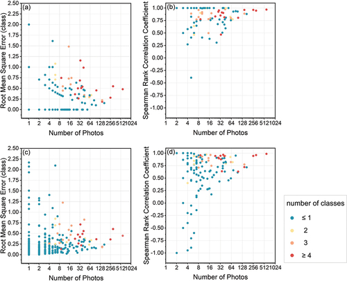
According to Fig. 13(a)–(d), the model’s predictive performance for a particular spot was positively correlated with the number of photos contributed by the citizen scientists for that spot. For most spots for which more than 64 photos were used for model training for the classification task, R was less than 0.5 classes and the Spearman rank correlation coefficient was higher than 0.75 (Fig. 13(a) and (b)). When the sample size was less than 64, the model performance was highly variable. This was also the case for the regression task (Fig. 13(c) and (d)). However, R was larger than 0.5 classes for one spot (spot 42809) with 305 photos for both the classification and regression tasks. This spot was located under a bridge and shows a row of pillars. The angles and scaling factors for the photos for this spot varied greatly and appear to have challenged the model.

Figure 13. Influence of the number of training photos on model performance in terms of root mean square error R (a and c) and Spearman rank correlation coefficient r_s (b and d) for the classification task (a, b) and regression task (c, d). Each dot represents one spot and is coloured by the number of classes over which the water level varied in the photos for that spot.

5 Discussion

5.1 Performance of the models

Computer vision techniques can be used to determine the relative position of the water level in time-lapse camera images or videos (Chaudhary et al. 2019). However, photos taken by citizen scientists differ from time-lapse camera images in terms of the angle, distance, light conditions, etc. This makes it more difficult to determine the water level from these photos automatically. The deep learning model proposed in this study provides a new way to estimate the water-level class from crowd-based photos. Unlike the traditional method of extracting water-level information from photos based on reference object segmentation or water segmentation, the applied method enables the extracted feature of photo pairs to be implicitly measured based on a comparative representation learning framework (Le-Khac et al. 2020). The results of this study show that the deep learning model can detect the variation in water level from photos taken at different times at the same location, even if these photos differ in angle, distance to the object, camera type, etc. The deep learning models are expected to have even better accuracy when applied to fixed-angle photos, such as those from time-lapse cameras.

Both the fully-trained model and the semi-trained model captured the water level variations well and can thus be used to check and improve the water-level class observations that citizen scientists submit. The training process of the deep learning model is equivalent to searching the parameter space to fit the training data based on a loss function. Thus, selecting the suitable training strategy is a trade-off between the model parameters and the available training data. For the semi-trained strategy, the parameters of the feature extraction module were fixed. This narrows the range for the parameter search compared to the fully-trained strategy. When the amount of training data is only on the order of 1000, as in our study, reducing the number of parameters for optimization enables the model to fit the training data more easily. Therefore, we conclude that the semi-trained strategy is likely the more effective way for training the model to determine the water-level class for citizen science data.

The method provided acceptable results in terms of ranking the water level, for both the classification task and the regression task. Overall, the regression task performed slightly better than the classification task. However, the probability of the photo belonging to different water-level classes estimated by the classification model could not be used to derive higher resolution water-level classes. Formalizing the water level ranking into a regression task by directly training the model with the continuous water-level class data derived from CrowdWater game (Equations 1 and(1) $\begin{array}{rl}& C_{\mathrm{h}\mathrm{i}\mathrm{g}\mathrm{h}-\mathrm{r}\mathrm{e}\mathrm{s}\mathrm{o}\mathrm{l}\mathrm{u}\mathrm{t}\mathrm{i}\mathrm{o}\mathrm{n}}=C_{\mathrm{m}\mathrm{a}\mathrm{x}}-\frac{N_{\mathrm{s}\mathrm{e}\mathrm{c}\mathrm{o}\mathrm{n}\mathrm{d}-\mathrm{m}\mathrm{a}\mathrm{x}}}{N_{\mathrm{m}\mathrm{a}\mathrm{x}}+N_{\mathrm{s}\mathrm{e}\mathrm{c}\mathrm{o}\mathrm{n}\mathrm{d}-\mathrm{m}\mathrm{a}\mathrm{x}}}\\ & \mathrm{i}\mathrm{f}{C}_{\mathrm{m}\mathrm{a}\mathrm{x}}\ge C_{\mathrm{s}\mathrm{e}\mathrm{c}\mathrm{o}\mathrm{n}\mathrm{d}-\mathrm{m}\mathrm{a}\mathrm{x}}\end{array}$(1) 2(2) $\begin{array}{rl}& C_{\mathrm{h}\mathrm{i}\mathrm{g}\mathrm{h}-\mathrm{r}\mathrm{e}\mathrm{s}\mathrm{o}\mathrm{l}\mathrm{u}\mathrm{t}\mathrm{i}\mathrm{o}\mathrm{n}}=C_{\mathrm{m}\mathrm{a}\mathrm{x}}+\frac{N_{\mathrm{s}\mathrm{e}\mathrm{c}\mathrm{o}\mathrm{n}\mathrm{d}-\mathrm{m}\mathrm{a}\mathrm{x}}}{N_{\mathrm{m}\mathrm{a}\mathrm{x}}+N_{\mathrm{s}\mathrm{e}\mathrm{c}\mathrm{o}\mathrm{n}\mathrm{d}-\mathrm{m}\mathrm{a}\mathrm{x}}}\\ & \mathrm{i}\mathrm{f}{C}_{\mathrm{m}\mathrm{a}\mathrm{x}}<C_{\mathrm{s}\mathrm{e}\mathrm{c}\mathrm{o}\mathrm{n}\mathrm{d}-\mathrm{m}\mathrm{a}\mathrm{x}}\end{array}$(2) ) is a better way to estimate the water-level class from the photos with a higher resolution. Thus, the superiority of the regression model over the classification model in exploiting the distribution of votes from the CrowdWater game (i.e. higher resolution data) indicates a higher value for the regression model when the data are to be used for hydrological model calibration or other analyses. In addition, the regression model is trained based on the combined assessment of all the players of the CrowdWater game.

The models’ capabilities in classifying high water levels can be improved. The deep learning model estimates the water-level class by inferring the relative position between the reference object in the photos and the water surface. When the water level decreases, the original reference object remains completely visible, but if the water level rises, the water covers part of the reference object. This probably confuses the model when quantifying the relative distance between the water surface and the reference object. This inference is supported by the difference in model performance for the two water-level classes directly below and above the water level of the reference photo (classes −1 and 1), for which a relatively large number of photos were available. However, more quantitative experiments are needed to confirm this. The poorer performance of the model at high water levels calls for more photos at high water levels to train the model. Perhaps this will reduce the gap between the model and human assessments of the high water levels. Still, for now, it is better to implement the data-driven model as a supportive tool (e.g. for data quality control) rather than as an alternative to crowd-based observations to obtain reliable water-level class estimates from the time series of crowd-based photos.

The model performance was also weaker when photos were taken from very different angles or distances or when they were blurry. This is consistent with previous findings that image resolution, light, perspective and lens distortion all add to the uncertainty of image-based water level measurements (Gilmore et al. 2013, Herzog et al. 2022). It also suggests that it is useful to ask citizen scientists to upload photos that are as similar to the reference photo as possible, to train the model. However, the differences in angles, distances, and blurriness between the initial photo and subsequent photos were only qualitatively characterized in this study. Future studies can attempt to apply the data-driven spatial analysis method, such as the deep depth prediction model (Laina et al. 2016), to the crowd-based photos. The differences in shooting conditions across photos can potentially be quantitatively characterized by these methods and used to guide the photo submission of citizen scientists more explicitly and in real time.

The photos were labelled based on the aggregated voting results from the CrowdWater game. While the integrated outcome of the votes is more reliable than the initial submission provided by the person who uploaded the photo (Strobl et al. 2019), it may (like any other data) still contain errors. To ensure a more objective assessment of the model’s performance, future studies could select a set of spots, install water level loggers and collect quantitative water level data for model training and validation. The use of continuous water level data can potentially improve the accuracy of the model beyond the current version, which relies on the wisdom of the crowd. However, there is a good agreement between the observed water level and the water-level class that is reported by the person who submits the data (Etter et al. 2020b, Strobl et al. 2020) and the CrowdWater game improves the quality of the data even further (Strobl et al. 2019). Therefore, we expect that this will not lead to a very large improvement in model performance.

Although we assumed that the deep learning model estimates the water-level class by inferring the relative positional relationship between the reference object in the photo and the water surface, this has not been validated yet. Thus, the internal mechanisms of the deep learning model, such as what features in the photo are informative for water-level classification, remain to be analysed in future studies. This is important for model structure modification and improving the model’s performance. Novel diagnosis methods for deep learning models, including discriminative localization (Rajaraman et al. 2018) and embedding attention mechanism (Karpov et al. 2020), can be useful for this.

5.2 Human–computer interaction for data quality control in citizen science projects

A good dataset is crucial for training deep learning models. However, creating manually annotated images is time-consuming. Many studies have tried to exploit the power of the public to increase the efficiency of data annotation (Cartwright et al. 2019). Still, they typically depended on professional participants, e.g. at least PhD-level researchers (Caicedo et al. 2019). Also, the annotation work was separate from the model training, and the feedback gained in the training process could not guide the data collection and labelling. Sullivan et al. (2018) suggested that citizen science games that feed directly into machine learning models through techniques such as reinforcement learning have the power to rapidly leverage the output of large-scale citizen science efforts. We took advantage of the submissions of citizen scientists in the CrowdWater project and did not need additional manual annotation, such as drawing masks. This saves time and human resources. Above all, the findings suggest that crowd-based datasets can be used to train a deep-learning model and that after at least 64 photos have been classified in the quality control game, the model can be used to classify other photos for that spot. Thus, initially the game is needed for data quality control and to annotate the photos to train the model, but later data quality control for new photos can be done by the model. This allows project managers to use the game-based data quality control method more efficiently.

The model can (in the future) also be used to provide feedback to citizen scientists directly. For example, a warning message could appear in the app if there is a mismatch between the water-level class submitted by the citizen scientist who uploads a new photo for a particular spot and the model-based prediction of the water-level class for that photo and spot. This would provide a real-time training opportunity for the citizen scientist and flag potential data errors early on.

The deep learning models employed in this study used both the initial photo with the virtual staff gauge and the subsequent photos taken at different times and water levels for that spot as input. This is specific to the CrowdWater data, but the deep learning model can be adapted for use with repeated photos or videos collected in other types of citizen science projects where the angle, camera type, and quality of the images differ. A data quality control game, such as the CrowdWater game, can then be used to obtain high-quality and high-resolution annotation for the deep learning model, but the original submissions of the citizen scientists can be used for the annotation as well (assuming that these are of high quality).

6 Conclusions

We tested a convolutional neural network-based model to automatically estimate the water-level class from repeated crowd-based photos of streams submitted via the CrowdWater app. The estimation task was completed in a deep learning framework with two photos as input: the original photo with a virtual staff gauge inserted and a photo taken later and for which the water-level class needs to be estimated. The estimation error for both the fully-trained and semi-trained classification models and the semi-trained regression model were within an acceptable range in terms of accuracy, root mean square error, and rank correlation. However, the results also highlighted the deficiencies of the model for specific images (blurry, very different angles, etc.), and for high flow conditions. Above all, the study highlights the value of crowd-based data collection in combination with a fast annotation method (in this case, based on the virtual staff gauge and either the votes from the game or the direct water-level class estimates by the citizen scientist who submits the photo) instead of annotating by pixel, for deep learning models. Combining citizen science knowledge and deep learning can contribute to a more efficient model if only a relatively small or variable quantity of training data are available. Although the model proposed in this study was tested for citizen science data to determine changes in water level, it can also be applied to other types of repeated image-format data collected in other types of citizen science projects, or to detect water level changes for other types of images, such as those collected through surveillance or time-lapse cameras.

Acknowledgements

We thank all citizen scientists of the CrowdWater project for submitting their observations and photos via the CrowdWater app and for playing the CrowdWater game to help with data quality control.

Disclosure statement

No potential conflict of interest was reported by the authors.

Data availability statement

The data used in this study were collected by the citizen scientists of the CrowdWater project and can be downloaded from https://crowdwater.ch/en/data/.

Additional information

Funding

This work was funded by the China Scholarship Council [grant number 202006060125] to the first author. This research was partially supported by the fund of the Innovation research team from the Department of Science and Technology in Liaoning Province, China [grant number XLYC1908023] and the National Science Foundation For Distinguished Young Scholars [grant number 51925902]. The CrowdWater project is funded by the Swiss National Science Foundation (SNSF) [projects 163008 and 192125].

References

- Aloysius, N. and Geetha, M., 2017. A review on deep convolutional neural networks. In: 2017 International Conference on Communication and Signal Processing (ICCSP), Melmaruvathur, Tamilnadu, India, 588–592. doi:10.1109/ICCSP.2017.8286426
- Annis, A. and Nardi, F., 2019. Integrating VGI and 2D hydraulic models into a data assimilation framework for real time flood forecasting and mapping. Geo-Spatial Information Science, 22 (4), 223–236. doi:10.1080/10095020.2019.1626135
- Assumpção, T.H., et al., 2018. Citizen observations contributing to flood modelling: opportunities and challenges. Hydrology and Earth System Sciences, 22 (2), 1473–1489. doi:10.5194/hess-22-1473-2018
- Caicedo, J.C., et al., 2019. Evaluation of deep learning strategies for nucleus segmentation in fluorescence images. Cytometry Part A, 95 (9), 952–965. doi:10.1002/cyto.a.23863
- Cartwright, M., et al., 2019 . Crowdsourcing multi-label audio annotation tasks with citizen scientists. In: Conference on human factors in computing systems - proceedings, Glasgow, Scotland, UK. doi:10.1145/3290605.3300522
- Chaudhary, P., et al., 2020. Water level prediction from social media images with a multi-task ranking approach. ISPRS Journal of Photogrammetry and Remote Sensing, 167, 252–262. doi:10.1016/j.isprsjprs.2020.07.003
- Chaudhary, P. et al., 2019. Flood-water level estimation from social media images. ISPRS Annals of the Photogrammetry. Remote Sensing & Spatial Information Sciences, IV-2/W5 (2/W5), 5–12. doi:10.3929/ethz-b-000351581
- Cortes, C., Research, G., and York, N., 2004. L 2 regularization for learning kernels. In: Twenty-fifth conference on uncertainty in artificial intelligence, Montreal, Quebec, Canada, 109–116.
- Deng, J., et al., 2009 ImageNet: A large-scale hierarchical image database. In: IEEE Conference on Computer Vision and Pattern Recognition, Miami, FL, USA, 248–255. doi:10.1109/CVPR.2009.5206848
- Eltner, A., et al., 2018. Automatic image-based water stage measurement for long-term observations in ungauged catchments. Water Resources Research, 54 (12), 10,362–10,371. doi:10.1029/2018WR023913
- Eltner, A., et al., 2021. Using deep learning for automatic water stage measurements. Water Resources Research, 57 (3). doi:10.1029/2020WR027608
- Etter, S., et al., 2020a. Value of crowd-based water level class observations for hydrological model calibration. Water Resources Research, 56 (2), 1–17. doi:10.1029/2019WR026108
- Etter, S., et al., 2020b. Quality and timing of crowd-based water level class observations. Hydrological Processes, 34 (22), 4365–4378. doi:10.1002/hyp.13864
- Fekete, B.M., et al., 2012. Rationale for monitoring discharge on the ground. Journal of Hydrometeorology, 13 (6), 1977–1986. doi:10.1175/JHM-D-11-0126.1
- Franzen, M., et al., 2021. Machine learning in citizen science: promises and implications. In: K. Vohland, ed. The Science of Citizen Science, 183–198. Cham, Switzerland: Springer. doi:10.1007/978-3-030-58278-4_10
- Fritz, S., et al., 2019. Citizen science and the united nations sustainable development goals. Nature Sustainability, 2 (10), 922–930. doi:10.1038/s41893-019-0390-3
- Gilmore, T.E., Birgand, F., and Chapman, K.W., 2013. Source and magnitude of error in an inexpensive image-based water level measurement system. Journal of Hydrology, 496, 178–186. doi:10.1016/j.jhydrol.2013.05.011
- Gómez, A.M., et al., 2021. Integrating community science research and space-time mapping to determine depth to groundwater in a remote rural region. Water Resources Research, 57 (6), e2020WR029519. doi:10.1029/2020WR029519
- Goodfellow, I., Bengio, Y., and Courville, A., 2016. Deep learning. Cambridge, MA: MIT press.
- Herzog, A., et al., 2022. Measuring zero water level in stream reaches: a comparison of an image-based versus a conventional method. Hydrological Processes, 36 (8), e14658. doi:10.1002/hyp.14658
- Jafari, N.H., et al., 2021. Real-time water level monitoring using live cameras and computer vision techniques. Computers and Geosciences, 147. doi:10.1016/j.cageo.2020.104642
- Karpov, P., Godin, G., and Tetko, I.V., 2020. Transformer-CNN: swiss knife for QSAR modeling and interpretation. Journal of Cheminformatics, 12 (1). doi:10.1186/s13321-020-00423-w
- Kirchner, J.W., 2006. Getting the right answers for the right reasons: linking measurements, analyses, and models to advance the science of hydrology. Water Resources Research, 42 (3). doi:10.1029/2005WR004362
- Krizhevsky, A., Sutskever, I., and Hinton, G.E., 2012. Imagenet classification with deep convolutional neural networks. Advances in Neural Information Processing Systems, 25 (2), 1097–1105. doi:10.1145/3065386
- Laina, I., et al., 2016. Deeper depth prediction with fully convolutional residual networks. In: 2016 fourth international conference on 3D vision (3DV), Stanford University, California, USA, 239–248.
- Le Coz, J., et al., 2016. Crowdsourced data for flood hydrology: feedback from recent citizen science projects in Argentina, France and New Zealand. Journal of Hydrology, 541, 766–777. doi:10.1016/j.jhydrol.2016.07.036
- Le-Khac, P.H., Healy, G., and Smeaton, A.F., 2020. Contrastive representation learning: a framework and review. IEEE Access, 8, 193907–193934. doi:10.1109/ACCESS.2020.3031549
- Li, Z., et al., 2018. A novel approach to leveraging social media for rapid flood mapping: a case study of the 2015 South Carolina floods. Cartography and Geographic Information Science, 45 (2), 97–110. doi:10.1080/15230406.2016.1271356
- Lowry, C.S., et al., 2019. Growing pains of crowdsourced stream stage monitoring using mobile phones: the development of crowdhydrology. Frontiers in Earth Science, 7. doi:10.3389/feart.2019.00128
- Mazzoleni, M., et al., 2017. Can assimilation of crowdsourced data in hydrological modelling improve flood prediction? Hydrology and Earth System Sciences, 21 (2), 839–861. doi:10.5194/hess-21-839-2017
- Moy de Vitry, M. and Leitão, J.P., 2020. The potential of proxy water level measurements for calibrating urban pluvial flood models. Water Research, 175. doi:10.1016/j.watres.2020.115669
- Mulligan, M., 2013. WaterWorld: a self-parameterising, physically based model for application in data-poor but problem-rich environments globally. Hydrology Research, 44 (5), 748–769. doi:10.2166/nh.2012.217
- Nielsen, M.A., 2015. Neural networks and deep learning. Vol. 25. San Francisco, CA, USA: Determination press.
- Njue, N., et al., 2019. Citizen science in hydrological monitoring and ecosystem services management: state of the art and future prospects. Science of the Total Environment, 648, 693. doi:10.1016/j.scitotenv.2019.07.337
- Noto, S., et al., 2022. Low-cost stage-camera system for continuous water-level monitoring in ephemeral streams. Hydrological Sciences Journal, 67 (9), 1439–1448. doi:10.1080/02626667.2022.2079415
- Rajaraman, S., et al., 2018. Visualization and interpretation of convolutional neural network predictions in detecting pneumonia in pediatric chest radiographs. Applied Sciences (Switzerland), 8 (10). doi:10.3390/app8101715
- Rasmussen, C.B., Kirk, K., and Moeslund, T.B., 2022. The challenge of data annotation in deep learning-a case study on whole plant corn silage. Sensors (Basel, Switzerland), 22 (4), 1596. doi:10.3390/s22041596
- Royem, A.A., et al., 2012. Technical note: proposing a low-tech, affordable, accurate stream stage monitoring system. Transactions of the ASABE, 55 (6), 2237–2242. doi:10.13031/2013.42512
- Ruhi, A., Messager, M.L., and Olden, J.D., 2018. Tracking the pulse of the Earth’s fresh waters. Nature Sustainability, 1 (4), 198–203. doi:10.1038/s41893-018-0047-7
- Seibert, J., et al., 2019. Virtual staff gauges for crowd-based stream level observations. Frontiers in Earth Science, 7. doi:10.3389/feart.2019.00070
- Shaha, M. and Pawar, M., 2018. Transfer learning for image classification. In: 2018 Second International Conference on Electronics, Communication and Aerospace Technology (ICECA), RVS Technical Campus, Coimbatore, India, 656–660.
- Simonyan, K. and Zisserman, A., 2015. Very deep convolutional networks for large-scale image recognition. In: 2015 International Conference on Learning Representations (ICLR), San Diego, CA, USA, 1–14. http://arxiv.org/abs/1409.1556
- Smith, L., et al., 2017. Assessing the utility of social media as a data source for flood risk management using a real-time modelling framework. Journal of Flood Risk Management, 10 (3), 370–380. doi:10.1111/jfr3.12154
- Spasiano, A., et al., 2023. Testing the theoretical principles of citizen science in monitoring stream water levels through photo-trap frames. Frontiers in Water, 5. doi:10.3389/frwa.2023.1050378
- Starkey, E., et al., 2017. Demonstrating the value of community-based (‘citizen science’) observations for catchment modelling and characterisation. Journal of Hydrology, 548, 801–817. doi:10.1016/j.jhydrol.2017.03.019
- Strobl, B., et al., 2019. The CrowdWater game: a playful way to improve the accuracy of crowdsourced water level class data. PLoS ONE, 14 (9), e0222579. doi:10.1371/journal.pone.0222579
- Strobl, B., et al., 2020. Accuracy of crowdsourced streamflow and stream level class estimates. Hydrological Sciences Journal, 65 (5), 823–841. doi:10.1080/02626667.2019.1578966
- Sullivan, D.P., et al., 2018. Deep learning is combined with massive-scale citizen science to improve large-scale image classification. Nature Biotechnology, 36 (9), 820–832. doi:10.1038/nbt.4225
- Tauro, F., et al., 2018. Measurements and observations in the XXI century (MOXXI): innovation and multi-disciplinarity to sense the hydrological cycle. Hydrological Sciences Journal, 63 (2), 169–196. doi:10.1080/02626667.2017.1420191
- Thakkar, V., Tewary, S., and Chakraborty, C., 2018. Batch normalization in convolutional neural networks—a comparative study with CIFAR-10 data. In: 2018 fifth international conference on Emerging Applications of Information Technology (EAIT), IIEST, Shibpur, India, 1–5.
- van Meerveld, I., Vis, M., and Seibert, J., 2017. Information content of stream level class data for hydrological model calibration. Hydrology and Earth System Sciences Discussions, 1–17. doi:10.5194/hess-2017-72
- Walker, D., et al., 2016. Filling the observational void: scientific value and quantitative validation of hydrometeorological data from a community-based monitoring programme. Journal of Hydrology, 538, 713–725. doi:10.1016/j.jhydrol.2016.04.062
- Weeser, B., et al., 2018. Citizen science pioneers in Kenya – A crowdsourced approach for hydrological monitoring. Science of the Total Environment, 631–632, 1590–1599. doi:10.1016/j.scitotenv.2018.03.130
- Yu, D., Yin, J., and Liu, M., 2016. Validating city-scale surface water flood modelling using crowd-sourced data. Environmental Research Letters, 11 (12), 124011. doi:10.1088/1748-9326/11/12/124011