The uncertainty associated with the use of copulas in multivariate analysis

ABSTRACT

The dependency structure between hydrological variables is of critical importance to hydrological modelling and forecasting. When a copula capturing that dependence is fitted to a sample, information on the uncertainty of the fit is needed for subsequent hydrological calculations and reasoning. A new method is proposed to report inferential uncertainty in a copula parameter. The method is based on confidence curves constructed with the use of a pseudo maximum likelihood estimator for the copula parameter. The method was tested on synthetic data and then used as a tool in two hydrological examples. The first examines the probability of major floods in two locations on the Rhine River and its tributaries in the same calendar year. In the second example, rainfall–runoff from a karst region in Tunisia was analysed to determine a confidence interval for the delay between precipitation and runoff.

KEYWORDS:

• copulas
• uncertainty analysis
• confidence curve
• coverage probability
• pseudo maximum likelihood estimator

Editor A. Castellarin; Associate Editor T. Kjeldsen

1 Introduction

Properly dealing with uncertainty in all its variations is an important aspect of both the science of hydrology and its engineering applications (Blöschl et al. 2019, problem 21). This study focuses on inferential uncertainty. In hydrology, this is dealt with either through Bayesian analysis and summarized by posterior distributions or with the help of frequentist methods and reported in terms of confidence intervals. A third option is presented here: the confidence curve. A confidence curve provides much more information to the user than a confidence interval. In fact, a curve provides information similar to that contained in a Bayesian posterior distribution but in a frequentist context and without the need for a prior distribution. Moreover, confidence curves from different studies can be combined, and the result is a valid representation of the information on the parameter of interest contained in those studies (Cunen and Hjort 2021).

While a confidence curve is more generally applicable and can be defined without first introducing the confidence distribution concept, the idea behind the modern approach to confidence curves and confidence distributions is the same. According to Schweder (2018, p. 116), “the confidence of confidence intervals and confidence distributions is a concept of epistemic probability” and “By presenting the confidence curve, and thus confidence intervals of all levels, the reader is given a complete picture of the inferential uncertainty ...” (ibid., p. 118). To translate a confidence curve into such a picture, consider the following interpretation of the confidence curve. The width of a confidence interval at a given confidence level shows the trade-off between confidence and uncertainty. If a confidence interval is small, then the estimate has low uncertainty. Since a confidence curve is comprised of confidence intervals at all confidence levels, the shape of it will provide insight into the uncertainty in the parameter estimate: the smaller the confidence intervals at high confidence levels, the lower the uncertainty.

The popularity of the Bayesian approach to statistics in the hydrological community is clear from the literature. It is also easily understood, because a Bayesian method produces a posterior distribution for the parameter value. However, a Bayesian approach requires a prior distribution, construction of the posterior, which can be computationally intensive, and acceptance of the Bayesian viewpoint. Finally, Bayesian and frequentist methods may well complement each other (Bayarri and Berger 2004). Therefore, it is worthwhile to study confidence curves and confidence distributions as they provide information on the uncertainty in parameter estimates that resembles the information obtained from Bayesian methods. Confidence curves can be used in many situations (Zhou et al. 2020, 2023). In this study, a new confidence curve construction method is proposed that is intended to represent inferential uncertainty in copula parameters. Ko and Hjort (2019) also construct confidence curves for copula parameters, but they use a two-stage process (first fitting the marginals, and then the copula), while the method presented here can build a confidence curve for the copula parameter without first fitting the marginals. After the introduction of the method, its properties are studied using synthetic time series generated from the Clayton, Frank, and Gumbel copulas. These are one-parameter copulas. Such copulas are popular in hydrology because the time series under study are often relatively short, so the number of parameters that can realistically be estimated is limited. Next, two examples of the application of confidence curves constructed with this method are given. The first examines the probability of major floods in two different locations on the Rhine River and its tributaries occurring in the same calendar year. In the second example, rainfall–runoff from a karst region in Tunisia was analysed to determine a confidence interval for the delay between precipitation and runoff. Finally, we present our conclusions. An overview of the notation used, the definition of a confidence curve, and some other useful facts are provided in the appendices.

2 Methodology

This section describes the construction of a confidence curve for the parameter of a one-parameter copula. In this article random variables (RVs), random vectors, and random matrices will be marked by an underscore (Hemelrijk 1966, Koutsoyiannis et al. 2017). The confidence curve will be constructed from a given observed time series of length n. It is assumed that this time series can be modelled as a sequence of two-dimensional random vectors $\underset{\_}{\mathit{Z}}={\underset{\_}{\mathit{z}}}_1,{\underset{\_}{\mathit{z}}}_2,\dots ,{\underset{\_}{\mathit{z}}}_{\mathit{n}}$. This $\underset{\_}{\mathit{Z}}$ has two associated time series of RVs that correspond to the components of the random vectors ${\underset{\_}{x}}_{\mathit{i}}={\underset{\_}{z}}_{\mathit{i},1}$ and ${\underset{\_}{y}}_{\mathit{i}}={\underset{\_}{z}}_{\mathit{i},2}$. It is assumed that the ${\underset{\_}{x}}_{\mathit{i}}$ are independent identically distributed (iid) RVs with cumulative distribution function (cdf) F, and that the same holds for the ${\underset{\_}{y}}_{\mathit{i}}$, but with cdf G. It is also assumed that for a given i the RVs ${\underset{\_}{x}}_{\mathit{i}}$ and ${\underset{\_}{y}}_{\mathit{i}}$ have a joint distribution with cdf H and that H does not depend on the value of i. In the remainder of the paper, $\underset{\_}{\mathit{x}}$ will stand for the random sample ${\underset{\_}{x}}_1,{\underset{\_}{x}}_2,\dots ,{\underset{\_}{x}}_{\mathit{n}}$; x will represent a realization $x_1,x_2,\dots ,x_n$ of that sample, and ${\mathit{x}}_{\mathrm{obs}}$ will stand for a specific observed time series. The same holds for $\underset{\_}{\mathit{y}}$, y, and ${\mathit{y}}_{\mathrm{obs}}$. The cdf H will be modelled by a copula C

(1) $\mathit{H}\left(\mathit{x},\mathit{y}\right)=\mathit{C}\left(\mathit{F}\left(\mathit{x}\right),\mathit{G}\left(\left(\mathit{y}\right)\right)\right)$(1)

where C is a Frank, Clayton, or Gumbel copula (for details, see Appendix C). The construction method of the confidence curve has as its most important ingredient the algorithm used to estimate the copula parameter.

2.1 Copula parameter estimation

In most cases, it is not known what type of parametric distribution best fits the marginals of H, which complicates copula parameter estimation. To avoid this complication, Genest et al. (1995) proposed a pseudo log-likelihood approach, where instead of parametric marginals, a rescaled version of the empirical cumulative distribution function (ecdf) was used. The rescaled ecdfs for $\underset{\_}{\mathit{x}}$ and $\underset{\_}{\mathit{y}}$ are

(2) $\underset{\_}{\hat{u}}\left(\mathit{x}\right)=\frac{n}{\mathit{n}+1}\frac{1}{n}\sum _{\mathit{j}=1}^n{1}_{{\underset{\_}{x}}_{\mathit{j}}\le \mathit{x}}\underset{\_}{\hat{v}}\left(\mathit{y}\right)=\frac{n}{\mathit{n}+1}\frac{1}{n}\sum _{\mathit{j}=1}^n{1}_{{\underset{\_}{y}}_{\mathit{j}}\le \mathit{y}}$(2)

As pseudo log-likelihood Genest et al. (1995) took

(3) $\underset{\_}{\mathrm{\ell }}\left(\mathit{\theta }\right)=\sum _{\mathit{i}=1}^n\log \left(\mathit{c}\left(\underset{\_}{\hat{u}}\left({\underset{\_}{x}}_{\mathit{i}}\right),\underset{\_}{\hat{v}}\left({\underset{\_}{y}}_{\mathit{i}}\right);\mathit{\theta }\right)\right)$(3)

where c is the probability density function (pdf) of the copula, and introduced

(4) $\underset{\_}{\hat{\theta }}=\arg \underset{\theta }{max}\underset{\_}{\mathrm{\ell }}\left(\mathit{\theta }\right)$(4)

as pseudo maximum likelihood estimator (pmle) for $\mathit{\theta }$, which is a consistent and asymptotically normal estimator. Chen and Fan (2005) showed this holds even under model mis-specification.

For a given set of observations ${\mathit{x}}_{\mathrm{obs}},{\mathit{y}}_{\mathrm{obs}}$, the calculation is performed as follows:

(5) $u_j=\frac{1}{\mathit{n}+1}\sum _{\mathit{i}=1}^n{1}_{{\mathit{x}}_{\mathrm{obs},i}\le x_{\mathrm{obs},j}}{v}_j=\frac{1}{\mathit{n}+1}\sum _{\mathit{i}=1}^n{1}_{{\mathit{y}}_{\mathrm{obs},i}\le y_{\mathrm{obs},j}}$(5)

(6) $\mathrm{\ell }\left(\mathit{\theta }\right)=\sum _{\mathit{i}=1}^n\log \left(\mathit{c}\left(u_i,v_i;\mathit{\theta }\right)\right)$(6)

which results in the estimate

(7) $\hat{\theta }=\arg \underset{\theta }{max}\mathrm{\ell }\left(\mathit{\theta }\right)$(7)

for the copula parameter $\mathit{\theta }$.

Note that if $w_x$ is a strictly increasing function, then a calculation of $u_j$ from $w_x\left(x_1\right)$, $w_x\left(x_2\right),\dots ,w_x\left(x_n\right)$ will give the same result as a calculation of $u_j$ directly from $x_1,x_2,\dots ,x_n$. In fact, one could even replace $x_i$ by its rank in the sorted sequence of the $x_i$. The same holds for the $y_i$.

2.2 The construction of approximate confidence curves

Construction of an exact confidence curve (Appendix A, Definition 3) is quite difficult, because, like the construction of confidence distributions, it is not (yet) a question of applying a simple standard approach. However, there is a standard method to construct an approximate confidence curve for a parameter $\mathit{\theta }$ (Schweder and Hjort 2016). It assumes that a log-likelihood function is available. In this article, the pseudo log-likelihood defined earlier will be used. The construction of the approximate confidence curve is based on the deviance function D, defined by

(8) $\mathit{D}\left(\mathit{\theta }\right)=2\left(\mathrm{\ell }\left(\hat{\theta }\right)-\mathrm{\ell }\left(\mathit{\theta }\right)\right)$(8)

For $\mathit{\theta }=\hat{\theta }$, this function assumes its minimum value. The statistical properties of the deviance follow from

(9) $\underset{\_}{D}\left(\mathit{\theta }\right)=2\left(\underset{\_}{\mathrm{\ell }}\left(\underset{\_}{\hat{\theta }}\right)-\underset{\_}{\mathrm{\ell }}\left(\mathit{\theta }\right)\right)$(9)

The cdf $K_{\theta }\left(\mathit{\lambda }\right)$ for $\underset{\_}{D}\left(\mathit{\theta }\right)$ is defined as

(10) $K_{\theta }\left(\mathit{\lambda }\right)=\mathrm{Pr}\left\{\underset{\_}{\mathrm{D}}\left(\mathit{\theta }\right)\le \mathit{\lambda }\right\}$(10)

which, in this case, is unknown. If $\mathrm{\ell }$ were a true likelihood, then, according to Wilks’ theorem (Wilks 1938), for the true parameter value ${\theta }_{\mathrm{true}}$, the deviance $\underset{\_}{D}\left({\theta }_{\mathrm{true}}\right)$ would be approximately ${\chi }_1^2$ distributed. As Chen and Fan (2005) have shown that the limit distribution for the estimator $\underset{\_}{\hat{\theta }}$ is approximately normal, it is reasonable to assume that a version of Wilks’ theorem could be proved for the current deviance (see also Schweder and Hjort 2016). Therefore $K_{\theta }$ will be approximated by a ${\chi }^2$ distribution with one degree of freedom to avoid the additional computation time needed for a Monte Carlo approximation. With $F_{{\chi }_1^2}$ as notation for the cdf of the ${\chi }^2$ distribution with one degree of freedom, the approximate confidence curve is given by $\mathrm{cc}\left(\mathit{\theta }\right)=F_{{\chi }_1^2}\left(\mathit{D}\left(\mathit{\theta }\right)\right)$. For known ${\mathit{x}}_{\mathrm{obs}}$ and ${\mathit{y}}_{\mathrm{obs}}$, the value of the confidence curve for $\mathit{\theta }$ can be calculated as follows:

1. calculate $u_i$ and $v_i$ according to Equation (5)(5) $u_j=\frac{1}{\mathit{n}+1}\sum _{\mathit{i}=1}^n{1}_{{\mathit{x}}_{\mathrm{obs},i}\le x_{\mathrm{obs},j}}{v}_j=\frac{1}{\mathit{n}+1}\sum _{\mathit{i}=1}^n{1}_{{\mathit{y}}_{\mathrm{obs},i}\le y_{\mathrm{obs},j}}$(5) ;

2. determine the value $\hat{\theta }$ for which $\mathrm{\ell }$, given by Equation (6)(6) $\mathrm{\ell }\left(\mathit{\theta }\right)=\sum _{\mathit{i}=1}^n\log \left(\mathit{c}\left(u_i,v_i;\mathit{\theta }\right)\right)$(6) , is maximal;

3. use $\hat{\theta }$ to calculate D for $\mathit{\theta }$ according to Equation (8)(8) $\mathit{D}\left(\mathit{\theta }\right)=2\left(\mathrm{\ell }\left(\hat{\theta }\right)-\mathrm{\ell }\left(\mathit{\theta }\right)\right)$(8) ;

4. use the cdf $F_{{\chi }_1^2}$ to obtain $\mathrm{cc}\left(\mathit{\theta }\right)=F_{{\chi }_1^2}\left(\mathit{D}\left(\mathit{\theta }\right)\right)$.

2.3 Properties of confidence curves

To allow for proper comparison between copulas, the confidence curves for $\mathit{\theta }$ have been transformed into confidence curves for Kendall’s $\mathit{\tau }$ using Table 1.

Table 1. Parameter ranges and the relation between $\mathit{\theta }$ and Kendall’s $\mathit{\tau }$, where $D_1\left(\mathit{\theta }\right)$ is the first Debye function (Abramowitz and Stegun 1970).

Copula family	Parameter range	Relation between $\mathit{\theta }$ and Kendall’s $\mathit{\tau }$
Frank	$-\mathrm{\infty }<\mathit{\theta }<\mathrm{\infty }$, $\mathit{\theta }\ne 0$	$\mathit{\tau }=1-\frac{4\left(1-D_1\left(\mathit{\theta }\right)\right)}{\mathit{\theta }}$
Gumbel	$1\le \mathit{\theta }<\mathrm{\infty }$	$\mathit{\tau }=1-\frac{1}{\theta }$
Clayton	$-1\le \mathit{\theta }<\mathrm{\infty }$	$\mathit{\tau }=\frac{\theta }{\mathit{\theta }+2}$

The value of Kendall’s $\mathit{\tau }$ corresponding to $\hat{\theta }$ is denoted by $\hat{\tau }$. To examine the usefulness of the confidence curves constructed according to the given algorithm, a statistical analysis of several key properties was performed. The following properties of these confidence curves were examined:

1. Actual coverage versus nominal coverage at all confidence levels (see also Appendix A). The actual coverage probability should be close to the nominal coverage probability. If the actual coverage probability is lower than the nominal one, then a confidence curve has a permissive coverage; it is too optimistic about finding the parameter in the interval. If the actual coverage probability is higher than the nominal one, then a confidence curve has conservative coverage, so it is unnecessarily pessimistic about finding the parameter in the interval.

2. The width of the 95% confidence interval. For all confidence levels, confidence intervals can be extracted from the confidence curve. Of most interest are those with a confidence above 50%. As a representative of that group, the 95% confidence interval was chosen. The size of a confidence interval gives an indication of its usefulness. In fact, for a parameter whose value is restricted to the interval [–1,1], such as Kendall’s $\mathit{\tau }$, a confidence interval for $\mathit{\tau }$ corresponding to confidence level $\mathit{\gamma }$ that is wider than $2\mathit{\gamma }$ does not provide any information (Appendix B).

3. The difference between $\hat{\tau }$ and ${\tau }_{\mathrm{true}}$, where ${\tau }_{\mathrm{true}}$ is the value of Kendall’s $\mathit{\tau }$ for the copula from which the synthetic time series was drawn. While this value is more closely related to the parameter estimator than to the confidence curve, it determines how close the most prominent point on the confidence curve is to the true parameter value.

3 Evaluation of the method with synthetic data

In order to evaluate the method, synthetic datasets from the three copulas (Frank, Gumbel, Clayton) were generated. The different copulas have different parameter ranges (see Table 1). Because the parameter ranges all extend to positive infinity, it would be difficult to directly compare results for confidence intervals for different copulas. Fortunately, for all three copulas, there is a strictly increasing function that maps the copula parameter to a value of Kendall’s $\mathit{\tau }$. This allows displaying the results for the copula in terms of $\mathit{\tau }$. Because the Gumbel copula cannot model negative correlations, only samples from copulas with positive $\mathit{\tau }$ were used.

3.1 Synthetic time series generation

To determine the statistical properties of the method, synthetic time series of length $\mathit{n}=50,100,200$ were generated by drawing from the Clayton, Frank, and Gumbel copulas for $\mathit{\tau }=0.1,0.3,0.5,0.7,0.9$. For each combination of copula family, length, and $\mathit{\tau }$, a set of N = 1000 time series was generated. For each set, the resulting 1000 confidence curves were used to analyse the coverage of the associated confidence intervals, the frequency distribution of the estimate $\hat{\tau }$, and the frequency distribution of the width of the confidence intervals at the 95% level. For each $\mathit{\tau }$ value the corresponding value of $\mathit{\theta }$ for a given copula was calculated using the formula from Table 1 and is listed in Table 2. The parameter value that was used to generate a specific series will be denoted by ${\theta }_{\mathrm{true}}$ and the corresponding $\mathit{\tau }$ by ${\tau }_{\mathrm{true}}$.

Table 2. Copula parameter $\mathit{\theta }$ for given Kendall’s $\mathit{\tau }$.

Copula τ	$0.1$	$0.3$	$0.5$	$0.7$	$0.9$
Frank	$0.91$	$2.92$	$5.74$	$11.41$	$38.28$
Gumbel	$1.11$	$1.43$	$2.00$	$3.33$	$10.00$
Clayton	$0.22$	$0.86$	$2.00$	$4.67$	$18.00$

3.2 Examples of synthetic data

Several synthetic samples are shown in Fig. 1. When $\mathit{\tau }=0.9$ (Fig. 1(c), (f), (i)), the correlation between u and v is clearly visible. For $\mathit{\tau }=0.1$ (Fig. 1(a), (d), (g)), a plot of the $\left(u_i,v_i\right)$ pairs does not show a clear pattern. For the Frank copula with $\mathit{\tau }=0.5$, Fig. 1(b) shows correlation over the whole range, but with peaks of equal height in the lower left and upper right corner. For Gumbel with $\mathit{\tau }=0.5$, the plot in Fig. 1(e) displays some correlation over the whole range, somewhat stronger in the lower left corner, and very strong correlation in the upper right corner. For Clayton with $\mathit{\tau }=0.5$, the role of the corners is reversed (Fig. 1(h)).

Figure 1. Scatter plots of a sample from a copula with τ =  0.1, 0.5, 0.9 and n =  100.

The approximate confidence curves for $\mathit{\tau }$ for the bivariate copula samples (Fig. 1) are shown in Fig. 2. A confidence curve reaches its lowest point, $\mathrm{cc}\left(\mathit{\tau }\right)=0$, at the pseudo maximum likelihood estimate $\hat{\tau }$. For other positions of $\mathit{\tau }$, $\mathrm{cc}\left(\mathit{\tau }\right)$ lies within $\left(0,1\right]$. A traditional 95% confidence level is presented in a dashed line in each plot, and one can extract a nominal confidence interval for ${\tau }_{\mathrm{true}}$ with a confidence level of 95% from each confidence curve.

Figure 2. Example of confidence curves for τ for one of the synthetic samples for each copula with ${\tau }_{\mathrm{true}}$ = 0.1, 0.5, 0.9 and n = 100.

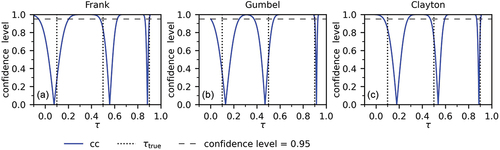
Figure 2 shows that, in principle, a confidence curve for $\mathit{\tau }$ contains more information than one confidence interval for a single confidence level. It also shows that, as ${\tau }_{\mathrm{true}}$ increases, the widths of the confidence intervals that make up the curve decrease. However, Fig. 5 shows that the actual coverage for high ${\tau }_{\mathrm{true}}$ is permissive, so part of the decrease may be due to an underestimation of the interval width. Figure 3 shows that some of the decrease is real.

Figure 3. Box plots of $\hat{\tau }-{\mathit{\tau }}_{\mathrm{true}}$ for different copulas and different sample sizes.

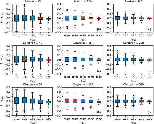
3.3 Spread in the estimate of Kendall’s τ

The box plots in Fig. 3 show that for $\hat{\tau }-{\tau }_{\mathrm{true}}$ both the spread of the outliers and the interquartile distance decrease with increasing sample length for all copulas. The spread of the outliers and the interquartile distance for $\hat{\tau }-{\tau }_{\mathrm{true}}$ also decrease with increasing $\mathit{\tau }$.

This decrease in spread may be caused by the high correlation associated with high $\mathit{\tau }$ values. However, as shown by Fig. 4, the spread in the copula parameter increases with increasing parameter values. The non-linear relation between $\mathit{\theta }$ and $\mathit{\tau }$ and between $\mathit{\theta }$ and the copula shape make it difficult to determine what the actual variation in the copula shape is for a given variation in $\mathit{\tau }$.

Figure 4. Box plots of $\left(\widehat{\theta }-{\theta }_{\text{true}}\right)$ for different copulas and different sample sizes.

3.4 Actual coverage probability for Kendall’s τ

The actual coverage of the confidence interval associated with the confidence curve was examined for all confidence levels. The actual versus nominal coverage probability for random copula samples is shown in Fig. 5, and the coverage at the 95% confidence level is listed in Table 3. According to the results shown in Fig. 5, sample length has little effect on the actual coverage probability up to $\mathit{\tau }=0.5$, and the actual coverage probability does not change much when n increases from 50 to 200. For $\mathit{\tau }=0.9$, the sample length has a visible effect on the actual coverage probability for the Frank and Gumbel copulas but not for the Clayton copula (Fig. 5(g)–(i)).

Table 3. Actual coverage probability (%) of a confidence interval with a nominal coverage probability of 95%.

Copula	τ n	$0.1$	$0.3$	$0.5$	$0.7$	$0.9$
Frank	$50$	$94.2$	$92.6$	$93.1$	$91.5$	$73.0$
	$100$	$95.0$	$93.2$	$92.6$	$92.0$	$84.6$
	$200$	$94.4$	$94.6$	$93.3$	$93.6$	$86.5$
Gumbel	$50$	$94.3$	$90.6$	$87.2$	$84.1$	$72.1$
	$100$	$94.0$	$90.2$	$87.4$	$85.5$	$74.6$
	$200$	$94.7$	$89.8$	$88.0$	$84.6$	$78.1$
Clayton	$50$	$92.0$	$86.5$	$85.1$	$78.5$	$62.3$
	$100$	$92.1$	$86.2$	$83.7$	$81.5$	$63.4$
	$200$	$93.1$	$88.1$	$82.6$	$79.4$	$64.1$

Figure 5. Actual coverage probability versus the nominal one for $\mathit{\tau }$ in copulas.

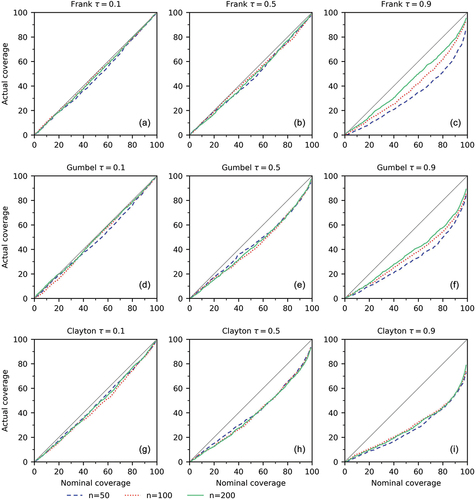
The dependence level strongly influences the coverage. If the samples are weakly dependent, for instance when $\mathit{\tau }=0.1$, then the actual coverage probability is close to nominal (Fig. 5(a), (d), (g)). For samples with high dependence, for instance for $\mathit{\tau }=0.9$, the actual coverage probability is lower than the nominal (Fig. 5(c), (f), (i)).

For bivariate samples from a Frank copula with $\mathit{\tau }=0.9$ and nominal coverage probability of 95%, the actual coverage probability is only 73% for n = 50, 84.6% for n = 100, and 86.5% for n = 200. Results are similar for the other copulas (Table 3).

The statistics for $\hat{\tau }-{\tau }_{\mathrm{true}}$ in Fig. 3 show that the error in the estimate of $\mathit{\tau }$ decreases with increasing ${\tau }_{\mathrm{true}}$. The results in Fig. 3 are in line with this, but Fig. 5 shows that the interval widths for high $\mathit{\tau }$ are overly optimistic. So, while strong dependence is associated with lower uncertainty, the approximate confidence curves calculated by the current version of our code are too optimistic for values of $\mathit{\tau }$ close to 1. Better coverage could perhaps be obtained by using the techniques suggested in Schweder and Hjort (2016) to improve the accuracy of the approximation of the confidence curve.

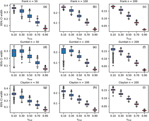
3.5 The width of 95% confidence intervals for the dependence parameter in copulas

Information on the distribution of the widths of the 95% confidence intervals is shown in Fig. 6. The figure shows that the sample length n has a significant effect: the interval width decreases as n gets larger. Therefore, the uncertainty about $\hat{\tau }$ decreases as the sample length gets larger. These results are in qualitative agreement with those shown in Fig. 3.

Figure 6. Box plots of the width of confidence intervals for a 95% confidence level.

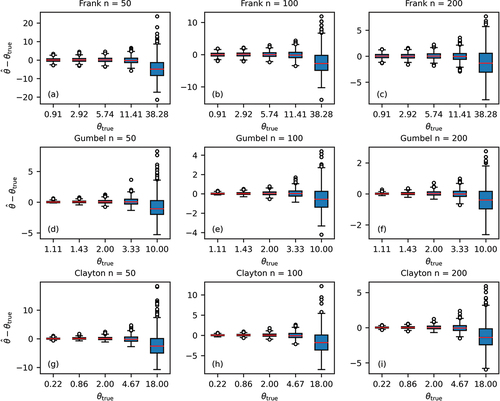
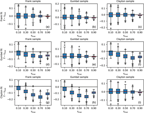
3.6 Effects of the mis-specification of copula

Box plots of the difference between the true value and the estimate of $\mathit{\tau }$ in the synthetic experiments are given in Fig. 7. If the Clayton or Gumbel copula was used to fit a sample from one of the other copula families and calculate, then this resulted in a biased estimate (Fig. 7(d), (f), (g), (h)). The Frank copula did much better in this respect (Fig. 7(a)–(c)). While it is not unexpected that mis-specification has an adverse effect, because of the different shape of the three copulas, it is still worth noting that the Frank copula provides a good estimate of $\mathit{\tau }$, even when applied to a Gumbel or Clayton copula, while the reverse does not hold.

Figure 7. Box plots of the difference between the true value and the estimate of τ in the synthetic experiments with n = 200.

4 Two examples of the use of the method on observed hydrological time series

The method introduced in this study can be used to examine the uncertainty about dependence between time series and the effects of this uncertainty on an analysis based on that dependence. Two examples are given. In the first example the method is used to show the uncertainty about the dependence structure for yearly extremes for several pairs of measurement stations on the Rhine River and its tributaries. The second example investigates estimating the lag between rainfall and runoff for a karst area and the uncertainty in that estimate.

4.1 The relation between time series of annual maxima in the Rhine and its tributaries

In this section the dependency structure of annual minimum or maximum flows will be examined. This structure can be used to answers questions such as

1. What is the probability that high flows will occur in different parts of the same catchment within a given year? This question may be of interest from an insurance, government budget, or disaster preparation point of view.

2. If only series of annual maximum flows are available for branches of a given river system, then can these series provide any information about links between high flows upstream and high flow downstream? If only a time series of annual maximum flows is available, without dates of occurrence, then the probability that two flows will augment each other cannot be determined. However, the probability of a combination of two high flows in the same year is a definite upper bound on the probability that they would combine to generate high discharges downstream. The accuracy of the approximation depends on the way the yearly maximum is determined.

3. If only series of annual minimum flows are available, then can these series provide any information about navigability of the system?

4. Are all parts of the catchment responding in the same way to climate change? In this case dependence between yearly statistics should not change from one period to another.

4.1.1 Methodology used to examine uncertainty of the dependency of return periods

The mapping from annual maximum flows to return periods is a strictly increasing function. In Section 2.1 it was shown that due to the preparatory step for the fitting method used in this article, mapping discharges to return periods or vice versa will not change the result of the fitting process. This implies that using the fitting method to determine the copula parameters for the three different copulas and the associated uncertainty will tell us something about the dependence structure of the return periods. More specifically, are high return periods correlated, and if yes, then how? For the corresponding copula, this would mean that there should be a peak in the pdf in the upper right hand corner of the (u,v) plane. The uncertainty in the dependence structure can be examined by looking at the copula corresponding to the estimated parameter and the difference between that copula and copulas corresponding to the lower or upper bound of a confidence interval for a given confidence level.

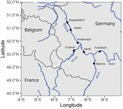
Time series of annual daily maximum flows for several stations for the Rhine and one station each for the Mosel and the Main were obtained from the Global Runoff Data Center (GRDC 2021). The stations are shown in Fig. 8. As the time series are series of annual maxima, a copula package by Hofert et al. (2020) was used to extend the collection of one-parameter copulas applied to the series with additional copulas specifically suited for extreme values: Galambos and Huesler-Reiss (Appendix C.2). Of the other extreme value copulas, the Tawn copula was not considered because it is limited to values for Kendall’s $\mathit{\tau }$ below 0.418, and the t-EV copula was not considered because it has two parameters. To allow for high correlation both for low and for high return periods, the copulas that have different correlation structure for low and high parameters (Clayton, Gumbel, Galambos, Huesler-Reiss) were tried both in their standard orientation and after a 180 degree rotation; the rotated copula will be denoted by adding “180°” after the copula name. As in the rest of the paper, the uncertainty in the parameter is represented by a confidence curve for Kendall’s $\mathit{\tau }$. For a given $\mathit{\tau }$, the shape of the Galambos and Huesler-Reiss copulas is very close to that of the Gumbel copula.

Figure 8. Station locations.

4.1.2 Results found for uncertainty in dependency structure of return periods

To illustrate the type of results that would be obtained, four pairs of measurement stations were selected that were expected to have different dependency structures. For each pair the discharge at a station downstream of the confluence point was determined. The pair Andernach and Koeln serves as a test case. For these stations a near perfect correlation was expected because no major tributaries enter the river between the stations. Figure 9(a) confirms this. Figure 9(b) shows that high discharges at the downstream station tend to be correlated as well. Values of the parameter $\mathit{\theta }$ and $\mathit{\tau }$ values can be found in Tables 4 and 5, respectively. The other station pairs combine a station on a tributary with a station on the Rhine upstream of the confluence. All pairs show definite correlation, as the bounds of the confidence intervals up to 99% are well away from zero (Fig. 9(b)–(d)). For all pairs the best fit was obtained with the version of Gumbel, Galambos or Huesler-Reiss that is rotated 180° around the point (0.5,0.5) in the (u,v) plane. Given the shape of the pdf of these copulas, with a peak in the lower left quadrant, this could suggest stronger correlation for short return periods than for long return periods. However, the scarcity of points in the upper right corner could also have caused this preference for the rotated version (Fig. 9(f)–(h)).

Table 4. Dependence parameters between time series and width of the 95% confidence intervals for the estimate of dependence parameter.

Time series pair	Frank		Clayton		Gumbel ${180}^{\circ }$		Galambos ${180}^{\circ }$		Huesler-Reiss ${180}^{\circ }$
	$\mathit{\theta }$	Width	$\mathit{\theta }$	Width	$\mathit{\theta }$	Width	$\mathit{\theta }$	Width	$\mathit{\theta }$	Width
Andernach and Koeln	59.0	21.7	20.3	7.8	14.7	5.1	14.0	5.1	16.4	5.0
Cochem and Kaub	8.0	3.8	2.3	1.3	2.5	0.9	1.8	0.9	2.2	0.8
Cochem and Worms	5.4	3.2	1.5	1.0	1.9	0.7	1.2	0.6	1.7	0.7
Worms and Frankfurt	4.6	3.8	1.2	1.1	1.7	0.7	1.0	0.7	1.5	0.8

Table 5. Kendall’s $\mathit{\tau }$ values between time series and width of the 95% confidence intervals.

Time series pair	Frank		Clayton		Gumbel ${180}^{\circ }$		Galambos ${180}^{\circ }$		Huesler-Reiss ${180}^{\circ }$
	$\mathit{\tau }$	Width	$\mathit{\tau }$	Width	$\mathit{\tau }$	Width	$\mathit{\tau }$	Width	$\mathit{\tau }$	Width
Andernach and Koeln	0.93	0.02	0.91	0.03	0.93	0.02	0.93	0.02	0.93	0.02
Cochem and Kaub	0.60	0.14	0.53	0.14	0.60	0.14	0.60	0.14	0.58	0.13
Cochem and Worms	0.48	0.19	0.43	0.16	0.48	0.18	0.48	0.18	0.47	0.16
Worms and Frankfurt	0.43	0.26	0.37	0.22	0.42	0.25	0.42	0.24	0.42	0.23

Figure 9. Confidence curves and scatter plots for pairs of stations. Discharge at the downstream station is indicated by the colour of the dots in the scatter plots.

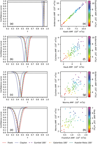
In the scatter plots (Fig. 9(e)–(h)) colour is used to show the discharge at a station downstream of the confluence of tributary and main river. These plots were added to show that even the (at first sight oversimplified) approach of looking for dependence between high discharges in the same calendar year may provide at least some information on high flows.

An illustration of the variation in shape of the pdf of a copula over a 95% confidence interval can be found in Fig. 10 for the pair Cochem and Kaub. For example, for the Frank copula Fig. 10(a) shows the pdf for $\hat{\theta }$; Fig. 10(f) shows the difference between the pdf at $\hat{\theta }$ and the pdf at the lower bound of the confidence interval, and Fig. 10(k) shows the difference between the pdf at $\hat{\theta }$ and the pdf at the upper bound of the confidence interval. Similar plots are shown for the other copulas.

Figure 10. The pdfs for copulas for the station pair Cochem and Kaub.

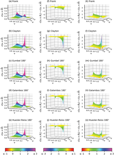
The confidence curves provide the variation in the copula at different confidence levels and therefore provide insight into the effect of uncertainty on specific joint return times. While the whole upper quadrant ([0.5,1] × [0.5,1]) would be of interest, limitations deriving from viewing three-dimensional information in two dimensions usually lead to examination of exceedance frequencies or, equivalently, return periods. The relation between return periods and copulas is discussed by Salvadori et al. (2007, sec. 3.3). For instance, the probability that in a specific year the discharges in both rivers are in the top 10% of return periods corresponds with the integral of the pdf of the copula over the rectangle [0.9,1] × [0.9,1], which corresponds to the value $\bar{C}\left(1-0.9,1-0.9\right)$ where

(11) $\bar{C}\left(\mathit{u},\mathit{v}\right)=\mathit{u}+\mathit{v}-1+\mathit{C}\left(1-\mathit{u},1-\mathit{v}\right)$(11)

which relates to a return period by ${\mu }_T/\bar{C}\left(1-0.9,1-0.9\right)$, where ${\mu }_T$ is the the mean inter-arrival time (for annual maxima this is one year). We can now relate the copula to return periods for combined ${\mu }_T/\left(1-\mathit{u}\right)$, ${\mu }_T/\left(1-\mathit{v}\right)$ floods. The confidence curve allows us to pick a copula parameter range associated with a given confidence level. As a result, we get a confidence interval for the return period of two floods within the same year.

4.2 Dependence structure between rainfall and discharge for a karst area

The relation between rainfall onto and runoff out of a catchment is determined by physical processes and therefore it is a deterministic one. However, there is considerable epistemic uncertainty about the processes and their parameters. As a result, the relation between rainfall and runoff may seem to be different at different times. The simplest possible deterministic model for this relation would be one in which the runoff is a shifted and scaled version of the rainfall. A first improvement would be replacement of the simple scaling relationship by a joint distribution of runoff and shifted rainfall. The model would be constructed by fitting a dependence structure to the shifted rain and the runoff for a range of shifts. The shift would be chosen by assuming that the dependence would be strongest for a shift that best corresponded to the delay between rainfall and runoff. This approach would only work if the shift could be determined with sufficient certainty. It was decided to investigate the uncertainty in the estimate of the shift with the confidence curve method proposed in this article, using a dataset from the Djebel Zaghouan region in Tunisia.

The Djebel Zaghouan is the most important Jurassic formation of the Zaghouan massif and lies about 50 km to the south of Tunis. The massif consists mainly of overlapping limestone monoclines. It is also contains marls of the Cretaceous and Eocene (Castany 1951). The Djebel Zaghouan is characterized by the presence of southern and transverse faults that have created blocks (Ferjani et al. 2020). These faults facilitate infiltration. The Zaghouan karst aquifer covers an area of approximately 19.6 km² (Fig. 11). In the eastern part, conditions are favourable for the storage of seepage water, whereas in the western part marl deposits result in a much lower storage coefficient (Djebbi et al. 2001).

Figure 11. Location of the karst area. Both figures combine Google Map data ©2015 with material from Natural Earth.

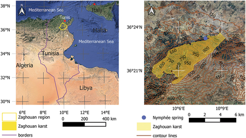
The Zaghouan region lies on the border between the upper semi-arid and the sub-humid climate zones. It is characterized by an average annual rainfall of 467 mm (values ranging from 245 to 625 mm) with a heterogeneous spatial and temporal distribution. Rainfall measurements were taken on a daily basis at the “Zaghouan controle” station (latitude: 36.39583N; longitude: 10.14917E) during the period from 1915 to 1944. However, there are gaps in the data for the entire year of 1929 and for January 1930. These gaps were filled by using data from the nearby station “Zaghouan SM” (latitude: 36.40306N; longitude: 10.14472E). This resulted in a complete series of daily and weekly cumulative rainfall. The discharge series used was recorded from 1915 to 1943 at the Nymphée spring. It was originally recorded in graphical form only. Measurements were taken at irregular intervals with frequencies varying from twice weekly to monthly. To extract information, the graphical data was digitized. The time series contains two atypical years: a very wet one during the hydrological year running from September 1920 to August 1921 and a relatively dry hydrological year starting in 1926. These resulted in total volumes of 6.5 × 10⁶ m³ and 1.9 × 10⁶ m³, respectively. A fragment of the original document from the archive of hydrological yearbooks of the General Directorate of Water Resources (abbreviated DGRE, in French) containing the hydrograph (curve) from 1924 to 1926 is shown in Fig. 12. Major engineering works were performed in 1944, but the data from 1915 to 1943 reflects the natural flow conditions.

Figure 12. The hydrograph (curve) for Nymphée spring from 1924 to 1926. The figure also contains a monthly hyetograph (bars).

These observations are consistent with the natural flow of the resurgences during this period. According to the criteria in Olarinoye et al. (2020), the accuracy and quality of the hydrograph is class A: the discharge observation measurement is known, recognition of individual events on the spring’s hydrograph, recognition of seasonal events on the spring’s hydrograph, and identification of recession events on the hydrograph (see Fig. 12). The karst falls into class 6 as defined by Cinkus et al. (2021) in the Karst Aquifer Resources availability and quality in the Mediterranean Area (KARMA) project. The karst has a minimum inertia of two months, so it was deemed appropriate to acquire consistent time series of daily, weekly, and monthly flows by linear interpolation. The daily flow series was used primarily to test the algorithm. Today, the aquifer is fully exploited to provide drinking water to the city of Zaghouan. Unfortunately, this overexploitation has hindered the natural reemergence of springs in this region for many years.

4.2.1 Methodology used to determine the shift between rainfall and runoff

The lag between rainfall and runoff was estimated by fitting copulas to the rainfall time series and a version of the runoff series that was shifted by m steps for m ranging from 0 up to $m_{\max }$. To avoid artefacts due to different time series lengths for different lags, the last $m_{\max }$ points of the rainfall time series were dropped and the shifted runoff series length was adjusted to match. Different copulas were fitted to see if this made an appreciable difference in the results. The lag was estimated by

$\hat{m}=\arg \underset{\theta }{max}\hat{\theta }\left(\mathit{m}\right)$

where $\hat{\theta }\left(\mathit{m}\right)$ is the estimate of the copula parameter. The pmle is asymptotically normal (Genest et al. 1995). An estimate of the standard deviation of this normal distribution was obtained by taking the 95% confidence interval and translating this into a standard deviation for the normal distribution. For selected values, this was checked against calculations using the R copula package, which gave very similar results but took much longer to perform the calculations and sometimes ran into problems when the procedure did not converge. The lag estimate was used to get bounds on the lag as follows:

1. Construct an interval $\left[m_0,m_1\right]$ around $\text{hatm}$ on which $\hat{\tau }\left(\mathit{m}\right)$, the Kendall’s $\mathit{\tau }$ value corresponding to $\hat{\theta }\left(\mathit{m}\right)$, is strictly positive.

2. For each $\mathit{m}\in \left\{m_0,m_0+1,\dots ,m_1\right\}$ use the confidence curve for $\hat{\theta }\left(\mathit{m}\right)$ to get the 95% confidence interval width $w_{95}\left(\mathit{m}\right)$.

3. For each m draw random values ${\theta }_{\mathit{i},\mathit{m}}$, $\mathit{i}=1,2,\dots ,n_{\mathrm{R}}$ ($n_{\mathrm{R}}=10000$) from the normal distribution with mean $\hat{\theta }\left(\mathit{m}\right)$ and standard deviation $\mathit{\sigma }\left(\mathit{m}\right)=w_{95}\left(\mathit{m}\right)/3.92$. Here, 3.92 is the approximate width of the 95% confidence interval for the standard normal distribution. This results in $n_{\mathrm{R}}\times \left(m_1-m_0+1\right)$ values ${\theta }_{\mathit{i},\mathit{m}}$.

4. For all ${\theta }_{\mathit{i},\mathit{m}}$, calculate the corresponding values ${\tau }_{\mathit{i},\mathit{m}}$.

5. For each i, determine the lag corresponding to the maximum value of ${\tau }_{\mathit{i},\mathit{m}}$ and label this ${\hat{m}}_{\mathit{i}}$. Use the cdf of the ${\hat{m}}_{\mathit{i}}$ to determine the bounds of a confidence interval for the lag. This procedure ignores the constraint that the curve should have exactly one local maximum in $\left[m_0,m_1\right]$ and is therefore probably on the conservative side.

4.2.2 Results found for the lag

Figure 13 shows daily rainfall and runoff for the karst area. In addition, a line is plotted representing the runoff shifted backward in time over a number of days corresponding to the estimated lag. Frank, Gumbel, and Clayton confidence curves for $\hat{\tau }\left(\hat{m}\right)$ are shown in Fig. 14(a), (c), and (e) for time steps of one day, one week, and one month, respectively. The results for a time step of one day served mainly to test the algorithm.

Figure 13. Daily rainfall, runoff, and shifted runoff.

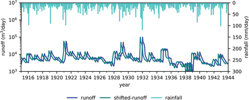
Figure 14. Kendall’s τ for different lags and confidence curves for the selected lag (CI = confidence interval).

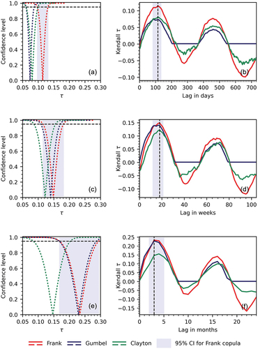
The curves of $\hat{\tau }\left(\mathit{m}\right)$ versus the lag m for Frank, Gumbel, and Clayton are shown in Fig. 14(b), (d), and (f) for time steps of one day, one week, and one month, respectively. The estimated lag and confidence interval are shown for the Frank copula only. Please note that the Gumbel copula can only model positive correlations, so a result of zero was returned when the dependence would result in a negative $\mathit{\tau }$. The Frank copula consistently delivered the highest values. Lags of about 3 to 4 months were found at all temporal scales. Table 6 provides values of the lag estimates and the 90% and 95% confidence intervals for these estimates. The confidence intervals show that the results for all time scales and all copulas are compatible. This was in accordance with results obtained with the conceptual KarstMod model and with neural networks in the KARMA project (Mazzilli et al. 2019, KARMA 2021).

Table 6. Table of lags and confidence intervals.

Copula	Time step	$\hat{\tau }\left(\hat{m}\right)$	$\hat{m}$	90% interval	95% interval
Frank	Day	0.114	115	[86.0, 131.0]	[83.0, 133.0]
	Week	0.149	18	[13.0, 20.0]	[12.0, 21.0]
	Month	0.233	3	[3.0, 5.0]	[2.0, 5.0]
Clayton	Day	0.081	116	[85.0, 136.0]	[82.0, 141.0]
	Week	0.122	18	[13.0, 21.0]	[12.0, 22.0]
	Month	0.156	4	[3.0, 5.0]	[3.0, 6.0]
Gumbel	Day	0.074	87	[78.0, 125.0]	[75.0, 128.0]
	Week	0.140	17	[11.0, 19.0]	[11.0, 20.0]
	Month	0.229	3	[2.0, 4.0]	[2.0, 5.0]

5 Conclusions

In this article, a new method was developed that uses confidence curves as a means to represent epistemic uncertainty in the estimate of the copula parameter for one-parameter copulas. A pseudo maximum likelihood estimator (pmle), denoted by $\hat{\theta }$, was used to estimate the copula parameter $\mathit{\theta }$ for synthetic and real data. For the copulas used here, there is a one-to-one correspondence between the $\mathit{\theta }$ and Kendall’s $\mathit{\tau }$ that respects ordering. This allows better comparison between results of different copulas and a more convenient interpretation, so the parameter $\mathit{\theta }$ of each copula was transformed into the corresponding $\mathit{\tau }$ and $\hat{\theta }$ was transformed into $\hat{\tau }$.

Confidence curves have the advantage that they offer much more information than just one confidence interval. In fact, they offer about the same amount of information as an a posteriori Bayes distribution, but without the need to first find the correct prior. In hydrology, such information is especially important because the decisions based on hydrological analyses usually have a large impact, and the questions posed can rarely be adequately answered with a simple yes or no. A confidence curve allows the exploration of a range of answers based on different levels of confidence.

Statistical analysis of confidence curves constructed from synthetic time series resulted in the following findings:

1. For all copulas a box plot showed that $\hat{\tau }-{\tau }_{\mathrm{true}}$ decreased with increasing time series length and with increasing $\mathit{\tau }$. Here, ${\tau }_{\mathrm{true}}$ is used to denote the $\mathit{\tau }$ of the copula used to generate the sample. The results suggest that the pmle estimator gives an acceptable performance.

2. For all copulas a comparison of actual and nominal coverage shows that the confidence curves are permissive, especially for $\mathit{\tau }>0.5$. This could be addressed by using techniques suggested by Schweder and Hjort (2016).

3. For all copulas, the width of the 95% confidence interval decreased with increasing time series length and increasing $\mathit{\tau }$. The results suggest that this interval is of a reasonable size, although the results for $\mathit{\tau }>0.5$ show sizes that still need to be corrected for the permissive coverage.

4. The pmle for the Frank copula provided good estimates for $\mathit{\tau }$ even for samples from the Gumbel and Clayton copula.

For the Rhine River case study, two results stand out. Firstly, all extreme value copulas fit best when rotated 180°, and, secondly, the parameter estimate and the confidence curve for Kendall’s $\mathit{\tau }$ delivered by the Frank copula are very close to the estimates and the confidence curves corresponding to the extreme value copulas. This suggests that the effect observed for synthetic data, namely that Frank seemed to give good results for Kendall’s $\mathit{\tau }$ even when the time series was drawn from another copula, may well extend to real time series.

For the Tunisian karst region, the pmle estimate was mapped to a $\mathit{\tau }$ value, and this was used to estimate the lag between rainfall and runoff. The confidence curve for the $\mathit{\tau }$ corresponding to the chosen lag served as an initial check on the relevance of the correlation. It was also used to approximate the distribution of the points on the curve of the estimated $\hat{\tau }\left(\mathit{m}\right)$ versus the lag m. This in turn allowed the generation of alternative curves and an estimate of a confidence interval for the lag. The lag found was in accordance with results of earlier research. As the Gumbel copula cannot model negative correlations, this copula gave no results when the actual correlation was negative. When calculating $\mathit{\tau }$ for the different lags, the Frank copula gave values that were larger in magnitude than the Clayton and Gumbel copulas. The delays found are in accordance with the results obtained with the conceptual KarstMod model and with neural networks in the KARMA project (Mazzilli et al. 2019, KARMA 2021).

In both cases, the confidence curves for the copula parameter allowed simple propagation of the uncertainty in the parameter to quantities of direct hydrological significance, and in both cases, the Frank copula gave the highest estimate for Kendall’s $\mathit{\tau }$.

All results show that confidence curves for copula parameters are a valuable addition to the hydrological tool set and can be used in a wide variety of hydrological settings. Earlier work already showed the value of confidence curves for change point analysis (Zhou et al. 2020, 2023). In certain cases confidence curves may provide an alternative to Bayesian methods. Further research is planned to see whether the coverage can be corrected either by a correction factor, as suggested for a more general case by Schweder and Hjort (2016), or through the use of Monte Carlo simulation to generate an approximate probability distribution for the deviance.

Acknowledgements

This work was partially developed within the framework of the Panta Rhei research initiative (Montanari etal. 2013, McMillan etal. 2016) of the International Association of Hydrological Sciences (IAHS) by members of the working group on ‘Natural and man-made control systems in water resources’. The authors thank the Regional Commissariat for Agricultural Development of Zaghouan (CRDA Zaghouan) for providing the rainfall–runoff data for the Zaghouan karst region.

Disclosure statement

No potential conflict of interest was reported by the authors.

Additional information

Funding

This work was supported by the China Scholarship Council under Grant number [201706710004]. The research concerning the Tunisian karst region was supported by the Partnership for Research and Innovation in the Mediterranean Area (PRIMA) programme under Horizon 2020 (KARMA project, grant agreement number [01DH19022A]).

Appendices Appendix A.

Notations and definitions

The probability of a given event E is denoted by Pr(E). The indicator function is a very useful function in statistics, but the notation used for it varies widely. In this article, an abbreviated form of the traditional notation is used. If A is a set, then the indicator function $1_A\left(\mathit{x}\right)$ is 1 for elements of A and 0 elsewhere:

(A1) ${\mathbf{1}}_A\left(\mathit{x}\right)=\{\begin{array}{cc}1& \mathrm{if}\mathit{x}\in \mathit{A}\\ 0& \mathrm{if}\mathit{x}\notin \mathit{A}\end{array}$(A1)

In probability theory, it is often applied to RVs with as set an interval like $\left(-\mathrm{\infty },\mathit{x}\right]$; in that case the following abbreviation is used:

$1_{\underset{\_}{x}\le \mathit{x}}=1_{\left(-\mathrm{\infty },\mathit{x}\right]}\left(\underset{\_}{x}\right)$

Let $\underset{\_}{\mathit{Z}}=\left({\underset{\_}{\mathit{z}}}_1,{\underset{\_}{\mathit{z}}}_2,\dots ,{\underset{\_}{\mathit{z}}}_{\mathit{n}}\right)$ be a random sample of size n where the ${\underset{\_}{\mathbf{z}}}_{\mathit{i}}$ are independent identically distributed random vectors, and $\mathit{Z}=\left({\mathit{z}}_1,{\mathit{z}}_2,\dots ,{\mathit{z}}_n\right)$ a realization of such a sample. In the following definitions, $\mathit{\lambda }$ is a property of the distribution of ${\underset{\_}{\mathit{z}}}_{\mathit{i}}$ that can be expressed as a real number; it can be one of the distribution parameters, one of its moments, or perhaps a specific quantile.

Definition 1. A confidence set for $\mathit{\lambda }$ at a given confidence level $\mathit{\gamma }$ is a set valued function $\mathit{R}\left(\mathit{Z}\right)$ such that for the true value ${\lambda }_{\mathrm{true}}$ of $\mathit{\lambda }$ the expression $\mathit{R}\left(\underset{\_}{\mathit{Z}}\right)$ is a random set that satisfies

(A2) $\mathrm{Pr}\left({\lambda }_{\mathrm{true}}\in \mathit{R}\left(\underset{\_}{\mathit{Z}}\right)\right)=\mathit{\gamma }$(A2)

The value $\mathit{\gamma }$ is the nominal coverage probability. In practice, (A2) may not hold exactly, either because it holds only when the sample size n tends to infinity, or because it was derived under assumptions on the sample that are only approximately satisfied during the experiment. The actual coverage probability of a confidence interval is the probability of the confidence interval containing the true value of a statistic $\mathit{\lambda }$ in the experiment as it was performed. A confidence interval is a special case of a confidence set.

Definition 2. If f is a function from $\mathbb{R}$ to $\mathbb{R}$, then a sub-level set of f at level $\mathit{\gamma }$ is a set

(A3) $\left\{\mathit{t}\in \mathbb{R}:\mathit{f}\left(\mathit{t}\right)\le \mathit{\gamma }\right\}$(A3)

Definition 3. A confidence curve is a function $\mathrm{cc}\left(\mathit{\lambda },\mathit{Z}\right)$ from $\mathbb{R}\times {\mathbb{R}}^{\mathit{k}\times \mathit{n}}$ to [0,1] that satisfies the following conditions (Schweder and Hjort 2016, Definition 4.3):

1. The sub-level set of $\mathrm{cc}\left(\mathit{\lambda },\mathit{Z}\right)$ at level $\mathit{\gamma }$ is a confidence set for $\mathit{\lambda }$ at the confidence level $\mathit{\gamma }$, so

   $\mathrm{Pr}\left({\lambda }_{\mathrm{true}}\in \left\{\mathit{\lambda }:\mathrm{cc}\left(\mathit{\lambda },\mathit{Z}\right)\le \mathit{\gamma }\right\}\right)=\mathit{\gamma }$

2. There is a function $\hat{\lambda }\left(\mathit{Z}\right)$ from ${\mathbb{R}}^{\mathit{k}\times \mathit{n}}$ to $\mathbb{R}$ such that the RV $\hat{\lambda }\left(\underset{\_}{\mathit{Z}}\right)$ is a point estimator for $\mathit{\lambda }$.

3. For all realizations ${\mathit{Z}}_{\mathrm{obs}}$ of a random sample $\underset{\_}{\mathit{Z}}$, $\underset{\lambda }{min}\mathrm{cc}\left(\mathit{\lambda },{\mathit{Z}}_{\mathrm{obs}}\right)=\mathrm{cc}\left(\hat{\lambda }\left({\mathit{Z}}_{\mathrm{obs}}\right),{\mathit{Z}}_{\mathrm{obs}}\right)=0$

4. For the true value ${\lambda }_{\mathrm{true}}$ of $\mathit{\lambda }$, the RV $\mathrm{cc}\left({\lambda }_{\mathrm{true}},\underset{\_}{\mathit{Z}}\right)$ has a uniform distribution on the unit interval.

For a confidence curve $\mathrm{cc}$, the actual coverage probability of a confidence interval at a confidence level of $\mathit{\gamma }$ for a sample of size n can be estimated by

(A4) $\frac{1}{n}\sum _{\mathit{i}=1}^n{1}_{\mathrm{cc}\left({\mathit{\lambda }}_{\mathrm{true}},{\mathit{z}}_{\mathrm{obs},i}\right)\le \mathit{\gamma }}$(A4)

It should be close to the nominal coverage probability $\mathit{\gamma }$.

Appendix B.

An uninformative confidence interval for τ

It is known that $\mathit{\tau }\in \left[-1,1\right]$. Now suppose that $\mathit{\gamma }\in \left(0,1\right)$ and there is no a priori information on the location of $\mathit{\tau }$. If a point y is selected at random in the interval $\left[-1,1-2\mathit{\gamma }\right]$, then

$\begin{array}{cc}\mathrm{Pr}\left(\mathit{\tau }\in \left[\mathit{y},\mathit{y}+2\mathit{\gamma }\right]\right)& =\underset{\mathit{x}=-1}{\overset{1}{\int }}\underset{\mathit{y}=-1}{\overset{1-2\mathit{\gamma }}{\int }}{1}_{\mathit{y}\le \mathit{x}\le \mathit{y}+2\mathit{\gamma }}\frac{1}{2}\mathit{dx}\frac{1}{2-2\mathit{\gamma }}\mathit{dy}\\ \mathit{\hspace{0.17em}}& =\frac{1}{4\left(1-\mathit{\gamma }\right)}\underset{\mathit{y}=-1}{\overset{1-2\mathit{\gamma }}{\int }}\underset{\mathit{x}=-1}{\overset{1}{\int }}{1}_{\mathit{y}\le \mathit{x}\le \mathit{y}+2\mathit{\gamma }}\mathit{dxdy}\\ \mathit{\hspace{0.17em}}& =\frac{1}{4\left(1-\mathit{\gamma }\right)}\underset{\mathit{y}=-1}{\overset{1-2\mathit{\gamma }}{\int }}\underset{\mathit{x}=\mathit{y}}{\overset{\min \left(\mathit{y}+2\mathit{\gamma },1\right)}{\int }}{1}_{\mathit{y}\le \mathit{x}\le \mathit{y}+2\mathit{\gamma }}\mathit{dxdy}\end{array}$

so

$\begin{array}{cc}\mathrm{Pr}\left(\mathit{\tau }\in \left[\mathit{y},\mathit{y}+2\mathit{\gamma }\right]\right)& =\frac{1}{4\left(1-\mathit{\gamma }\right)}\underset{\mathit{y}=-1}{\overset{1-2\mathit{\gamma }}{\int }}\underset{\mathit{x}=\mathit{y}}{\overset{\mathit{y}+2\mathit{\gamma }}{\int }}\mathit{dxdy}\\ \mathit{\hspace{0.17em}}& =\frac{1}{4\left(1-\mathit{\gamma }\right)}\underset{\mathit{y}=-1}{\overset{1-2\mathit{\gamma }}{\int }}2\mathit{\gamma dy}\\ \mathit{\hspace{0.17em}}& =\frac{1}{4\left(1-\mathit{\gamma }\right)}2\mathit{\gamma }\left(2-2\mathit{\gamma }\right)=\mathit{\gamma }\end{array}$

This implies that, as long as there is no a priori reason to assume the parameter has a certain value, it is possible to obtain a confidence interval at level $\mathit{\gamma }$ without using the sample, as long as an interval length of (at least) $2\mathit{\gamma }$ is allowed.

Appendix C.

Copulas

Copulas were introduced by Sklar (1959). For a modern overview and hydrological examples see, for instance, Salvadori and De Michele (2004, 2007), Favre et al. (2004), or Genest and Favre (2007).

Appendix C.1 Some Archimedean copulas

Appendix C.1.1. Frank copula

The cdf for the Frank copula is

(C1) $C_{\mathrm{F}}\left(\mathit{u},\mathit{v};\mathit{\theta }\right)=-\frac{1}{\theta }\log \left[1+\frac{\left(\exp \left(-\mathit{\theta u}\right)-1\right)\left(\exp \left(-\mathit{\theta v}\right)-1\right)}{\exp \left(-\mathit{\theta }\right)-1}\right]$(C1)

where $-\mathrm{\infty }<\mathit{\theta }<0$ or $0<\mathit{\theta }<\mathrm{\infty }$. The pdf for the Frank copula is

(C1) $c_{\mathrm{F}}\left(\mathit{u},\mathit{v};\mathit{\theta }\right)=\frac{\mathit{\theta }\left(1-\exp \left(-\mathit{\theta }\right)\right)\exp \left(-\mathit{\theta }\left[\mathit{u}+\mathit{v}\right]\right)}{{\left(\exp \left(-\mathit{\theta }\right)-\exp \left(-\mathit{\theta u}\right)-\exp \left(-\mathit{\theta v}\right)+\exp \left(-\mathit{\theta }\left[\mathit{u}+\mathit{v}\right]\right)\right)}^2}$(C1)

Appendix C.1.2. Clayton copula

The cdf for the Clayton copula is

(C3) $C_{\mathrm{C}}\left(\mathit{u},\mathit{v};\mathit{\theta }\right)={\left[\max \left({\mathit{u}}^{-\mathit{\theta }}+v^{-\mathit{\theta }}-1,0\right)\right]}^{-1/\mathit{\theta }}$(C3)

where $-1\le \mathit{\theta }<\mathrm{\infty }$. The pdf for the Clayton copula is

(C4) $c_{\mathrm{C}}\left(\mathit{u},\mathit{v};\mathit{\theta }\right)=\left\{\begin{array}{cc}0& \mathit{\eta }\left(\mathit{u},\mathit{v},\mathit{\theta }\right)<0\\ 0& \mathit{\eta }\left(\mathit{u},\mathit{v},\mathit{\theta }\right)=0,-1<\mathit{\theta }<0\\ \left(1+\mathit{\theta }\right)u^{-1-\mathit{\theta }}{v}^{-1-\mathit{\theta }}\mathit{\eta }{\left(\mathit{u},\mathit{v},\mathit{\theta }\right)}^{-2-1/\theta }& \mathit{\eta }\left(\mathit{u},\mathit{v},\mathit{\theta }\right)>0\end{array}\right.$(C4)

where $\mathit{\eta }\left(\mathit{u},\mathit{v},\mathit{\theta }\right)=u^{-\mathit{\theta }}+v^{-\mathit{\theta }}-1$

Appendix C.1.3. Gumbel copula

The cdf for the Gumbel copula is

(C5) $C_{\mathrm{G}}\left(\mathit{u},\mathit{v};\mathit{\theta }\right)=\exp \left(-{\left[{\left(-\log u\right)}^{\theta }+{\left(-\log v\right)}^{\theta }\right]}^{1/\mathit{\theta }}\right)$(C5)

where $1\le \mathit{\theta }<\mathrm{\infty }$. The pdf for the Gumbel copula is

(C6) $\begin{array}{cc}{c}_{\mathrm{G}}\left(\mathit{u},\mathit{v};\mathit{\theta }\right)& =\frac{{\mathit{C}}_{\mathrm{G}}\left(\mathit{u},\mathit{v};\mathit{\theta }\right)}{\mathit{uv}}{\left(\log u\log v\right)}^{\mathit{\theta }-1}{\left({\left(-\log u\right)}^{\theta }+{\left(-\log v\right)}^{\theta }\right)}^{1/\mathit{\theta }-2}\\ \mathit{\hspace{0.17em}}& \times \left({\left({\left(-\log u\right)}^{\theta }+{\left(-\log v\right)}^{\theta }\right)}^{1/\mathit{\theta }}+\mathit{\theta }-1\right)\end{array}$(C6)

Appendix C.2 Some extreme value copulas

A bivariate extreme value copula is a copula that satisfies

(C7) $\mathit{C}\left(u^n,v^n\right)={\left(\mathit{C}\left(\mathit{u},\mathit{v}\right)\right)}^n,\mathit{n}>0$(C7)

The Gumbel copula described earlier is an extreme value copula.

Appendix C.2.1. Galambos copula

The cdf for the Galambos copula is

(C8) $C_{\mathrm{Ga}}\left(\mathit{u},\mathit{v};\mathit{\theta }\right)=\mathit{uv}\exp \left({\left[{\left(-\log u\right)}^{-\mathit{\theta }}+{\left(-\log v\right)}^{-\mathit{\theta }}\right]}^{-1/\mathit{\theta }}\right)$(C8)

where $0\le \mathit{\theta }<\mathrm{\infty }$.

Appendix C.2.2. Huesler-Reiss copula

The cdf for the Huesler-Reiss copula is

(C9) $C_{\mathrm{HR}}\left(\mathit{u},\mathit{v};\mathit{\theta }\right)=\exp \left[\left(\log \mathit{u}\right)\mathrm{\Phi }\left(\frac{1}{\theta }+\frac{\theta }{2}\log \left(\frac{\log u}{\log v}\right)\right)+\left(\log \mathit{v}\right)\mathrm{\Phi }\left(\frac{1}{\theta }+\frac{\theta }{2}\log \left(\frac{\log v}{\log u}\right)\right)\right]$(C9)

where $0\le \mathit{\theta }<\mathrm{\infty }$ and $\mathrm{\Phi }$ is the cdf of the univariate standard normal distribution.

References

- Abramowitz, M. and Stegun, I.A., 1970. Handbook of mathematical functions. New York: Dover Publications Inc.
- Bayarri, M.J. and Berger, J.O., 2004. The interplay of Bayesian and frequentist analysis. Statistical Science, 19 (1), 58–80. doi:10.1214/088342304000000116.
- Blöschl, G., et al., 2019. Twenty-three Unsolved Problems in Hydrology (UPH) – a community perspective. Hydrological Sciences Journal, 64 (10), 1141–1158. doi:10.1080/02626667.2019.1620507.
- Castany, G., 1951. Geological study of the Tunisian Eastern Atlas. Besançon: Imp de l’IEST.
- Chen, X. and Fan, Y., 2005. Pseudo-likelihood ratio tests for semiparametric multivariate copula model selection. Canadian Journal of Statistics, 33 (3), 389–414. doi:10.1002/cjs.5540330306.
- Cinkus, G., Mazzilli, N., and Jourde, H., 2021. Identification of relevant indicators for the assessment of karst systems hydrological functioning: proposal of a new classification. Journal of Hydrology, 603 (December), 127006. doi:10.1016/j.jhydrol.2021.127006.
- Cunen, C. and Hjort, N.L., 2021. Combining information across diverse sources: the II-CC-FF paradigm. Scandinavian Journal of Statistics, 49 (2), 625–656. doi:10.1111/sjos.12530.
- Djebbi, M., et al., 2001. Les sources karstiques de Zaghouan. Recherche d’un opérateur pluie-débit. In: Conference on limestone hydrology and fissured media, 125–128.
- Favre, A.C., et al., 2004. Multivariate hydrological frequency analysis using copulas. Water Resources Research, 40 (1). doi:10.1029/2003wr002456.
- Ferjani, A.H., et al., 2020. Enhanced characterization of water resource potential in Zaghouan region, Northeast Tunisia. Natural Resources Research, 29 (5), 3253–3274. doi:10.1007/s11053-020-09647-x.
- Genest, C. and Favre, A.C., 2007. Everything you always wanted to know about copula modeling but were afraid to ask. Journal of Hydrologic Engineering, 12 (4), 347–368. doi:10.1061/(ASCE)1084-0699(2007)12:4(347).
- Genest, C., Ghoudi, K., and Rivest, L.P., 1995. A semiparametric estimation procedure of dependence parameters in multivariate families of distributions. Biometrika, 82 (3), 543–552. doi:10.1093/biomet/82.3.543.
- GRDC, 2021. Long-term statistics and annual characteristics of GRDC timeseries data. The Global Runoff Data Centre, 56068 Koblenz, Germany. Available from: https://www.bafg.de/GRDC.
- Hemelrijk, J., 1966. Underlining random variables. Statistica Neerlandica, 20 (1), 1–7. doi:10.1111/j.1467-9574.1966.tb00488.x.
- Hofert, M., et al, 2020. Copula: multivariate dependence with copulas. Available from: https://CRAN.R-project.org/package=copula.
- KARMA, 2021. Karst aquifer resources availability and quality in the Mediterranean area. Available from: http://karma-project.org/ .
- Ko, V. and Hjort, N.L., 2019. Model robust inference with two-stage maximum likelihood estimation for copulas. Journal of Multivariate Analysis, 171 (May), 362–381. doi:10.1016/j.jmva.2019.01.004.
- Koutsoyiannis, D., et al., 2017. From fractals to stochastics: seeking theoretical consistency in analysis of geophysical data. In: A. Tsonis, ed. Advances in nonlinear geosciences. Cham: Springer, 237–278. doi:10.1007/978-3-319-58895-7_14.
- Mazzilli, N., et al., 2019. KarstMod: a modelling platform for rainfall-discharge analysis and modelling dedicated to karst systems. Environmental Modelling & Software, 122 (December), 103927. doi:10.1016/j.envsoft.2017.03.015.
- McMillan, H., et al., 2016. Panta Rhei 2013-2015: global perspectives on hydrology, society and change. Hydrological Sciences Journal, 61 (7), 1174–1191. doi:10.1080/02626667.2016.1159308.
- Montanari, A., et al., 2013. “Panta Rhei - everything flows”: change in hydrology and society - the IAHS scientific decade 2013–2022. Hydrological Sciences Journal, 58 (6), 1256–1275. doi:10.1080/02626667.2013.809088.
- Olarinoye, T., et al., 2020. Global karst springs hydrograph dataset for research and management of the world’s fastest-flowing groundwater. Scientific Data, 7 (1). doi:10.1038/s41597-019-0346-5.
- Salvadori, G. and De Michele, C., 2004. Frequency analysis via copulas: theoretical aspects and applications to hydrological events. Water Resources Research, 40 (12), W12511, 1–17. doi:10.1029/2004WR003133.
- Salvadori, G. and De Michele, C., 2007. On the use of copulas in hydrology: theory and practice. Journal of Hydrologic Engineering, 12 (4), 369–380. doi:10.1061/(asce)1084-0699(2007)12:4(369).
- Salvadori, G., et al., 2007. Extremes in nature. Dordrecht, The Netherlands: Springer. doi:10.1007/1-4020-4415-1.
- Schweder, T., 2018. Confidence is epistemic probability for empirical science. Journal of Statistical Planning and Inference, 195 (May), 116–125. doi:10.1016/j.jspi.2017.09.016.
- Schweder, T. and Hjort, N.L., 2016. Confidence, likelihood, probability. statistical inference with confidence distributions. Cambridge: Cambridge University Press. doi:10.1017/CBO9781139046671.
- Sklar, A., 1959. Fonctions de répartition à n dimensions et leurs marges. Publications de l’Institut de Statistique de l’Université de Paris, 8, 229–231.
- Wilks, S.S., 1938. The large-sample distribution of the likelihood ratio for testing composite hypotheses. The Annals of Mathematical Statistics, 9 (1), 60–62. doi:10.1214/aoms/1177732360.
- Zhou, C., van Nooijen, R., and Kolechkina, A., 2023. Capturing the uncertainty about a sudden change in the properties of time series with confidence curves. Journal of Hydrology, 617 (February), 129092. doi:10.1016/j.jhydrol.2023.129092.
- Zhou, C., et al., 2020. Confidence curves for change points in hydrometeorological time series. Journal of Hydrology, 590 (November), 125503. doi:10.1016/j.jhydrol.2020.125503.