What interrupted monomictic mixing in Lake Biwa? Heat budget analysis using a circulation model

ABSTRACT

Ecosystems in deep lakes are vulnerable to mixing regime alterations induced by global warming. Detection of mixing regime shifts contributes to a better understanding of the changes that occur in lake ecosystems due to climate change. In the winter of 2018/2019, the monomictic mixing in Lake Biwa, Japan, was partially incomplete. To identify the determining factor, our study reproduced this interruption in monomictic mixing using a realistic three-dimensional lake circulation model and heat budget analysis. The results revealed that weak surface cooling was primarily caused by a decrease in wind speed during the winter rather than by an increase in the air/water temperature, leading to the weak overturn and interruption in monomictic mixing. The results outlined that the mixing regime in Lake Biwa may be shifting from a monomictic to an oligomictic system because of atmospheric stilling or wind speed reductions affected by global warming.

KEYWORDS:

• monomictic mixing
• heat budget analysis
• mixing regime shift
• climate change
• flow simulation
• wind speed

Editor S. Archfield; Associate Editor Z. Duan

1 Introduction

Previous studies have suggested that seasonal mixing (overturn) in deep lakes is vulnerable to the increasing global air temperatures and/or decreasing wind speeds (Woolway et al. 2017, Yankova et al. 2017). In the winter of 2018/2019, monomictic mixing (seasonal full overturn) was partially incomplete in Lake Biwa, Japan (Fig. 1). Lake Biwa is a warm-monomictic lake, as reported by the Lake Biwa Environmental Research Institute (LBERI), under the administration of Shiga Prefecture (https://www.pref.shiga.lg.jp/kensei/koho/e-shinbun/oshirase/303438.html), although the influence of incomplete full overturns on the ecosystem has not yet been confirmed. Other instances of incomplete full overturns, such as in Blelham Tarn, UK, have resulted in an earlier onset of stratification and later overturn (Foley et al. 2012). Overturn affecting productivity in Lake Tanganyika, East Africa, was diminished by increased surface water temperature and decreased regional wind speed (O’Reilly et al. 2003). Lake Zurich (Switzerland) has experienced a repeated lack and complete cessation of holomixis, which has reduced phytoplankton spring blooms (Yankova et al. 2017). These findings suggest that the impacts of global climate change on regional aquatic ecosystems could be more extensive than those of local anthropogenic activities (O’Reilly et al. 2003). The overturn in local lakes can thus be used as a sensitive indicator to detect the influence of climate change on lake ecosystems.

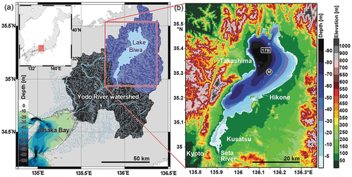
Figure 1. (a) Map of the area around Lake Biwa showing the watersheds and river paths. The blue shaded area indicates the watershed flowing into Lake Biwa in the Yodo River Basin (black shaded area) flowing into Osaka Bay (colour scale indicates depth in metres). The red square denotes the study area. (b) Topography and bathymetry of the area around Lake Biwa. The black square (17B) indicates the regular monitoring site (Imazu-oki-chuo) of the Lake Biwa Environmental Research Institute (LBERI). The black dot (M) indicates the Adogawa Offshore Comprehensive Automatic Observation Station of the Japan Water Agency (JWA).

Mixing in several lakes worldwide will be less frequent and its regimes altered in response to future climate change (Shatwell et al. 2019, Woolway and Merchant 2019). Studies identifying mixing regime shifts in lakes are important as they broaden our understanding of the ongoing climate change. Ficker et al. (2017) suggested that the mixing patterns of some deep alpine lakes (Irrsee, Mondsee, and Hallstätter See) in the Salzkammergut Lake District (Austria) would be transformed from dimictic to monomictic mixing regimes under the current trend of global warming. Similarly, Valerio et al. (2015) concluded that the predicted rise in water temperature in Lake Iseo (Italy) under future climate change scenarios would reinforce thermal stability in the winter and suppress overturn, which may determine the oxygenation levels of the deep water. The period of summertime surface warming is also projected to increase in the future, which would lead to profound disturbances in the ecosystems of Lake Baikal (Piccolroaz and Toffolon 2018) and Lake Superior (Matsumoto et al. 2019). Climate-induced changes to the mixing regime in Lake Zurich would expand the hypoxic zone, which may increase the vulnerability of the ecosystem to predicted global warming (North et al. 2014). Similar mixing regime vulnerability may also be emerging in Lake Biwa (Yoshimizu et al. 2010). A pioneering study is required to develop indices for the measurement of alterations in lake mixing regimes using thermal structures (stratification and overturn) combined with climate factors, which will enable worldwide monitoring and analysis.

A lake heat budget is a useful concept that can aid in understanding the mixing regimes across various time scales (Xing et al. 2012). Heat storage, calculated using the water temperature in deep lakes, is a promising candidate indicator for monitoring the ongoing impacts of climate change, such as glacier melting and rising sea levels (Ambrosetti and Barbanti 1999). Various approaches have been proposed for the analysis of thermal structures, including a hydrological model in Lake Tahoe (Sahoo et al. 2013), a mathematical model in Mar Menor coastal lagoon (southeast Spain) (Martínez-Alvarez et al. 2011), and an empirical procedure applied to 22 lakes (Duan and Bastiaanssen 2015). In Lake Ikeda, a one-dimensional heat transfer model based on a heat budget successfully reproduced the characteristics of the thermal structures (Momii and Ito 2008). Thus, the analysis of heat budgets in deep lakes is common, since the surface heat flux (heating and cooling) develops into thermal stratification and overturn (Sahoo et al. 2013). The evaluation of surface heat flux and heat storage in a water column is also essential to estimate the onset of stratification and overturn, in addition to the heat budget (Lewis and William 1983, Talling 2001). Based on these studies, a heat budget analysis focusing on the interruption of monomictic mixing in Lake Biwa could provide a valuable assessment of mixing regime shifts in lakes.

Several studies have utilized the thermal structure of Lake Biwa to investigate model reproducibility (Akitomo et al. 2009b, Koue et al. 2018a), meteorological sensitivity of thermal stratification (Koue et al. 2018b, 2018c), and gyre generation (Akitomo et al. 2004, 2009a). However, no previous studies have focused on mixing regime shifts relative to surface heat fluxes based on a heat budget analysis. Previous modelling studies have aimed to reproduce and/or predict thermal stratification (Kitazawa et al. 2018, Koue et al. 2018a) and water quality (Kitazawa et al. 2010, 2018, Kitazawa 2011) associated with ecosystems (Sato et al. 2011) in response to secular increases in air/water temperature under climate change scenarios (Yoshida et al. 2018). However, the factors that dominate the observed interruptions or underlie the retardation of monomictic mixing in 2018/2019 in Lake Biwa remain unknown.

Although lake surface winds dominate the magnitude of convective overturn through the processes of vertical momentum mixing and surface cooling, the air/water temperature and surface moisture on the lake also affect overturn. Woolway et al. (2017) found that previous studies typically only considered the responses of a lake to rising air temperature. However, more recent studies have focused on the alterations in the vertical mixing due to wind speed changes, which are observed in addition to rising air temperatures (Desai et al. 2009, Magee and Wu 2017, Wang et al. 2021). The mixed layer depth may change to a greater extent due to spatiotemporal variations in water transparency or wind speed (Shatwell et al. 2019). For example, atmospheric stilling (decreasing wind speeds) in Lake Võrtsjärv has resulted in a substantial change in the stratification dynamics, whereas increasing air temperatures during the same period had a negligible effect (Woolway et al. 2017). The increasing surface wind speeds over Lake Baikal enhanced deep ventilation, leading to dramatic increases in nutrient supply from deep waters to the photic zone (Swann et al. 2020). Simulation results of Yoshida et al. (2018) and Koue et al. (2018c) suggested that surface winds determined the magnitude of monomictic mixing and summertime stratification in Lake Biwa. Although these research outcomes have been accumulated, available information for evaluating mixing regime shifts is still limited in many deep lakes due to a lack of in situ data on meteorological properties (e.g. air temperature, humidity, wind) and limnological profiles (e.g. water temperature, flow field). With respect to Lake Biwa, this research gap should be rectified by investigating the relationships between the observed interruption of monomictic mixing and changes in various meteorological factors using a numerical simulation to reproduce the limnological profiles.

The present study aimed to identify the factors which can affect monomictic mixing interruption in Lake Biwa. To this end, a heat budget analysis was conducted focusing on the surface cooling from autumn to the following spring using a realistic, three-dimensional lake circulation model. The surface cooling inducing the overturn in Lake Biwa was evaluated as a function of meteorological conditions, such as air/water temperature, humidity, and wind speed. Furthermore, the study presents an appropriate index to detect inter-annual alterations in warm-monomictic mixing.

2 Materials and methods

2.1 Study area

With a volume of 27.5 km³, Lake Biwa is the largest lake in Japan. It is located on the central island of the Japanese archipelago, Honshu (Fig. 1). The lake has a surface area of 670 km² and provides water for human consumption, irrigation, and industrial use to approximately 14.5 million people in Shiga, Kyoto, Osaka, and Hyogo prefectures. Lake Biwa consists of two basins, a deep north basin (mean depth 41 m, maximum depth approximately 104 m) and a shallow south basin (mean depth 4 m) (Haga et al. 2007). The climatological water surface altitude of the lake is approximately 85 m (Ikebuchi et al. 1988) above the low tide level in Osaka Bay (Fig. 1).

2.2 Data acquisition

The hydrographic observations and bottom topography of the lake are shown in Fig. 1. Observational temperature data were obtained from LBERI from September 2017 to March 2019. LBERI made regular observations, which were compiled from the research vessel (R/V) Biwa-kaze, by casting a multi-probe water quality sonde (Hydrolab DS5, Hach Company, Loveland, CO, USA) at a fixed station (17B) in Lake Biwa (Fig. 1). Water temperature data were derived for 12 depths (0.5, 5, 10, 15, 20, 30, 40, 60, 70, 80, 85, and 88 m) and used to validate the simulated water temperatures. All observed water temperature data were provided after a quality check in which abnormal and error values were removed.

The input data used for the simulation were obtained from the Grid Point Value datasets of the Meso-Scale Model (GPV-MSM) prediction dataset (Koreeda et al. 2003). The meteorological data used in this study were air temperature, dew point temperature, and wind speed (http://www.jmbsc.or.jp/jp/index.html). They were compared with the observed meteorological data provided by the Japan Water Agency (JWA) to verify the input data during the analysis period. The meteorological measurement data were recorded at the Adogawa Offshore Comprehensive Automatic Observation Station (Fig. 1) operated by the JWA (https://www.water.go.jp/kansai/biwako/html/report/report_02.html).

2.3 Lake circulation model

A numerical simulation was performed using the Research Institute for Applied Mechanics Ocean Model (RIAMOM) with realistic bottom topography and a horizontal grid resolution of approximately 500 m for both longitude and latitude. RIAMOM is a three-dimensional ocean circulation model with hydrostatic and Boussinesq approximations (Lee et al. 2003, Hirose et al. 2007) that has successfully simulated regional flow fields in previous studies (e.g. Kawamura et al. 2007, Sasajima et al. 2007, Moon et al. 2009, Nakada et al. 2010, 2014, Hirose 2011, Hirose et al. 2017, Jeon et al. 2019). It solves free-surface primitive equations and implements a momentum advection scheme that allows slant advection at the lateral boundary (Ishizaki and Motoi 1999). The vertical grid intervals begin from 2 m around the surface, except for the first layer (3 m thickness), and extend to 5 m around the bottom, as shown in Table 1. The model used in the present study was composed of a time-splitting system (Mellor 1998), and the time steps in the external and internal modes were 0.5 and 10 seconds, respectively. The 50 m meshed bathymetry dataset (Fig. 1(b)) distributed by LBERI was used, and the bathymetry data were blended into the model grids using Gaussian-type weighted interpolation.

Table 1. Thickness and centre depth of layer at each level used in the model.

Layer #	Thickness (m)	Centre depth of layer (m)
1	3	1.5
2	2	4.0
3	2	6.0
4	2	8.0
5	2	10.0
6	2	12.0
7	2	14.0
8	2	16.0
9	2	18.0
10	2	20.0
11	3	22.5
12	3	25.5
13	3	28.5
14	4	32.0
15	4	36.0
16	4	40.0
17	4	44.0
18	4	48.0
19	4	52.0
20	4	56.0
21	4	60.0
22	4	64.0
23	4	68.0
24	4	72.0
25	5	76.5
26	5	81.5
27	5	86.5
28	5	91.5
29	5	96.5
30	5	101.5

Isopycnal and thickness operators (Gent and Mcwilliams 1990) to evaluate the lateral eddy diffusivity were adopted in our model instead of the conventional Cartesian horizontal diffusion similarly (e.g. Hirose et al. 2007). Details regarding the isopycnal mixing scheme can be found in the study by Kim and Yoon (1999). The horizontal eddy viscosity was calculated using a combination of harmonic and biharmonic operators with constant coefficients of 0.5 m² s^–1 and 1.0 × 10⁸ m⁴ s^–1, respectively. Those constant coefficients were determined by trial and error to reproduce the observed water temperatures, referring to the values used by Hirose (2011). The biharmonic operator can allow eddy permitting simulations and scale selectivity of the dissipation, and more strongly selects the small scales to dissipate, leaving the large scales relatively untouched. The vertical viscosity and diffusion coefficients were assumed to be constant at 1.0 × 10⁻⁶ and 1.0 × 10⁻⁶ m² s^–1, respectively. The coefficients were used as the background in our model under the usage of the isopycnal and thickness operators. Such an assumption was often adopted for realistic flow simulations in previous studies (e.g. Hirose 2011). Although their viscosity might be close to the kinematic viscosity coefficient, similar values have also been used in some numerical flow simulations (e.g. Garvine 1999, Li et al. 2005). Kumagai et al. (1986) reported that the vertical diffusion profile estimated from the observational data in Lake Biwa also suggested a small value close to the kinematic viscosity. Therefore, the coefficients were determined by trial and error to improve the reproducibility of the simulated water temperatures and to satisfy the numerical stability within the ranges of values used in previous studies (Kumagai et al. 1986, Akitomo et al. 2004, 2009b, Hirose 2011).

The initial water temperature or thermal stratification conditions were provided as horizontally homogeneous temperature profiles using the temperature data collected from the R/V Biwa-kaze of LBERI in late August 2017 and 2018. Time integration was performed for 210 days from an initial state of rest on 1 September.

The RIAMOM relies on the GPV-MSM provided by the Japan Meteorological Agency (JMA) for the required high-resolution meteorological surface forcing conditions used in the present simulation, rather than observations (e.g. satellite-measured winds, QuikSCAT with coarse spatial resolution, ~25 km). The forcing dataset contains mean hourly data on four meteorological variables: air temperature 2 m above the water (T_a; °C), cloud cover (Cl), relative humidity 2 m above water (Rh), and surface wind speed at 10 m above water (W; m s⁻¹). The GPV-MSM data, with horizontal resolutions of 0.05° × 0.0625° on the ground and lake, were interpolated onto the model grids based on the spline method (Nakada et al. 2012). The predictive accuracies of T_a, Rh, and W were verified, and the regional representativeness and predictabilities of the interpolated T_a and Rh values were confirmed, as shown in Appendix A (Fig. A1). However, a scaling factor (approximately 1.6) for the interpolated W values was applied to the wind speeds used to reproduce realistic water temperatures since that of the GPV-MSM may have low predictability on the lake (Fig. A2). Piccolroaz et al. (2019) and Woolway et al. (2017) also found a close or comparable scaling factor, implying an underestimation of the lake surface wind using simulated wind or observed land surface wind. Similar results were obtained by Nakada et al. (2021). The momentum fluxes (${\tau }_x$, ${\tau }_y$) for the RIAMOM were computed from W using the bulk formulation as (${\tau }_x$, ${\tau }_y$) = ${\rho }_a{C}_{D}W(w_x$, $w_y)$ (Gill 1982), where $w_x$ and $w_y$ are the x and y components, respectively, of the wind vector, W =${\left({w_x}^2+{w_y}^2\right)}^{1/2}$, ${\rho }_a$ is the air density, and $C_D$ is the drag coefficient with a function of W (Kondo 1975). For the heat fluxes, the shortwave and longwave radiative fluxes and the latent and sensible heat fluxes were directly computed using T_a, Rh, Cl, and W with simulated lake surface temperatures, T_s, based on the Kondo (1975) bulk formula. The detailed heat flux calculations are explained in the next subsection.

2.4 Heat analytical method

The surface heat fluxes were calculated using the GPV-MSM data and radiation balance, based on the formulae outlined by Hirose et al. (1996). The net heat input at the surface of each grid of the numerical domain $Qn$ can be written as

(1) $\mathrm{Q}\mathrm{n}=\mathrm{S}+\mathrm{L}+\mathrm{H}+\mathrm{I}\mathrm{E}$(1)

(2) $S=I_0\left(1-a_{1}Cl\right)\left(1-{\alpha }_s\right)$(2)

(3) $L=\epsilon \sigma {\theta }_a^4\left(a_2-a_3{e}_a\right)\left(1-\delta Cl\right)+4\epsilon \sigma {\theta }_a^3\left(T_s-T_a\right)$(3)

(4) $H=c_p{\rho }_a{C}_{H}W\left(T_a-T_s\right)$(4)

(5) $IE=l{\rho }_a{C}_{E}W\left(q_a-q_s\right)$(5)

where $S$, $L$, $H$, and $IE$ represent the incoming solar radiation, net longwave radiation, sensible heat flux, and latent heat flux, respectively. The calculations used for the four surface fluxes are similar to those used in previous modelling studies at Lake Biwa (Akitomo et al. 2009b, Koue et al. 2018a) and were derived from GPV-MSM using the pre-analysis meteorological dataset ($T_a$, Cl, Rh, and W) in this study. In addition, $I_0$ represents the solar radiation under a clear sky (Reed 1977); ${\alpha }_s$ (= 0.06) represents the albedo at the lake surface (Momii and Ito 2008); $e_a$ is the actual vapor pressure; $\epsilon$ is the emissivity at the lake surface (= 0.97); $\sigma$ is the Stefan-Boltzmann constant; ${\theta }_a$ is the air temperature in K; the values of $a_1$ (= 0.62), $a_2$ (= 0.254), and $a_3$ (= 0.00495) are constants; ${\rho }_a$ is the air density; $c_p$ represents the specific heat of the air at constant pressure; l is the latent heat of evaporation; $q_s$ is the saturated specific humidity at the lake surface temperature, $T_s$; and $q_a$ is the actual specific humidity. In Equation (3)(3) $L=\epsilon \sigma {\theta }_a^4\left(a_2-a_3{e}_a\right)\left(1-\delta Cl\right)+4\epsilon \sigma {\theta }_a^3\left(T_s-T_a\right)$(3) , $\delta$ represents the cloud coefficient, which is a function of latitude and ${\theta }_a$, and is used instead of water temperature for Stefan-Boltzmann’s law following the formulae proposed by Hirose et al. (1996). The direct heat transport by precipitation was assumed to be small and negligible. The detailed calculations used to derive $I_0$, $q_s$, $q_a$, and $e_a$ using $T_a$, p, Cl, and Rh are described by Kondo (1975) and Kondo and Watanabe (1992) as approximate formulae for diabatic conditions.

The heat budget analysis at the lake surface was based on the following calculations (Nakada et al. 2013). The integration of the net surface flux ($QN$) and heat storage ($HS$) over the entire lake can be calculated using the following equations:

(6) $QN=\underset{A}{\int \int }Qndxdy$(6)

(7) $HS=\underset{V}{\int \int \int }Hqdxdydz$(7)

where $A$ is the total area of the lake as distinguished by the boundary line along the lake mouth (Fig. 1), and $V$ is the total volume of lake water. The $x$, $y$, and $z$ spatial variables take the eastward, northward, and upward directions, respectively, as positive values. The heat storage in each grid $Hq\left(=C_p{\rho }_w{T}_w\right)$ was calculated using the specific heat $C_p\left(=4.18\mathrm{k}\mathrm{J}\cdot {\mathrm{K}}^{-1}\right.$ $\left.\cdot \mathrm{k}{\mathrm{g}}^{-1}\right)$, freshwater density ${\rho }_w$, and lake water temperature $T_w$ at an arbitrary level.

The lake mixing index ($LaMIX$) of the present year was defined as the heat storage ($HS$) normalized by the minimum total heat storage $H{S}_{min\left(PY\right)}$ of the previous year in which monomictic mixing occurred, which can be calculated using the following equation:

(8) $LaMIX=HS/H{S}_{min\left(PY\right)}$(8)

where $PY$ indicates the previous year. In this study, the period of analysis was defined as the cooling season from September to March, and the previous year (PY) was defined as the period from 1 April to 31 March. Therefore, the cooling season in 2017/2018 (2018/2019) was defined as the period from September 2017 (2018) to March 2018 (2019). The preliminary simulation was conducted for the period from 1 September 2016 to 31 March 2017 to estimate the minimum total heat storage $H{S}_{min\left(2016/2017\right)}$ in advance (not shown).

2.5 Statistical spatial analysis of mixed layer depth

The total area when the full overturn was completed ($A_{FO})$ and the total volume retaining the mixed layer (overturn depth, $V_{ML})$ were estimated in the entire lake as defined by the following equations:

(9) $A_{FO}=\hspace{0.17em}\underset{\mathrm{A}}{\int \int }{\delta }_{MLD}dxdy$(9)

(10) $where,{\delta }_{MLD}=\left\{\begin{array}{c}1MLD=h\left(x,y\right)\\ 0MLD<h\left(x,y\right)\end{array}\right.$(10)

(11) $V_{ML}=\underset{\mathrm{A}}{\int \int }MLD\left(x,y\right)\hspace{0.17em}dxdy$(11)

where $h\left(x,y\right)$ is the bathymetry depth in Lake Biwa, and $MLD\left(x,y\right)$ represents the mixed layer depth. $MLD$ is defined by the depth from the surface to an arbitrary level under the condition of the vertical water temperature differences, $\mathrm{\Delta }T$ (=$T_s-T_w$) < 0.5°C (Obata et al. 1996). In Equation (10), ${\delta }_{MLD}=1$ means that the full overturn has occurred when $MLD$ reaches the lake bottom, $h$. Then, we counted the number of days ($D_{FO}$) that the full overturn occurred in each computational grid.

2.6 Sensitivity experiment

We conducted a sensitivity experiment to qualitatively understand how meteorological factors, such as air temperature rise and change in lake surface wind speed, affect the strength of the full overturn in Lake Biwa. The 12 total perturbation cases (Table 2) were evaluated by increasing the air temperature ($T_a$) by 1–3°C and changing the lake surface wind speed ($W$) from −30% (reduction) up to +30% (gain). All physical parameters of the model were the same for all experiments in 2017/2018 and 2018/2019. The default case with no increase in the air temperature and no change in the wind speed during both years is the control run (CR) for the sensitivity experiment. The number of days ($D_{FO}$) when the full overturn occurred was counted in each sensitivity analysis.

Table 2. Sensitivity experiment for 12 cases in 2017/2018 and 2018/2019 with different perturbed values for the air temperature and wind speed with respect to sensible and latent heat fluxes.

Year	Property	Experimental case names
2017/2018	Air temperature
	Increases 1°C	Ta + 1°C
	Increases 2°C	Ta + 2°C
	Increases 3°C	Ta + 3°C
	Wind speed
	Decreases 10%	W – 10%
	Decreases 20%	W – 20%
	Decreases 30%	W – 30%
2018/2019	Air temperature
	Increases 1°C	Ta + 1°C
	Increases 2°C	Ta + 2°C
	Increases 3°C	Ta + 3°C
	Wind speed
	Increases 10%	W + 10%
	Increases 20%	W + 20%
	Increases 30%	W + 30%

3 Results

3.1 Simulation accuracy

The quantitative reproducibility of the simulation used in the present study can be verified objectively using numerical indices representing the accuracy of the simulation. A scatter plot of the simulated and observed temperatures used to quantitatively validate the simulated results is presented in Fig. 2 and indicates a strong positive correlation for the analysis period (R² = 0.95, n = 336, p < .01). The anomaly correlation coefficient (AC), an index representing model accuracy (Smedstad et al. 2003), is estimated using the following equation:

(12) $AC\left(f,x\right)=\sum (f-\overline{f})\left(x-\overline{x}\right)/\sum {\left(f-\overline{f}\right)}^2\sum {\left(x-\overline{x}\right)}^2$(12)

(for detailed terminology see Murphy and Epstein 1989), where $f$ and $x$ represent the simulated and observed water temperatures, respectively; and $\bar{f}$ and $\bar{x}$ are the climatologically averaged simulated and observed water temperature values, respectively. The high AC values (AC = 0.97) obtained indicated that the reproducibility of the simulation was also satisfactory. AC values >0.6 are considered to indicate a practical prediction ability (Smedstad et al. 2003). The root mean square error (RMSE), bias, and mean absolute error (MAE = $\overline{\left|f-x\right|}$) of the water temperatures were calculated (bias, −0.05°C; RMSE, 1.16°C; MAE, 0.57°C) to evaluate the accuracy of the simulated water temperature compared to the observed water temperature and indicated sufficient accuracy of the analyses (a detailed evaluation is presented in the Discussion).

Figure 2. Scatter plot showing the simulated and observed water temperatures at 17B, the fixed station (Fig. 1), during the cooling period in 2017/2018 and 2018/2019.

The skill score (SS) (Murphy and Epstein 1989) is used to validate the predictive ability of a model and is defined as

(13) $SS\left(f,x\right)=1-\sum {\left(f-x\right)}^2/\sum {\left(x-\overline{x}\right)}^2$(13)

, with SS values <0.5 implying an unsatisfactory practical prediction ability (e.g. Moriasi et al. 2007). The SS result for the simulation used in the present study (SS = 0.93) indicates the usefulness of the model (Murphy and Epstein 1989). This suggests that the model simulated the water temperature associated with vertical mixing in the cooling season.

The vertical profiles of the simulated water temperatures were additionally compared with the in situ temperatures at the observation station (17B) to validate the model reproducibility in detail using the RMSE (see Appendix B). The RMSE in the deeper layer (>60 m depth) was within 0.5°C, corresponding to the mixed layer depth (MLD) definition (Obata et al. 1996). To satisfy this threshold, referred to as the calculation accuracy of the water temperature, the model was calibrated with trial and error. This is because we focused on a heat storage analysis associated with MLD formation in the overturn season, winter. Therefore, the above metrics also show that the simulation produced satisfactory values for robust analyses, as verified by the observational data.

3.2 Overturn in 2017/2018 and 2018/2019

The simulated water temperatures were compared with the in situ temperatures observed at 17B, the regular monitoring station (Fig. 1), which was located at the deepest section of the north lake at a depth of 88 m. The study focused on the typical temperature stratification and a vertical mixed layer, which were the benchmarks used to validate the simulated results. Hovmöller (time-depth) diagrams of the simulated and observed water temperatures in 2017/2018 and 2018/2019 during the cooling period from September to March are presented in Fig. 3. The vertical distributions of the simulated temperatures were close to those of the observed temperatures in both years, indicating that there was qualitative reproducibility of the typical vertical mixing. For example, the temporal variations in the simulated water temperatures showed that the thermocline deepened, and the mixed layer developed during the cooling period. This suggests that vertical mixing or overturn began in September each year and deepened the mixed layer depth located above the thermocline.

Figure 3. Hovmöller diagrams of the hourly vertical profiles of the simulated water temperatures (colour shades) during the cooling period from September to March in (a) 2017/2018 and (b) 2018/2019, and observed water temperatures (17B in Fig. 1) denoted by the coloured dots. White dots indicate the daily mean mixed layer depth (bottom of the mixed layer). Black column-like contours around mid-October in 2017 indicate the dense isotherms.

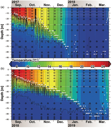
Inter-annual differences in water temperature were clearly observed between 2017/2018 and 2018/2019 based on the simulated and observed data. Thermal stratification was observed in September of both years. The main thermocline in 2017/2018 deepened rapidly with strong vertical fluctuations, whereas in 2018/2019, the thermocline deepened smoothly from September to March. The mixed layer depth increased by 0.26 m s⁻¹ from September 2017 before the category 4 super-typhoon (Lan) hit on 23 October and vertically mixed, as shown by black column-like contours; and the depth after Typhoon 21 increased even more rapidly, by 0.74 m s⁻¹, until January 2018. Thermal stratification was hardly present from January to March 2018, suggesting that there was a strong overturn at all depths of the water column. In contrast, the speed at which the mixed layer deepened in 2018/2019 was 0.35 m s⁻¹ slower than in 2017/2018. The thermal stratification remained stable from January to March 2019, and the mixed layer depth hardly reached the bottom, indicating that vertical mixing was more dominant in 2017/2018 than in 2018/2019 and that the vertical water exchange in the water column caused by full overturning was weak in 2018/2019.

Thus, the present model successfully simulated the early start (late January 2018) of the full overturn in 2017/2018 as a typical phenomenon in Lake Biwa in winter, but the full overturn was incomplete in 2018/2019. The temporal variations in the thermoclines and mixed layer depths exhibited different features (i.e. simulated patterns and tendencies of temperature profiles) between the years. These simulation results illustrate the inter-annual differences in the full overturn between the studied years.

3.3 Simulated gyres

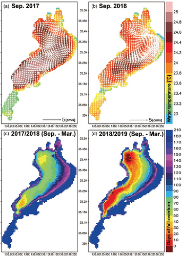
The simulated flows in 2017/2018 and 2018/2019 were compared with the typical lake circulations shown in previous studies for qualitative validation (Suda 1926, Endoh and Okumura 1993) because no data on current observations were available to compare. As an example of the typical circulations, Fig. 3(a) and (b) shows two large summertime gyres, referred to as the first and second gyres (Suda 1926), which were qualitatively simulated in the northern part of the lake in September 2017 and 2018. The first gyre was the largest and circulated counterclockwise, and its centre was generally located between 35.3 and 35.35°N. The second gyre circulated clockwise, and its centre in 2017 was located around 35.25°N. These typical circulations formed in the summer and were previously reported by field observations based on the trajectories of the drifters and current measurements of the surface layer (e.g. Endoh and Okumura 1993). However, the second gyre in 2018 was less well defined because of the category 5 super typhoon 21 (Jebi) that hit Lake Biwa on 4 September 2018 and generated a high-speed flow. The simulated water temperatures in the northern and southern parts of the lake in 2017 were largely higher (>24.4°C) and lower (<23.2°C), respectively, than those in 2018, which was consistent with the observational results obtained by LBERI.

3.4 Simulated full overturn

The number of days ($D_{FO}$) during which full overturn occurred for each grid in 2017/2018 and 2018/2019 is identified in Fig. 4(c) and (d), respectively. The number of days of full overturn exceeded 10 days in all grid spaces in 2017/2018, indicating that monomictic mixing (seasonal full overturn) occurred to completion. In contrast, in 2018/2019, there were areas with zero days of full overturn, and large areas with fewer than 10 days (red areas) of full overturn in the western part of the lake, indicating that the full overturn was incomplete – the areas with <10 days corresponded to those with deep bathymetry (<−70 m). The simulation results were in agreement with the observed fact that monomictic mixing did not occur in 2018/2019 in Lake Biwa.

Figure 4. Maps of the monthly-mean simulated water temperature (colours) and velocity fields (vectors) in the surface layer at 4 m depth in (a) September 2017 and (b) September 2018, and the occurrence in days of simulated full overturn during the cooling period from September to the following March in (c) 2017/2018 and (d) 2018/2019.

3.5 Heat budget analysis

To identify the physical factors involved in the weaker overturn in 2018/2019, we evaluated the heat storage (HS) using the simulated results and the vertical heat transport through the lake surface based on Equations (1(1) $\mathrm{Q}\mathrm{n}=\mathrm{S}+\mathrm{L}+\mathrm{H}+\mathrm{I}\mathrm{E}$(1) –5(5) $IE=l{\rho }_a{C}_{E}W\left(q_a-q_s\right)$(5) ), and their temporal variations were compared with the variations in the overturn strength (Fig. 5).

Figure 5. Heat budget and overturn analyses of Lake Biwa during the cooling periods in 2017/2018 (left panels) and 2018/2019 (right panels). Temporal variations in the 25 h running mean (upper panels) of the spatial occupancy of the overturn; total percentage areas of the simulated full overturn (A_FO) per entire lake area (670 km²) and the volume of the mixed layer (V_ML) per entire lake volume (27.5 km²). Middle panels: the surface heat flux areas are averaged over the whole lake; incoming solar radiation (S); net longwave radiation (L); sensible heat flux (H); latent heat flux (IE). Lower panels: the heat flux and heat storage of the lake; Bowen ratio (Br), net surface heat flux (QN), and heat storage (HS) corresponding to the mixing index (LaMIX) scaled by the vertical axis located between the panels. Lateral red lines indicate HS = 1000 in petajoules (PJ). White lines indicate LaMIX = 1 each year, indicating the monomictic mixing regime in the lake.

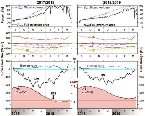
The upper panels in Fig. 5 show that the area of the simulated full overturn and the volume of the mixed layer gradually increased from smaller values (<40%) in September each year. The area was close to 100% at the end of January in 2017/2018, but in 2018/2019, it was only 50–70%. The volume from mid-January to mid-March exceeded 90% in 2017/2018. A continuous period during which the area and volume both reached 100% was visible three times in 2017/2018, indicating that monomictic mixing occurred in Lake Biwa. In contrast, the volume in 2018/2019 fell to 90–100% from mid-February to mid-March, and the area did not reach 100%, indicating that monomictic mixing in 2018/2019 was weak or partially absent.

The middle panels in Fig. 5 represent each component of the surface fluxes, indicating that the temporal variations in longwave radiation flux (L), sensible heat flux (H), and latent heat flux (IE) were mostly negative, apart from the solar insolation (S). The magnitude of IE was the smallest of the three fluxes in both years, and L and H were the second and/or third smallest, respectively. The temporal variations in these components were similar to those found in previous studies (Akitomo et al. 2009b; Koue et al. 2018).

Negative values were largely obtained for the temporal variation in QN in both years (lower panels in Fig. 5) calculated using Equation (6), although components of S, L, H, and IE exhibited down–up temporal variations. The temporal variations in QN and HS show that negative QN values gradually reduced HS, indicating seasonal surface cooling. Two zero-crossing points of the QN observed in September and March corresponded to the start and end of the cooling period, respectively. The minimum QN occurred around December in both years. The temporal variations in HS were strongly correlated with those in IE. Furthermore, IE was always negative, and the Bowen ratio (=H/IE) ranged from −0.1 to 0.5 in both years, indicating that IE was more than two-fold greater than H. This explains why IE had a major impact on surface cooling, and the temporal variation in IE can be determined by the variation in HS during the cooling period.

The temporal variations in QN in 2017/2018 followed a different pattern to those in 2018/2019, since the QN in 2017/2018 decreased to a larger extent in the period from November to December, although the temporal fluctuations in the QN were similarly visible in both years. The increase in QN from January was milder in 2019 than in 2018. When LBERI confirmed that there was a full overturn in the entire lake (monomictic mixing) on 22 January 2018, the temporal variation in the lake mixing index, LaMIX, in 2017/2018 decreased to just below 1 (approximately 1000 × 10¹⁵ PJ) and underran from January to March in 2018. In contrast, the temporal variation in LaMIX in 2018/2019 never fell below 1 (HS > approximately 1000 PJ). The LaMIX of 2018/2019 was larger than that of 2017/2018 due to the lower water temperature in March 2017. Therefore, the mixing pattern in Lake Biwa in both years was accurately represented by the mixing index, LaMIX, which was calculated using heat storage.

3.6 Inter-annual differences in the heat budget

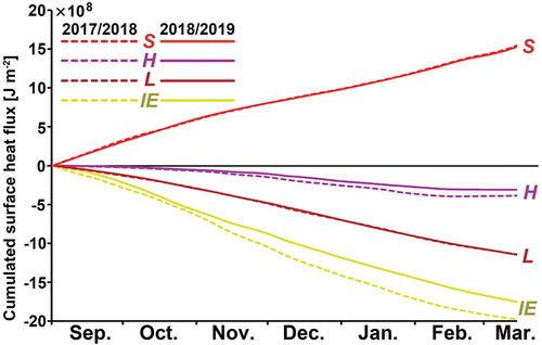
The cumulative surface heat fluxes of S, H, L, and IE were calculated (Fig. 6) during the period from September to March in both years to evaluate the inter-annual differences in those components. The temporal variations in the cumulative S and L showed increases and decreases, respectively, in both years, indicating few inter-annual differences. In contrast, H and IE exhibited clearly different decreases between the years, indicating that H and IE in 2017/2018 were lower than those in 2018/2019. The cumulative IE was always negative, and its magnitudes at the end of March 2017/2018 and March 2018/2019 were more than 5.7- and 5.1-fold those of H, respectively. These results indicate that IE primarily contributed to the stronger surface cooling observed in 2017/2018 than in 2018/2019, whereas H was a secondary factor.

Figure 6. Time series of the cumulative surface heat flux, incoming solar radiation (S), net longwave radiation (L), sensible heat flux (H), and latent heat flux (IE) during the cooling period (September–March) in 2017/2018 (dotted lines) and 2018/2019 (solid lines).

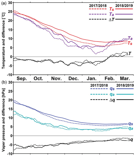
To detect the meteorological factors that primarily influenced the inter-annual differences in H and IE, we analysed the inter-annual differences in six meteorological variables and their daily means, including air and water temperatures (T_a and T_s) and their differences (ΔT = T_a − T_s), and the actual and saturated vapor pressures (q_a and q_s) and their differences (Δq = q_a − q_s) in both years, using Equations (4)(4) $H=c_p{\rho }_a{C}_{H}W\left(T_a-T_s\right)$(4) and (5(5) $IE=l{\rho }_a{C}_{E}W\left(q_a-q_s\right)$(5) ). Figure 7 shows the temporal variations in the six meteorological components, indicating that T_a and T_s in 2017/2018 were largely lower than those in 2018/2019. Notably, the temperature differences (ΔT) did not differ greatly between the years, and the time-averaged ΔT was within 0.3°C (Table 2). The temporal variations in q_s and q_a were predominantly lower in 2017/2018 than in 2018/2019; meanwhile, Δq was higher in 2017/2018 than in 2018/2019, but the time-averaged Δq values were within 0.3 (Table 2).

Figure 7. Time series of the 25 h running mean of (a) air temperature (T_a), surface water temperature (T_S), and their differences (∆T = T_a − T_s) to evaluate the contribution of temperature to H in Equation (4)(4) $H=c_p{\rho }_a{C}_{H}W\left(T_a-T_s\right)$(4) ; and (b) specific humidity (q_a), saturated specific humidity (q_S), and their difference (∆q = q_a − q_s) to evaluate the contribution of humidity to IE in Equation (5)(5) $IE=l{\rho }_a{C}_{E}W\left(q_a-q_s\right)$(5) during the cooling period (September–March) in 2017/2018 (dotted lines) and 2018/2019 (solid lines). All properties used for the time series were area averaged across the whole lake.

The temporal variations in daily mean wind speed (W) in both years and their differences (ΔW: 2017 values minus 2018 values) are shown in Fig. 8, and wind speed was generally found to be stronger in 2017/2018 than in 2018/2019. In particular, the differences in wind speed ΔW were large, reaching approximately 4 m s⁻¹ in the period from October to January. Table 3 shows that the inter-annual difference in the area- and time-averaged wind speed (ΔW) was approximately 1.3 m s⁻¹. These results imply that wind in the cooling period was the most dominant factor affecting surface cooling throughout the year.

Figure 8. Time series of the 25 h running mean for wind speed (W) during the cooling period (September–March) in 2017/2018 (dotted lines) and 2018/2019 (solid lines); the differences (∆W) between W in 2017/2018 minus W in 2018/2019 were used to evaluate the differences in the magnitudes of H and IE. All properties used for the time series were area averaged across the whole lake.

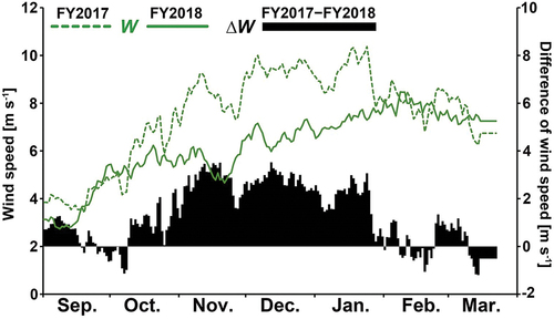
Table 3. Time-averaged values of the meteorological factors during the cooling period from September to the following March in 2017/2018 and 2018/2019, and the differences between years.

		2017/2018	2018/2019	Difference(2017–2018)
Temperature (°C)
Air temp.	Ta	10.6	11.8	−1.2
Water temp.	Ts	12.5	14.0	−1.5
Difference	Ta – Ts	−1.9	−2.2	0.3
Specific humidity
Actual	qa	5.5	5.9	−0.4
Saturated	qs	9.5	10.2	−0.7
Difference	qa – qs	−4.0	−4.4	0.3
Wind speed (m s^−1)
	W	7.5	6.2	1.3

3.7 Sensitivity analyses for the full-overturn occurrence

Figure 9 depicts the map of $D_{FO}$ based on the sensitivity experiment results in 2017/2018 and 2018/2019. $D_{FO}$ in 2017/2018 decreased with rising air temperature or reducing the surface wind speed, but $D_{FO}$ did not reach 0 days. For example, the range of $D_{FO}$ was $D_{FO}$ > 30 days in the CR case (Fig. 2), but decreased to $D_{FO}$ > 20 days in the T + 3°C case and $D_{FO}$ > 0 days in the W − 30% case. The range of $D_{FO}$ in the case W − 10% took $D_{FO}$ > 20 days around the lake basin, which was similar to the results in the case T + 2°C. This suggests that a 2°C rise in temperature has a similar influence to a 10% reduction in wind speed.

Figure 9. Maps of the days of full-overturn occurrence (D_FO) in each case of the sensitivity experience (Table 2) during the cooling period from September to the following March in 2017/2018 and 2018/2019.

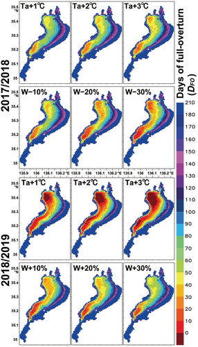
In 2018/2019, the area of $D_{FO}$= 0 days (where full overturn never occurred) was expanded owing to the air temperature rise. In particular, the area of $D_{FO}$= 0 in the case of T + 3°C was remarkably expanded in/around the lake basin. In contrast, in the cases of the wind speed changes, $D_{FO}$ increased along with the wind speed gain. In the case of W + 10%, the area of $D_{FO}$ = 0 seen in CR of 2018/2019 disappeared. This suggests that if the wind speed was approximately 10% higher in 2018, full overturn could have occurred throughout Lake Biwa.

4 Discussion

The simulation used in the present study for Lake Biwa effectively reproduced the partially incomplete full overturn or interruption of monomictic mixing in the winter of 2018/2019. This alteration in the mixing pattern was identified by the simulated full overturns and the index (LaMIX) based on heat storage. Yamada et al. (2021) indicated the first event of an incomplete vertical circulation in 2018/2019 since the monitoring of Lake Biwa started in 1979. These results suggest that the current monomictic lake may transform into an oligomictic lake where turnover might occur every few years if the wind speed decreases with future climate change. Similar shifts in the mixing regime have been observed in local lakes due to decreasing wind speeds (Magee and Wu 2017). Our results are highly complementary to recent studies that have identified the influence of atmospheric stilling on lake stratification and mixing (Stetler et al. 2021). The mixing pattern can be considered an indicator of climate change as well as deep-water warming in lakes (Ambrosetti and Barbanti 1999).

This pilot study highlighted that the alteration in the mixing pattern in Lake Biwa was primarily due to reduced wind speeds, particularly during the cooling season from autumn (October) to the following winter (January). Previous numerical studies have suggested that surface wind can determine the magnitude of the overturn (Koue et al. 2018c, Yoshida et al. 2018). Moreover, the heat budget analysis in the present study demonstrated that lower surface wind speeds could lead to weak surface cooling and weak overturn. This supports the findings of previous studies that ongoing decreases in wind speed, rather than rising air temperatures, elongate the period of thermal stratification in various lakes (Woolway et al. 2017). The analysis in the present study indicated that smaller latent and sensible fluxes decreased surface cooling in 2018/2019, which was weaker than in 2017/2018. The magnitude of the latent flux was larger than that of the sensible flux and longwave radiation flux during the cooling season, which is consistent with the normal Bowen ratio (<0.6) in Lake Biwa (Ito 1960, Arai 1962). Throughout the cooling season in deep lakes, wind speed is the most dominant factor involved in surface cooling, rather than air temperature or humidity, and should be considered a potential factor inducing mixing regime shifts in future investigations. The air temperature rise might secondarily contribute to weaker mixing. In summary, the interruption of monomictic mixing (alteration in the mixing regime) in Lake Biwa emerged when a breezy and warm winter (2018/2019) followed a windy and cold winter (2017/2018). This is consistent with the suggestion that other deep lakes, in addition to Lake Biwa, may be more vulnerable to monomictic mixing interruption (Yoshimizu et al. 2010).

The results of our sensitivity experiment suggested that the day of full-overturn formation is quite sensitive to the wind speed change in addition to the air temperature rise. The air temperature rise and wind speed changes assumed in sensitivity experiments may be induced by future climate change. The air temperature rise or wind speed reduction alone will not interrupt the full overturn, as shown in the sensitivity experiments of 2017/2018. However, the air temperature rise and wind speed reduction will be induced frequently at the same time by climate change. If they occur at the same time, the monomictic regime may be interrupted, as in 2018/2019, or the total number of full-overturn days may be significantly shortened. Our sensitivity experiment showed that the monomictic mixing in 2018/2019 can be achieved by the surface wind speed being increased by approximately 10%. Notably, the interruption of the monomictic regime and the shortening of the total number of full-overturn days can be sensitive to wind speed changes as well as the air temperature rise.

The accuracy of heat budget analysis depends on the reproducibility of the simulated water temperatures. The MAE (0.57°C) between the simulated and observed water temperatures was approximately 6% of the water temperature amplitude (18.6°C) for both the observed and simulated fluctuations. The MAE is equivalent to heat storage estimation errors (66 PJ), which were within 7% of the amplitude of temporal variations in the simulated heat storage values (1011 PJ), suggesting a sufficient reproducibility of the heat storage budget analysis of the seasonal fluctuations. The errors should be insensitive to the heat budget analysis and LaMIX, although the reproducibility of the thermal stratification range of 15–25°C in September 2018 (Figs. 3 and 4) influenced the RMSE (=1.16°C). The accuracy being affected by the model limitation could be attributed to the parameterization for the viscosity and diffusion used in the simulation. It will be necessary to establish a methodology optimizing parameters for better reproductivity of the vertical profiles of water temperature in future studies.

The simulation used in the present study reproduced the observed water temperatures during the cooling period, although the heat influx and efflux through all rivers and submerged groundwater discharges were overlooked from the simulation. Lake Biwa is fed by more than 100 inflowing rivers in its watershed (3174 km²), and the water is discharged through only one outlet (Kawanabe et al. 2012), the Seta River, in the south (Fig. 1). The water volume fluxes of the inflowing and outflowing rivers were 42.3 and 54.0 × 10⁸ m³ year⁻¹, respectively (Taniguchi et al. 2000). The heat fluxes along with inflow and outflow were calculated to be 1.68 and 2.14 W m⁻², respectively, assuming a difference in river water temperature of 2°C between the outflow and inflow. This temperature difference was estimated from the maximum horizontal difference along the coast of the summertime water temperature map (Fig. 2). The heat fluxes of the rivers are negligible compared to the magnitude of the temporal variations in the lake net surface heat flux, QN (Fig. 5), and the heat advection associated with riverine inflows and outflows is often considered a minor source of heat or is not measured (Xing et al. 2012). Since the assessment of heat transport from rivers is challenging, previous studies had not included riverine heat in their heat budget calculations (e.g. Keijman 1974, Colomer et al. 1996, Rouse et al. 2003, Binyamin et al. 2006, Momii and Ito 2008). River discharge may secondarily contribute to temporal variations in the surface heat flux of the lake in the intra-seasonal time scale of the cooling period.

Detecting mixing regime shifts contributes to a better understanding of the changes that occur in lake ecosystems worldwide and assessing the vulnerability of deep lakes to climate change. Foley et al. (2012) indicated that water temperatures increase at the surface layer (Arhonditsis et al. 2004) and at all depths (Livingstone 2003) as lakes respond directly to climate change (Komatsu et al. 2007). The volume-weighted mean temperatures of numerous lakes have also increased recently (Adrian et al. 2009). However, the physical responses of lakes to climate change are regionally variable and highly dependent on individual lake characteristics (Shatwell et al. 2019). For example, the warming rates in the deep oligomictic Lake Ikeda (Japan), deep monomictic Lake Biwa, and shallow monomictic Lake Washington (USA) were 0.033°C year⁻¹ (Ito and Momii 2015), 0.04°C year⁻¹ (Arai 2009), and 0.026°C year⁻¹ (Arhonditsis et al. 2004), respectively. Furthermore, heat storage has progressively increased in deep lakes (Ambrosetti and Barbanti 1999). Despite the finding that wind stress can be one of the most important factors driving overturn in deep lakes, the overturn response to decreased wind speed has not yet been investigated (Woolway et al. 2017). The results of the present study imply that Lake Biwa may be in a transitional period, shifting from a monomictic to an oligomictic mixing regime due to the decreasing surface wind speeds (atmospheric stilling). Such changes may result in undesirable effects such as declines in water quality and reductions in cold-water fish habitats (North et al. 2014).

This study has discovered that when the heat storage calculated using wintertime water temperature decreased to less than 1 (LaMIX < 1), the seasonal overturn could complete monomictic mixing in Lake Biwa. The index LaMIX, which was used to complement the interpretation of simulation data, had limited application to 2017/2018 and 2018/2019. The index is possibly adapted to the observational vertical profiles of lake water temperature, e.g. archived historical datasets derived in various lakes. In future studies, to reveal the projected mixing regime shifts from the past to the current stage of lakes, modification or extension of the index might be needed based on the detailed heat storage analysis. Therefore, it is important to continue collecting lake temperature profile data from various deep lakes to improve the detection of mixing regime shifts and long-term data analysis of lake temperatures over decadal periods under climate change.

There is an urgent need to predict alterations in lake mixing regimes and oxygenation of the hypolimnion in response to global warming in deep lakes such as Lake Biwa (Yoshimizu et al. 2010). Future studies should aim to predict mixing-regime shifts in deep lakes as one of the responses to climate change worldwide using projected future climate scenarios towards the management of water quality and ecosystems and adaptation strategies. The findings of the present study will aid in improving our understanding of lake responses to future events due to climate change – for example, decreasing surface wind speeds (atmospheric stilling) and increasing mean water temperatures (warm winters).

5 Conclusions

This study investigated the meteorological factors involved in the interruption of monomictic mixing (seasonal full overturn) in Lake Biwa, Japan, using a realistic, three-dimensional lake circulation model to analyse the heat budget. Focusing on the weak surface cooling from autumn to the following spring during the year in which monomictic mixing was interrupted, it was discovered that the interruption was primarily induced by decreased wind speeds rather than by increased air/water temperatures. The timing of the interruption or mixing-regime shift was captured using a mixing index (LaMIX) that represents the total heat storage in the lake. When the index decreased to 1 (approximately 1000 PJ) in Lake Biwa, the seasonal overturn completed its monomictic mixing process in the winter of 2017/2018, but in 2018/2019, when the mixing was not complete, the index did not fall below 1. Previous studies (Yoshimizu et al. 2010, Yamada et al. 2021) indicated that Lake Biwa is a monomictic lake. These previous studies and our results suggest that Lake Biwa may be experiencing a transitional period of shifting from a monomictic to an oligomictic mixing regime under atmospheric stilling.

It is essential to identify the alterations in the mixing regime to better evaluate the vulnerability of inherent habitats to climate change to create adaptations in deep lakes worldwide. The results of this study might help identify the shifts in the mixing regimes of deep lakes and contribute to our understanding of the diminishing overturns due to ongoing climate change and increasing environmental risks and vulnerabilities encountered in deep lakes.

Acknowledgements

We thank the Research Institute for Sustainable Humanosphere, Kyoto University, for providing the input datasets of GPV-MSM; and the Japan Water Agency for providing the meteorological dataset used in the Appendix. We thank Dr C. Jiao, Lake Biwa Environmental Research Institute, Shiga, Japan, for providing the bathymetry dataset for Lake Biwa. In this study, we used the supercomputer of ACCMS, Kyoto University. We deeply appreciate the constructive comments from two anonymous reviewers and the editor.

Disclosure statement

No potential conflict of interest was reported by the authors.

Additional information

Funding

This study was supported by the Collaborative Research Fund from Shiga Prefecture entitled “Study on water quality and lake-bottom environment for protection of the soundness of water environment” under the Japanese Grant for Regional Revitalization.

Appendix A.

Wind speed accuracy

The validity of the heat and momentum fluxes for the RIAMOM primarily depends on the accuracy of the atmospheric input data, such as air surface temperature (Ta), relative humidity (Rh; corresponding to dew-point temperature Td), and wind speed (W). The predictive accuracies of Ta, Rh, and W were verified, and the regional representativeness and predictabilities of the interpolated Ta and Rh values were confirmed. The GPV-MSM prediction dataset was acquired from http://www.jmbsc.or.jp/jp/index.html. The meteorological measurements data provided by the JWA were downloaded from https://www.water.go.jp/kansai/biwako/html/report/report_02.html.

Figure A1 shows a strong regression line between the predicted T_a (GPV-MSM) and in situ T_a observed at the fixed meteorological station (Fig. 1), as well as the regression between T_d calculated from Rh and T_a derived by GPV-MSM and observed T_d. Most of the data fell near the 1:1 line for air temperature (MAE 1.4°C, RMSE 1.2°C, R² = 0.99, n = 19 477, p < .01) and dew-point temperature (MAE 1.5°C, RMSE 1.2°C, R² = 0.98, n = 16 303, p < .01), suggesting sufficient predictability of the air temperature and relative humidity derived by GPV-MSM to directly input into the simulation.

Figure A2 shows that the relationship between W predicted by GPV-MSM (W_sim) and the observed wind speed (W_obs) was much more dispersed during the cooling period. This suggests that the wind speed data used for the simulation needed to be modified by a scaling factor for W_sim. The scaling factor should be determined within a range that W_obs/W_sim can take during the simulation period to improve the reproducibility of the simulated lake water temperatures compared to the observed temperatures. Good agreement was confirmed between the interpolated W and the measured winds at the observational station of the Automated Meteorological Data Acquisition System (AMeDAS) located around the coast (not shown).

Appendix B.

Reproducibility of vertical temperature profiles

The vertical profiles of the simulated water temperatures were compared with the in situ temperatures observed at the regular monitoring station 17B (see data acquisition for Subsection 2.2) located in the north lake at a depth of 88 m (Fig. 1) as shown in Figs A3 and A4. The temporal changes of the profiles in the simulated and observed temperature showed that the thermocline deepened from September to early January and the mixed layer depth reached the deep layer until March due to the vertical mixing driven by the winter surface cooling. The comparison of the simulated and observed temperature profiles exhibited reasonable consistency in 2017/2018 and 2018/2019. The values of RMSE at each depth (Fig. A5) took ~0.5°C in the surface (0–15 m) and deep (below 60 m) layers. Those prediction errors are comparable to the previous lake model accuracies (e.g. Amadori et al. 2021), implying a sufficient reproducibility of the observed vertical profiles. In conclusion, those temperature differences can also hardly influence our heat analysis, as discussed in Section 4, although the larger values of RMSE were visible in the intermediate layer.

The differences between the simulated and observed water temperature were clearly larger in the intermediate layer at depths around 15–40 m during the period of September to October in both years. In particular, a maximum difference of ~2°C was found at a depth of 20 m around the main thermocline. This suggests that the simulation may underestimate the turbulent energy transport attributed to the wind waves from the surface to the thermocline, leading to the shallower surface mixed layer than the observed located above the thermocline in each year. The turbulent energy transport associated with Langmuir circulation can reach a depth of about 50 m (Noh et al. 2004). Therefore, the vertical mixing in the surface layer in the simulation could be smaller than the actual mixing although our simulation well reproduced the observed vertical profiles of the surface mixed layer. The temperature differences around the main thermocline can be equivalent to the estimation errors for heat quantity (38 PJ), which fell within 4% of the amplitude of the temporal variations in the simulated heat storage values (1011 PJ). This suggests that the estimation errors of simulated water temperature around the main thermocline should be insensitive to the calculation of the heat storage analysis.

Figure A1. Scatter plots showing (a) predicted (GPV-MSM) and in situ air temperatures observed at the fixed meteorological station (M) (Fig. 1); and (b) predicted and in situ dew-point temperatures during the cooling periods in 2017/2018 and 2018/2019.

Figure A2. Scatter plot showing predicted (GPV-MSM) and in situ wind speeds observed at the fixed meteorological station (M) (Fig. 1) during the cooling periods in 2017/2018 and 2018/2019.

Figure A3. Vertical profiles of the simulated (larger blue dots) and observed water temperatures (red dots) in 2017/2018 at 17B (Fig. 1) during the cooling period from September to March.

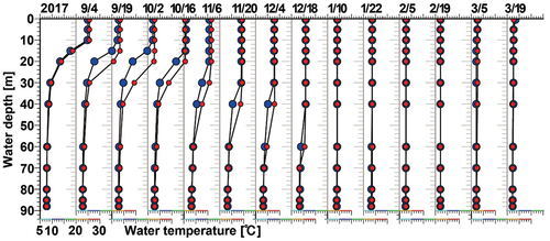
Figure A4. Vertical profiles of the simulated (larger blue dots) and observed water temperatures (red dots) in 2018/2019 at 17B (Fig. 1) during the cooling period from September to March.

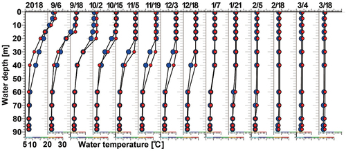
Figure A5. Vertical profiles of RMSE between the simulated and observed water temperature at 17B (Fig. 1) during the cooling period from September to March in 2017/2018 and 2018/2019.

References

- Adrian, R., et al., 2009. Lakes as sentinels of climate change. Limnology and Oceanography, 54 (6, part2), 2283–2297. doi:10.4319/lo.2009.54.6_part_2.2283
- Akitomo, K., Kurogi, M., and Kumagai, M., 2004. Numerical study of a thermally induced gyre system in Lake Biwa. Limnology, 5 (2), 103–114. doi:10.1007/s10201-004-0122-9
- Akitomo, K., Tanaka, K., and Kumagai, M., 2009a. Annual cycle of circulations in Lake Biwa, part 2: mechanisms. Limnology, 10 (2), 119–129. doi:10.1007/s10201-009-0268-6
- Akitomo, K., et al., 2009b. Annual cycle of circulations in Lake Biwa, part 1: model validation. Limnology, 10 (2), 105–118. doi:10.1007/s10201-009-0267-7
- Amadori, M., et al., 2021. Multi-scale evaluation of a 3D lake model forced by an atmospheric model against standard monitoring data. Environmental Modelling and Software, 139, 105017. doi:10.1016/j.envsoft.2021.105017
- Ambrosetti, W. and Barbanti, L., 1999. Deep water warming in lakes: an indicator of climate change. Journal of Limnology, 58 (1), 1–9. doi:10.4081/jlimnol.1999.1
- Arai, T., 1962. On the distribution of monthly mean bowen’s ratio for Inland and coastal sea waters in Japan. Journal of Agricultural Meteorology, 18 (2), 66–74. doi:10.2480/agrmet.18.66
- Arai, T., 2009. Climate change and variations in the water temperature and ice cover of inland waters. Japanese Journal of Limnology, 70, 99–116.
- Arhonditsis, G.B., et al., 2004. Effects of climatic variability on the thermal properties of Lake Washington. Limnology and Oceanography, 49 (1), 256–270. doi:10.4319/lo.2004.49.1.0256
- Binyamin, J., et al., 2006. Surface energy balance calculations for small northern lakes. International Journal of Climatology, 26 (15), 2261–2273. doi:10.1002/joc.1365
- Colomer, J., Roget, E., and Casamitjana, X., 1996. Daytime heat balance for estimating non‐radiative fluxes of Lake Banyoles, Spain. Hydrological Processes, 10 (5), 721–726. doi:10.1002/(SICI)1099-1085(199605)10:5<721::AID-HYP314>3.0.CO;2-0
- Desai, A.R., et al., 2009. Stronger winds over a large lake in response to weakening air-to-lake temperature gradient. Nature Geoscience, 2 (12), 855–858. doi:10.1038/ngeo693
- Duan, Z. and Bastiaanssen, W.G.M., 2015. A new empirical procedure for estimating intra-annual heat storage changes in lakes and reservoirs: review and analysis of 22 lakes. Remote Sensing of Environment, 156, 143–156. doi:10.1016/j.rse.2014.09.009
- Endoh, S. and Okumura, Y., 1993. Gyre system in Lake Biwa derived from recent current measurements. Japanese Journal of Limnology, 54 (3), 191–197.
- Ficker, H., Luger, M., and Gassner, H., 2017. From dimictic to monomictic: empirical evidence of thermal regime transitions in three deep alpine lakes in Austria induced by climate change. Freshwater Biology, 62 (8), 1335–1345. doi:10.1111/fwb.12946
- Foley, B., et al., 2012. Long-term changes in oxygen depletion in a small temperate lake: effects of climate change and eutrophication. Freshwater Biology, 57 (2), 278–289. doi:10.1111/j.1365-2427.2011.02662.x
- Garvine, R.W., 1999. Penetration of buoyant coastal discharge onto the continental shelf: a numerical model experiment. Journal of Physical Oceanography, 29 (8), 1892–1909. doi:10.1175/1520-0485(1999)029<1892:POBCDO>2.0.CO;2
- Gent, P.R. and Mcwilliams, J.C., 1990. Isopycnal mixing in ocean circulation models. Journal of Physical Oceanography, 20 (1), 150–155. doi:10.1175/1520-0485(1990)020<0150:IMIOCM>2.0.CO;2
- Gill, A.E., 1982. Atmosphere-ocean dynamics. San Diego: Academic Press.
- Haga, H., et al., 2007. Echosounding observations of coverage, height, PVI, and biomass of submerged macrophytes in the southern basin of Lake Biwa, Japan. Limnology, 8 (2), 95–102. doi:10.1007/s10201-006-0200-2
- Hirose, N., 2011. Inverse estimation of empirical parameters used in a regional ocean circulation model. Journal of Oceanography, 67 (3), 323–336. doi:10.1007/s10872-011-0041-4
- Hirose, N., et al., 2007. Sequential forecasting of the surface and subsurface conditions in the Japan Sea. Journal of Oceanography, 63 (3), 467–481. doi:10.1007/s10872-007-0042-5
- Hirose, N., et al., 2017. Numerical simulation of the abrupt occurrence of strong current in the southeastern Japan Sea. Continental Shelf Research, 143, 194–205. doi:10.1016/j.csr.2016.07.005
- Hirose, N., Kim, C.H., and Yoon, J.H., 1996. Heat budget in the Japan Sea. Journal of Oceanography, 52 (5), 553–574. doi:10.1007/BF02238321
- Ikebuchi, S., Seki, M., and Ohtoh, A., 1988. Evaporation from Lake Biwa. Journal of Hydrology, 102 (1–4), 427–449. doi:10.1016/0022-1694(88)90110-2
- Ishizaki, H. and Motoi, T., 1999. Reevaluation of the takano–oonishi scheme for momentum advection on bottom relief in ocean models. Journal of Atmospheric and Oceanic Technology, 16 (12), 1994–2010. doi:10.1175/1520-0426(1999)016<1994:ROTTOS>2.0.CO;2
- Ito, N., 1960. On the evaporation from a few Lakes in Japan. Journal of the Meteorological Society of Japan, 38 (4), 200–206. Ser. II. doi:10.2151/jmsj1923.38.4_200
- Ito, Y. and Momii, K., 2015. Impacts of regional warming on long‐term hypolimnetic anoxia and dissolved oxygen concentration in a deep lake. Hydrological Processes, 29 (9), 2232–2242. doi:10.1002/hyp.10362
- Jeon, C., Park, J.H., and Park, Y.G., 2019. Temporal and spatial variability of near‐inertial waves in the East/Japan sea from a high‐resolution wind‐forced ocean model. Journal of Geophysical Research: Oceans, 124 (8), 6015–6029. doi:10.1029/2018JC014802
- Kawamura, H., Yoon, J.H., and Ito, T., 2007. Formation rate of water masses in the Japan Sea. Journal of Oceanography, 63 (2), 243–253. doi:10.1007/s10872-007-0025-6
- Kawanabe, H., Nishino, M., and Maehata, M., eds., 2012. Lake Biwa: interactions between nature and people. Springer Science & Business Media.
- Keijman, J.Q., 1974. The estimation of the energy balance of a lake from simple weather data. Boundary-Layer Meteorology, 7 (3), 399–407. doi:10.1007/BF00240841
- Kim, C.H. and Yoon, J.H., 1999. A numerical modeling of the upper and the intermediate layer circulation in the East Sea. Journal of Oceanography, 55 (2), 327–345. doi:10.1023/A:1007837212219
- Kitazawa, D., 2011. Numerical simulation of long-term changes in water quality in deep lakes. Seisan Kenkyu, 63 (1), 65–68.
- Kitazawa, D., Kumagai, M., and Hasegawa, N., 2010. Effects of internal waves on dynamics of hypoxic waters in Lake Biwa. Journal of the Korean Society for Marine Environment & Energy, 13 (1), 30–42.
- Kitazawa, D., et al., 2018. Comparative study on vertical circulation in deep lakes: Lake Biwa and Lake Ikeda. In: 2018 OCEANS-MTS/IEEE Kobe Techno-Oceans (OTO), 1–4.
- Komatsu, T., Fukushima, T., and Harasawa, H., 2007. A modeling approach to forecast the effect of long-term climate change on lake water quality. Ecological Modelling, 209 (2–4), 351–366. doi:10.1016/j.ecolmodel.2007.07.021
- Kondo, J., 1975. Air-sea bulk transfer coefficients in diabatic conditions. Boundary-Layer Meteorology, 9 (1), 91–112. doi:10.1007/BF00232256
- Kondo, J. and Watanabe, T., 1992. Studies on the bulk transfer coefficients over a vegetated surface with a multilayer energy budget model. Journal of the Atmospheric Sciences, 49 (23), 2183–2199. doi:10.1175/1520-0469(1992)049<2183:SOTBTC>2.0.CO;2
- Koreeda, N., et al., 2003. Applicability of JMA-MSM-GPV to river basin risk management and disaster measures. Proceedings of Hydraulic Engineering, 47, 91–96. doi:10.2208/prohe.47.91
- Koue, J., et al., 2018a. Evaluation of thermal stratification and flow field reproduced by a three-dimensional hydrodynamic model in Lake Biwa, Japan. Water, 10 (1), 47. doi:10.3390/w10010047
- Koue, J., et al., 2018b. Numerical analysis of sensitivity of structure of the stratification in Lake Biwa, Japan by changing meteorological elements. Water, 10 (10), 1492. doi:10.3390/w10101492
- Koue, J., et al., 2018c. Numerical assessment of the impact of strong wind on thermal stratification in Lake Biwa, Japan. International Journal of Geomate, 14 (45), 35–40. doi:10.21660/2018.45.7166
- Kumagai, M., Maeda, H., and Oonishi, Y., 1986. Vertical circulation and formation of anoxic layer - case study at dredged area in southern basin of Lake Biwa (in Japanese). Japanese Journal of Limnology, 47 (1), 27–35.
- Lee, H.J., et al., 2003. Comparison of riamom and mom in modeling the East Sea/Japan Sea circulation. Ocean and Polar Research, 25 (3), 287–302. doi:10.4217/OPR.2003.25.3.287
- Lewis, J. and William, M., 1983. A revised classification of lakes based on mixing. Canadian Journal of Fisheries and Aquatic Sciences, 40 (10), 1779–1787. doi:10.1139/f83-207
- Li, M., Zhong, L., and Boicourt, W.C., 2005. Simulations of Chesapeake Bay estuary: sensitivity to turbulence mixing parameterizations and comparison with observations. Journal of Geophysical Research: Oceans, 110 (C12), C12004.
- Livingstone, D.M., 2003. Impact of secular climate change on the thermal structure of a large temperate central European lake. Climatic Change, 57 (1/2), 205–225. doi:10.1023/A:1022119503144
- Magee, M.R. and Wu, C.H., 2017. Response of water temperatures and stratification to changing climate in three lakes with different morphometry. Hydrology and Earth System Sciences, 21 (12), 6253. doi:10.5194/hess-21-6253-2017
- Martínez-Alvarez, V., et al., 2011. Simultaneous solution for water, heat and salt balances in a Mediterranean coastal lagoon (Mar Menor, Spain). Estuarine, Coastal and Shelf Science, 91 (2), 250–261. doi:10.1016/j.ecss.2010.10.030
- Matsumoto, K., Tokos, K.S., and Rippke, J., 2019. Climate projection of Lake Superior under a future warming scenario. Journal of Limnology, 78 (3), 296–309. doi:10.4081/jlimnol.2019.1902
- Mellor, G.L., 1998. Users guide for a three dimensional, primitive equation, numerical ocean model. Program in Atmospheric and Oceanic Sciences. Princeton, NJ: Princeton University. http://www.aos.princeton.edu/WWWPUBLIC/htdocs.pom/ [Accessed 29 Jun 2023].
- Momii, K. and Ito, Y., 2008. Heat budget estimates for lake Ikeda, Japan. Journal of Hydrology, 361 (3–4), 362–370. doi:10.1016/j.jhydrol.2008.08.004
- Moon, J.H., et al., 2009. Effect of the along-strait wind on the volume transport through the Tsushima/Korea Strait in september. Journal of Oceanography, 65 (1), 17–29. doi:10.1007/s10872-009-0002-3
- Moriasi, D.N., et al., 2007. Model evaluation guidelines for systematic quantification of accuracy in watershed simulations. Transactions of the ASABE, 50 (3), 885–900. doi:10.13031/2013.23153
- Murphy, A.H. and Epstein, E.S., 1989. Skill scores and correlation coefficients in model verification. Monthly Weather Review, 117 (3), 572–582. doi:10.1175/1520-0493(1989)117<0572:SSACCI>2.0.CO;2
- Nakada, S., et al., 2021. High-resolution flow simulation in Typhoon 21, 2018: massive loss of submerged macrophytes in Lake Biwa. Progress in Earth and Planetary Science, 8 (1), 1–19. doi:10.1186/s40645-021-00440-9
- Nakada, S., et al., 2014. Operational ocean prediction experiments for smart coastal fishing. Progress in Oceanography, 121, 125–140. doi:10.1016/j.pocean.2013.10.008
- Nakada, S., et al., 2013. An integrated approach to the heat and water mass dynamics of a large bay: high‐resolution simulations of Funka Bay, Japan. Journal of Geophysical Research: Oceans, 118 (7), 3530–3547. doi:10.1002/jgrc.20262
- Nakada, S., et al., 2012. Modeling runoff into a region of freshwater influence for improved ocean prediction: application to Funka Bay. Hydrological Research Letters, 6, 47–52. doi:10.3178/hrl.6.47
- Nakada, S., et al., 2010. A study of the dynamic factors of the summer-time upwelling in the Tsushima warm current region. Deep Sea Research Part II: Topical Studies in Oceanography, 57 (19–20), 1799–1808. doi:10.1016/j.dsr2.2010.04.006
- Noh, Y., Min, H.S., and Raasch, S., 2004. Large eddy simulation of the ocean mixed layer: the effects of wave breaking and Langmuir circulation. Journal of Physical Oceanography, 34 (4), 720–735. doi:10.1175/1520-0485(2004)034<0720:LESOTO>2.0.CO;2
- North, R.P., et al., 2014. Long-term changes in hypoxia and soluble reactive phosphorus in the hypolimnion of a large temperate lake: consequences of a climate regime shift. Global Change Biology, 20 (3), 811–823. doi:10.1111/gcb.12371
- O’Reilly, C.M., et al., 2003. Climate change decreases aquatic ecosystem productivity of Lake Tanganyika, Africa. Nature, 424 (6950), 766–768. doi:10.1038/nature01833
- Obata, A., Ishizaka, J., and Endoh, M., 1996. Global verification of critical depth theory for phytoplankton bloom with climatological in situ temperature and satellite ocean color data. Journal of Geophysical Research: Oceans, 101 (C9), 20657–20667. doi:10.1029/96JC01734
- Piccolroaz, S., et al., 2019. Importance of planetary rotation for ventilation processes in deep elongated lakes: evidence from Lake Garda (Italy). Scientific Reports, 9 (1), 8290. doi:10.1038/s41598-019-44730-1
- Piccolroaz, S. and Toffolon, M., 2018. The fate of Lake Baikal: how climate change may alter deep ventilation in the largest lake on Earth. Climatic Change, 150 (3–4), 181–194. doi:10.1007/s10584-018-2275-2
- Reed, R.K., 1977. On estimating insolation over the ocean. Journal of Physical Oceanography, 7 (3), 482–485.e. doi:10.1175/1520-0485(1977)007<0482:OEIOTO>2.0.CO;2
- Rouse, W.R., et al., 2003. Interannual and seasonal variability of the surface energy balance and temperature of central Great Slave Lake. Journal of Hydrometeorology, 4 (4), 720–730. doi:10.1175/1525-7541(2003)004<0720:IASVOT>2.0.CO;2
- Sahoo, G.B., Schladow, S.G., and Reuter, J.E., 2013. Hydrologic budget and dynamics of a large oligotrophic lake related to hydro-meteorological inputs. Journal of Hydrology, 500, 127–143. doi:10.1016/j.jhydrol.2013.07.024
- Sasajima, Y.I., et al., 2007. Structure of the subsurface counter current beneath the Tsushima warm current simulated by an ocean general circulation model. Journal of Oceanography, 63 (6), 913–926. doi:10.1007/s10872-007-0077-7
- Sato, Y., et al., 2011. Construction and validation of Lake Biwa basin simulation model with integration of three components of land, Lake flow, and Lake ecosystem. Journal of Japan Society on Water Environment, 34 (9), 125–141. doi:10.2965/jswe.34.125
- Shatwell, T., Thiery, W., and Kirillin, G., 2019. Future projections of temperature and mixing regime of European temperate lakes. Hydrology and Earth System Sciences, 23 (3), 1533–1551. doi:10.5194/hess-23-1533-2019
- Smedstad, O.M., et al., 2003. An operational eddy resolving 1/16 global ocean nowcast/forecast system. Journal of Marine Systems, 40, 341–361. doi:10.1016/S0924-7963(03)00024-1
- Stetler, J.T., et al., 2021. Atmospheric stilling and warming air temperatures drive long-term changes in lake stratification in a large oligotrophic lake. Limnology and Oceanography, 66 (3), 954–964. doi:10.1002/lno.11654
- Suda, K., 1926. The report of limnological observation in Lake Biwa-ko (I). Bull Kobe Marine Obs, 8, 1–103.
- Swann, G.E.A., et al., 2020. Changing nutrient cycling in Lake Baikal, the world’s oldest lake. Proceedings of the National Academy of Sciences, 117 (44), 27211–27217. doi:10.1073/pnas.2013181117
- Talling, J.F., 2001. Environmental controls on the functioning of shallow tropical lakes. Hydrobiologia, 458 (1–3), 1–8. doi:10.1023/A:1013121522321
- Taniguchi, M., et al., 2000. Stable isotope studies of precipitation and river water in the Lake Biwa basin, Japan. Hydrological Processes, 14 (3), 539–556. doi:10.1002/(SICI)1099-1085(20000228)14:3<539::AID-HYP953>3.0.CO;2-L
- Valerio, G., et al., 2015. Sensitivity of the multiannual thermal dynamics of a deep pre‐alpine lake to climatic change. Hydrological Processes, 29 (5), 767–779. doi:10.1002/hyp.10183
- Wang, M., et al., 2021. Changes in the lake thermal and mixing dynamics on the Tibetan Plateau. Hydrological Sciences Journal, 66 (5), 838–850. doi:10.1080/02626667.2021.1887487
- Woolway, R.I., et al., 2017. Atmospheric stilling leads to prolonged thermal stratification in a large shallow polymictic lake. Climatic Change, 141 (4), 759–773. doi:10.1007/s10584-017-1909-0
- Woolway, R.I. and Merchant, C.J., 2019. Worldwide alteration of lake mixing regimes in response to climate change. Nature Geoscience, 12 (4), 271–276. doi:10.1038/s41561-019-0322-x
- Xing, Z., et al., 2012. Water and heat budgets of a shallow tropical reservoir. Water Resources Research, 48 (6), 6. doi:10.1029/2011WR011314
- Yamada, K., et al., 2021. First observation of incomplete vertical circulation in Lake Biwa. Limnology, 22 (2), 179–185. doi:10.1007/s10201-021-00653-3
- Yankova, Y., et al., 2017. Abrupt stop of deep water turnover with lake warming: drastic consequences for algal primary producers. Scientific Reports, 7 (1), 1–9. doi:10.1038/s41598-017-13159-9
- Yoshida, T., et al., 2018. Numerical simulation of overturn in Lake Biwa and its relation to climate change. Seisan Kenkyu, 70 (1), 25–28.
- Yoshimizu, C., et al., 2010. Vulnerability of a large monomictic lake (Lake Biwa) to warm winter event. Limnology, 11 (3), 233–239. doi:10.1007/s10201-009-0307-3