Assessing robustness in global hydrological predictions by comparing modelling and Earth observations

ABSTRACT

Hydrological modelling to support hypotheses on Earth system boundaries or the accelerating water crisis is nowadays done at the global scale, with difficulties associated to model uncertainties. Here we bring a robustness analysis of internal model variables as an additional tool for model evaluation using data from six Earth observation products and the global catchment model World-Wide HYPE in a comparative study. The assessment shows that: (i) variables have high agreement in mid-latitude temperate regions; (ii) the variables with higher agreement, and associated with good model performance in streamflow, were actual evapotranspiration, fractional snow cover and snow water equivalent; and (iii) changes in total water storage showed very poor agreement, probably due to an insufficient number of aquifers in the model set-up. We propose this procedure as a standard complementary method in global hydrological modelling, highlighting the importance of justifying models before using them for scenario analysis or water accounting.

KEYWORDS:

• global hydrological modelling evaluation
• water cycle
• model-based robustness analysis
• multi-variable estimation
• Earth observations
• UPH 16

Editor A. Fiori; Associate Editor K. Soulis

1 Introduction

The first global hydrological model (GHM) appeared in 1989 and described the global hydrological cycle in broad terms (Sood and Smakhtin 2015). Since then, different modelling communities followed, using different discretization schemes and approaches to describe dynamics of hydrological variables (Bierkens et al. 2015) and develop GHMs or continental models for different purposes (Archfield et al. 2015). For instance, hydrological communities moved towards global water security modelling (Arnell 1999, Vörösmarty et al. 2000, Döll et al. 2003) as well as forecasting river flow at the global scale (e.g. Alfieri et al. 2023, Harrigan et al. 2023).

Meanwhile, the climate community moved towards Earth system models with improved hydrological components (e.g. Tang et al. 2007, Rost et al. 2008, Pokhrel et al. 2014, Wada et al. 2014), and the meteorological land-surface community coupled atmospheric and water cycle processes (e.g. Liang et al. 1994, Best et al. 2011, Guimberteau et al. 2012) for integrated forecasting. All these global models are gridded and many are not calibrated or evaluated against streamflow observations but rather are used in multi-model ensembles. Accordingly, recent systematic evaluation of several such GHMs found weak to poor performance of river discharge in many basins around the globe (Gädeke et al. 2020, Krysanova et al. 2020).

The catchment hydrology community, with a long tradition in calibrating and evaluating hydrological models, has traditionally worked at scales up to the river basin. Thanks to the increasing computational capacity as well as the growing trend towards open data, catchment modelling has now expanded to also encompass continental scales (Widén-Nilsson et al. 2007, Pechlivanidis and Arheimer 2015, Donnelly et al. 2016). Along these lines, Arheimer et al. (2020) set up the Hydrological Prediction for the Environment (HYPE) model, a process-oriented semi-distributed hydrological model, at the global scale. World-Wide HYPE (WWH) uses openly accessible data, such as river discharge after quality checks (Crochemore et al. 2020), and all datasets required for the catchment delineation, soil, and land use classification, and model forcing. The stepwise calibration strategy used in the set-up of WWH was designed to represent river discharge worldwide (Arheimer et al. 2020).

Nevertheless, the goal of GHMs is broader than just simulating streamflow; they also aim at supporting hypotheses about Earth system boundaries (Rockström et al. 2023) or how to manage the accelerating water crisis (e.g. Hoekstra et al. 2012, Bierkens et al. 2021, GCEW 2023). This demands an understanding of the global water cycle and reproducing the different water cycle components in addition to river discharge, for instance global evapotranspiration (Pimentel et al. 2023), runoff from soils (Santos et al. 2022) or groundwater fluxes (De Graaf et al. 2019). It is well known that correctly reproducing river discharge does not guarantee that other hydrological state variables and fluxes in a catchment are correctly represented; models may reproduce river discharge well, but not for the correct reasons (Kirchner 2006), which could be due to the problem of equifinality (Beven 2006, Muñoz et al. 2014, Her and Chaubey 2015). Therefore, evaluating internal variables in hydrological models is important to ensure the correct representation of the different water cycle components (Montanari et al. 2008, Lindström et al. 2010, Rakovec et al. 2016, Li et al. 2018).

Nowadays, another independent source of data is available from Earth observation (EO). The huge efforts made in the last few decades to observe the Earth from space have made accessible a sizeable number of products representing hydrological variables (mostly covering at least the last decade). For instance, potential and actual evapotranspiration (PET and AET; Mu et al. 2011), snow cover (Hall et al. 2002), snow water equivalent (SWE; Takala et al. 2011), soil moisture (SM; Dorigo et al. 2017) or changes in water storage (ΔS; Han et al. 2005) are some of the hydrological variables retrieved from EO. Sometimes, the spatiotemporal resolution of these products makes their use at the local scale difficult; however, they offer great opportunities at the global scale.

Even though this remote sensing information is usually referred to as observation, in most cases the final variable provided is based on post-processing and combination with other datasets. For instance, EO-based evapotranspiration is derived from surface temperature observations, using meteorological information and specific assumptions about vegetation cover (Mu et al. 2007); soil moisture is derived from microwave information assuming changes in the dielectric constant (Notarnicola et al. 2008); and ΔS values are derived from variation in the gravity field (Landerer and Swenson 2012). Therefore, these products include not only uncertainties due to the measuring devices, but also uncertainties related to the algorithms used for translating the observed magnitudes to the final hydrological variables. Here, we will refer to these data as “EO products” to underline that they are not direct observations, and uncertainties are intrinsically included in all of them, just like in hydrological models.

There is a clear need to assess the performance of GHMs using streamflow data (e.g. Krysanova et al. 2018, 2020). In addition, we propose that an in-depth assessment of GHMs against not only streamflow but also remote-sensing information would help ensure that model results are robust. Since both hydrological models and the EO products have uncertainties and constitute a combination of direct measurements and equations, we do not aim to evaluate them against each other. Doing so would assume that one is inherently more trustworthy than the other, which is sometimes done in hydrological studies (e.g. Xu et al. 2014, Rajib et al. 2016, Demirel et al. 2018, Huang et al. 2018, Han et al. 2019, Dile et al. 2020). We prefer to consider both datasets as plausible quantifications of a certain variable.

Therefore, we propose to assess the degree to which these quantifications agree or correspond as an indicator of the results’ robustness (see definitions by e.g. Lloyd 2015, Schupbach 2018, Harris and Frigg 2023). Thus, we define a variable as robust if there is agreement on it among several independent data sources (e.g. river gauges, process-based modelling, EO products) at the global scale. Such robustness would give more confidence when using hydrological model results, for instance in impact analysis (e.g. climate scenarios), operational hydrological forecasts, and understanding global hydrological storages and fluxes. Finding robust variables calls for a multi-source and multi-variable analysis. In this context, the main objectives of this study are twofold: first, to compare estimates of hydrological variables from WWH and EO products to assess the robustness of results; and, second, to promote the concept of evaluating GHMs in the light of EO products and thereby go beyond in situ river discharge observations to multi-variable estimation of the water cycle.

This work examines research question No. 16 of the 23 unsolved problems in hydrology (UPH; Blöschl et al. 2019): “How can we use innovative technologies to measure surface and subsurface properties, states, and fluxes, at a range of spatial and temporal scales?” p. 1148.

2 Data

We compared estimates of six hydrological variables from two types of data sources for the period 2000–2014 (Table 1): EO and dynamically modelled outputs from the GHM WWH. The procedures on how to estimate the hydrological variables in the model and in each EO product are presented below.

Table 1. Earth observation (EO) products, and World-wide HYPE (WWH) results.

	Product/model variable		Spatial resolutions		Temporal resolution
Variable	EO product	WWH v. 1.3	EO product	WWH (km^2)	EO product	WWH
Potential evapotranspiration (PET)	MOD16	epot	1 × 1 km	~1000*	Monthly	Daily
Actual evapotranspiration (AET)	MOD16	evap	1 × 1 km	~1000*	Monthly	Daily
Fractional snow cover (FSC)	MOD10CM	cfsc	0.05 × 0.05°	~1000*	Monthly	Daily
Snow water equivalent (SWE)	SWE-GLOBSNOW	snow	25 × 25 km	~1000*	Monthly	Daily
Soil moisture in the top layer (~25 cm) (SM)	ESA-CCI SM	sml1	25 × 25 km	~1000*	Daily	Daily
Changes in water storage ($\mathrm{\Delta }$ S)	GRACE Tellius	ΔS	1 × 1°	~1000*	Monthly	Daily

*Mean size of 1020 km² (5th percentile: 64 km²; 50th percentile: 770 km²; 95th percentile: 2185 km²).

2.1 Potential evapotranspiration

PET is a concept commonly used in hydrology as an intermediate component describing the energy-based demand when calculating AET. PET is defined as the evaporation from a vegetated surface with an unlimited amount of water available and without advection or heat-storage effects (Thornthwaite 1948). We use the moderate resolution imaging spectroradiometer (MODIS) global PET product (MOD16; Mu et al. 2007, 2011) at monthly resolution for EO, which is the most standardized remote-sensing-based evapotranspiration product at global scale. MOD16 is based on the Penman-Monteith equation (Penman 1948, Monteith 1965), which combines energy and water balance using standard climatological records, such as radiation, temperature, humidity, and wind speed, and introducing aerodynamics and surface resistance from the vegetation canopy. Due to its physical parameterization, this product needs a high number of input datasets to calculate the final evapotranspiration. These include remote sensing products and meteorological data.

The remote sensing products it utilizes are: (1) collection 5 climate modellling grid (CMG) MODIS albedo band 10 from MOD43C1 (Schaaf et al. 2002, Jin et al. 2003, Salomon et al. 2006); (2) global collection 4 MODIS land cover type 2 (MOD12Q1; Friedl et al. 2002) and (3) global MODIS collection 5 of fraction of photosynthetically active radiation (FPAR) and leaf area index (LAI) (MOD15A2; Myneni et al. 2002). Daily air pressure, air temperature, humidity, and radiation from the reanalysis product of the Global Modelling and Assimilation Office (GMAO) are used as meteorological forcing (see Mu et al. 2011 for specific details). The final PET provided by the MOD16 product is calculated as the sum of the evaporation from rain intercepted by the canopy before it reaches the soil, the potential plant transpiration, the evaporation from wet soil and the PET from the soil components. The MODIS PET product has been assessed by comparison with other distributed PET estimates (Velpuri et al. 2013, Faisol et al. 2020). However, its accuracy is highly dependent on the meteorological data and the PET equation used in the calculation.

In WWH, PET (epot in HYPE terminology) is calculated using three different model equations: (1) the Jensen-Haise equation (Jensen and Haise 1963) in temperate areas; (2) the modified Hargreaves equation (Hargreaves and Samani 1982) in tropical and arid areas; and (3) the Priestley-Taylor equation (Priestley and Taylor 1972) in snow/ice-dominated regions. These algorithms have been judged the most appropriate in previous HYPE set-ups in the selected regions (Donnelly et al. 2016, Andersson et al. 2017, MacDonald et al. 2018). Equation parameters for PET calculations have been estimated for each hydrological response unit, (HRU; corresponding to different land cover) using river discharge from representative gauged catchments (Arheimer et al. 2020, Santos et al. 2022).

2.2 Actual evapotranspiration

MOD16 was also used as the remote sensing-based product for AET. The Penman-Monteith equation is behind this product (see Section 2.1). However, in this case, the final AET is calculated as the sum of different evaporation components: evaporation losses from the wet canopy, actual plant transpiration and actual soil evaporation. This product was validated against eddy covariance measurements worldwide, with varying results in terms of accuracy (Hu et al. 2015). For instance, Mu et al. (2011) showed a mean bias in daily AET of 0.31 mm/day⁻¹ at 46 sites in North America. In South America, Ruhoff et al. (2013) found that the relative error (RE) in AET was about 19% at two sites over the Rio Grande (Brazil). In Europe, Hu et al. (2015) obtained correlation coefficients ranging within the interval 0.45–0.98 and a mean bias within the interval −0.9 to 1.11 mm/day⁻¹. In Asia, Kim et al. (2012) found AET correlations ranging from 0.27 to 0.82 and biases ranging from −24 to 2.3 mm/8 days⁻¹, over 17 sites.

In WWH, AET (evap in HYPE terminology) may occur from the two topsoil layers (some 1–2 m depending on the HRU), considered as the plant rooting depth. In each layer, AET is assumed equal to PET if the soil moisture is above a certain threshold (field capacity) and decreases until the zero-evaporation threshold is reached (wilting point). The AET is assumed to decrease exponentially with depth and is divided between the two layers. AET is set to zero for temperatures below a certain threshold and for negative PET estimation (Lindström et al. 2010). For the HRU corresponding to water bodies (e.g. rivers, floodplains, and lakes), AET is assumed equal to PET when the air temperature is above a certain threshold. This evaporation is limited by the volume of water in the water body.

2.3 Fractional snow cover

For fractional snow cover (FSC) we used MOD10CM, which is a global 0.05 × 0.05° resolution monthly mean snow cover extent product derived from the daily equivalent MOD10C1 (Hall and Riggs 2007). Two filters are applied to consider only relevant days in the monthly mean estimation. The first filter is used to remove days with high cloud coverage. A daily clear index (CI) is defined and only days above a threshold (70%) are used in the monthly mean. The second filter is applied to filter out the cells in which the snow cover extent is less than a threshold (10%). Similarly, the daily FSC product, MOD10C1, has spatial aggregation at 0.05 × 0.05° of the 500 × 500 m daily MOD10A1, which contains the original snow cover extension in terms of normalized difference snow index (NDSI; Dozier 1989). This index is calculated based on the physical properties of snow.

Snow has a very high reflectance in the visible region and very low reflectance in the shortwave infrared region of the electromagnetic spectrum. A cell with an NDSI value greater than zero is considered to have some snow presence. The NDSI from MOD10A1 is interpreted as a binary map to build the MOD10C1 product. MODIS snow products have been substantially assessed against ground data. An overall accuracy of about 93%, with variations by land-cover type and snow condition, was reported by Hall and Riggs (2007). In mountain areas these accuracies depend less on land-cover type and more on the period of the year (Parajka et al. 2012, Notarnicola et al. 2013). The errors are usually lower in winter than in spring (Gascoin et al. 2015, Pimentel et al. 2018). In addition, Hall and Riggs (2017) stated that MOD10CM, compared to other monthly snow maps, tends to better agree during the winter months than in the fall when snow is accumulating.

WWH calculates FSC (cfsc in HYPE terminology) based on the methodology of Samuelsson et al. (2011). The snow cycle is divided in three phases: (1) an accumulation phase in which the snow cover increases as function of the SWE to a maximum extent threshold; (2) a consolidation phase, in which the snow cover extent is redistributed based on topographic characteristics of the HRU (e.g. mean elevation and standard deviation of this elevation) and the maximum extent is reached; (3) a melting phase, in which the snow cover extent decreases exponentially. For seasons when the snowpack does not reach the definition of large snowpack, the first equation is used during the whole season.

2.4 Snow water equivalent

The Global Snow Monitoring for Climate Research (GlobSnow v. 2.0; Takala et al. 2011) is used as the remote sensing source for SWE. This product is based on a retrieval algorithm that assimilates synoptic weather station data on snow depth with satellite passive microwave radiometer data from the Scanning Multi-channel Microwave Radiometer (SMMR), Special Sensor Microwave Imager (SSM/I) and Special Sensor Microwave Imager/Sounder (SSMIS) sensors (Pulliainen et al. 1999, Takala et al. 2011). Daily, weekly, and monthly time series of SWE, covering more than 30 years, are produced at 25 km resolution over the Northern Hemisphere (latitudes ranging from 35° to 85°), except for mountainous areas and Greenland, due to limitations in the satellite information and retrieval algorithm. The monthly product was used in this study. The retrieval accuracy of GlobSnow SWE product was evaluated against 1264 different snow survey locations in Russia (Hancock et al. 2013). The comparison showed a root mean square error of 32.5 mm for snowpacks with SWE values ranging between 0 and 150 mm; this error increases to 43.5 mm when including all snowpacks analysed (Luojus et al. 2016). GlobSnow SWE product was also evaluated using snow surveys in Finland and Canada, with root mean square errors of 30 and 100 mm, respectively (Mortimer et al. 2020).

In WWH, all precipitation falling under a temperature threshold is considered to be snow and is added to the snowpack. Moreover, a portion of the precipitation happening within a temperature range centred on this temperature threshold is also defined as snow and added to the snowpack. SWE losses occur by evaporation and melting. Evaporation from the snowpack is calculated as a fraction of the PET in each catchment, which is calibrated for each HRU in the model. Snowmelt is a function of two melting ratios, that are temperature- and radiation-dependent, respectively. A snow cover scaling is also applied in each catchment to only consider covered areas.

2.5 Soil moisture

SM from the European Space Agency (ESA) CCI SM (ESA multi-decadal, global satellite-derived dataset as part of the Climate Change Initiative programme; Dorigo et al. 2017) is used as the remote sensing source data. Here we used the COMBINED product, which is a combination of active and passive microwave products and was found to outperform the single sensor input products (Dorigo et al. 2017). The ESA CCI SM COMBINED product has global coverage, daily temporal resolution and 25 × 25 km grid size. There is no clear agreement on the soil depth that these products can represent; however, several studies suggested that the SM measurements could be extrapolated to 20–25 cm (Zeng et al. 2015, Wigneron et al. 2017, Ma et al. 2019). The product provides several uncertainty flags for removing possible errors in measurements and retrieval, which we have considered as a quality check of the data. The overall accuracy, which was calculated as unbiased root mean square error, of the ESA CCI SM product is 0.04 m³m⁻³. Moreover, based on various studies, Dorigo et al. (2017) concluded that this product generally matches in situ observation relatively well in temperate climates, over grassland and agricultural areas, and in semi-arid regions, but has difficulty reflecting the temporal dynamics in the driest and wettest areas.

In WWH, the SM is the result of the water balance in the soil. A fraction of the rainfall and snowmelt infiltrate into the topsoil, the remaining fraction being diverted into surface and macropore flows. This diversion only occurs if a maximum water content is exceeded. This maximum threshold in a soil layer is determined by three model parameters defined per layer that represent the total porosity of each layer. Soil moisture above the threshold may percolate down to the next layer. The percolation is determined by the soil type influencing the maximum percolation capacity and the available space in the soil layers below (Lindström et al. 2010, Arheimer et al. 2020). In WWH, the soil is divided into three layers (e.g. Santos et al. 2022). Here, we only used the water available in the first layer (sml1), which has a constant depth of 25 cm.

2.6 Variation in ΔS

Gravity Recovery and Climate Experiment (GRACE) Tellus Release 05 is the dataset used as the EO product to assess variations in water storage (ΔS). GRACE Tellus derives ΔS relative to a time-mean baseline measuring changes in the gravity field (Wahr et al. 1998), which can be mainly associated with variations in all hydrological storage. Here, we used, as recommended, the ensemble of the spherical harmonic data produced by three centres: the Center for Space Research (CSR), GeoForschungsZentrum (GFZ), and the Jet Propulsion Laboratory (JPL). This ensemble is multiplied by a scaling grid, which restores most of the energy removed by the Gaussian and degree 60 filters applied in the production of the spherical harmonic solutions and reduces uncertainties. These uncertainties, in terms of mean square error, are generally lower than 2 cm for large river basins and about 3–4 cm for smaller river basins (Landerer and Swenson 2012). GRACE Tellus has a global coverage of monthly data at 1° × 1° spatial resolution.

In WWH we derive the ΔS through a post-processing procedure applied to model outputs. All ΔS in the model (i.e. in aquifers, glaciers, lakes, floodplains, rivers, snow, and soil) are summarized for each catchment and aggregated to the monthly time scale. Monthly ΔS values are derived in relation to a reference baseline, which is calculated as the mean ΔS for the same years as the baseline in GRACE Tellus.

3 Methods

For each of the six hydrological variables listed in Table 1, EO and WWH time series were compared at the coarser scale. The PET, AET, FSC, SWE and SM from EO products were aggregated to the model’s spatial scale (on average ~1000 km²) by calculating spatial average values for each catchment and month, taking into consideration specific EO products’ warning flags. Hydrological model anomalies in ΔS were computed at GRACE resolution (1° × 1°).

The variables and analysis methods were chosen to examine the robustness in results from WWH for three main applications: (i) assessing long-term water resource availability under present and future climates, (ii) operational forecasting of seasonal variation in river discharge, and (iii) better understanding hydrological processes worldwide. First, connected to climate application, long-term means (defined as the means of the annual values during 2000–2014) were used in the analysis of raw EO and model values in terms of their relative difference formulated based on the RE:

(1) $RE=100\cdot \frac{x_{WWH}-x_{EO}}{x_{EO}}$(1)

where $x$ represents the long-term mean of the selected variable during the period 2000–2014, and the sub-indices EO and WWH represent the EO product and the WWH modelled hydrological variable, respectively. Positive (negative) values indicate that the WWH-modelled value is greater (smaller) than the EO product value.

Second, monthly means were used to assess the seasonal dynamics for each variable within the study period. This assessment was carried out using the statistical Kling-Gupta efficiency metric (KGE; Gupta et al. 2009; Equation (1))(1) $RE=100\cdot \frac{x_{WWH}-x_{EO}}{x_{EO}}$(1) and its components r, β and α (Equations (2)(2) $KGE=\sqrt{{\left(r-1\right)}^2+{\left(\alpha -1\right)}^2+{\left(\beta -1\right)}^2}$(2) –(4(4) $\beta =\frac{x_{WWH}}{x_{EO}};RE=\left(\beta -1\right)\cdot 100$(4) )). These components are related to the most common metrics used to assess model performance in catchment hydrology: Pearson correlation coefficient (CC), RE and relative error of standard deviation (RESD):

(2) $KGE=\sqrt{{\left(r-1\right)}^2+{\left(\alpha -1\right)}^2+{\left(\beta -1\right)}^2}$(2)

where:

(3) $r=CC=\frac{cov\left(x_{WWH},x_{EO}\right)}{{\sigma }_{WWH}{\sigma }_{EO}}$(3)

(4) $\beta =\frac{x_{WWH}}{x_{EO}};RE=\left(\beta -1\right)\cdot 100$(4)

(5) $\alpha =\frac{{\sigma }_{WWH}}{{\sigma }_{EO}};RESD=\left(\alpha -1\right)\cdot 100$(5)

and x represents the monthly time series of each variable, $x$ their long-term means, and $\sigma$ their standard deviations. The sub-indices EO and WWH represent the EO product and the WWH modelled hydrological variable, respectively.

Finally, connected to process understanding, we evaluated the relation between (i) the WWH model performance in terms of discharge and (ii) the agreement between EO products and internal WWH model variables. The WWH model had already been calibrated and evaluated using KGE as a metric for model performance between simulated and in situ river flow measurements at 5338 sites for the period 1981–2012 (Arheimer et al. 2020), of which 4367 sites where applicable in the current study for the time period with EO data (2000–2014). The results of Arheimer et al. (2020) show a median monthly KGE of 0.4 with spatial variations in model performance. For instance, better performances (KGE > 0.6) were found in Europe, Japan, Southeast Asia, and the USA, as well as in parts of Canada, Russia, and South America.

Moreover, the WWH model shows potential in reproducing several flow signatures (Arheimer et al. 2020), such as high monthly flows, spatial variability of high flows, duration of low flows, and constancy (see definition by Colwell 1974) of daily flow. Nevertheless, robust signals of additional hydrological model variables would indicate that the model represents river discharge for the right reasons. To analyse this, we grouped catchments globally into four groups based on their KGE value for discharge in the 4367 gauging stations with data available in the period 2000–2014, each group representing one quartile of the KGE distribution. In each group, the six internal variables (PET, ET, FSC, SWE, SM and $\mathrm{\Delta }S$) were assessed using the same metrics as described in Equations (1)(1) $RE=100\cdot \frac{x_{WWH}-x_{EO}}{x_{EO}}$(1) –(5(5) $\alpha =\frac{{\sigma }_{WWH}}{{\sigma }_{EO}};RESD=\left(\alpha -1\right)\cdot 100$(5) ).

4 Results and discussion

The results from comparing hydrological variables from GHM and EO products around the globe show both similarities and differences, which, in coherence with previous studies, are sometimes difficult to explain (cf. Döll et al. 2014, Bierkens et al. 2021). Nevertheless, we conducted a thorough analysis of the six variables studied with the ambition to learn about process representation. Below we discuss potential reasons for disagreements, and we found that uncertainties could be referred to both data sources.

In the discussion that follows, we use the term “robustness,” which has various meanings in science (O’Loughlin 2021). We examine our results from a model-based robustness analysis perspective, which is commonly used in climate science (Lloyd 2015, Schupbach 2018). According to this definition, a result is regarded as well supported if a sufficiently diverse set of models agree on it (Harris and Frigg 2023) when there is no “ground truth” available. Using this definition, we found the long-term mean of the variables PET, AET, FSC and SWE to be robust, SM to be semi-robust and ΔS to be weak. For seasonal dynamics, none of the variables were robust at the global scale (only regionally) except for PET. To a large extent this can be referred to uncertainties in the EO products, but also to the GHM (see below).

4.1 Long-term patterns

Comparison of annual means for the six variables from WWH and EO products, respectively, showed similarities in the global patterns but also major differences, which were quantified in relative terms (Fig. 1) and analysed as follows.

Figure 1. Comparison of the long-term annual means for the analysed period (2000–2014) of the six analysed variables (rows): potential evapotranspiration (PET), actual evapotranspiration (AET), fractional snow cover (FSC), snow water equivalent (SWE), soil moisture (SM), and changes in water storage (ΔS) for values simulated by World-wide HYPE (WWH; column 1), values from the selected Earth observation (EO) products (column 2) and relative difference (column 3). The relative difference uses the EO product as the baseline.

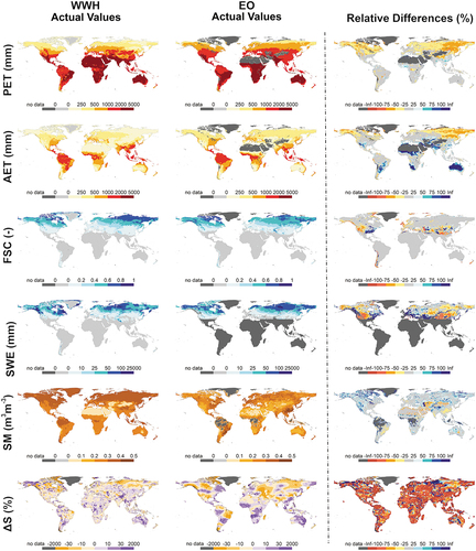
For PET, the general decreasing gradients from the equator to the poles are captured in both datasets. However, when looking into PET relative differences between the two datasets (Fig. 1, row 1, column 3), one can see some local discrepancies. PET results are more similar in the southern hemisphere than in the northern hemisphere. WWH gives lower values of PET in latitudes greater than 30°N with relative differences between −25 and −75%. The different equations used for estimating PET in WWH (Arheimer et al. 2020) and via the EO product (Mu et al. 2011) might be the main reason for this lack of agreement (Pimentel et al. 2023).

In the case of AET, the latitudinal gradients are also well captured in both datasets (Fig. 1, row 2). Again, spatial heterogeneities can be identified in the comparison of the two AET maps. The regions with good agreement between the two analysed data sources (relative differences within the interval from −25 to 25%) are: the Amazonas, central Africa and Indonesia (AET values in the range 1000–2000 mm); eastern North America and central Europe (AET values in the range 500–1000 mm); and western North America, eastern Europe and western Russia (AET values in the range 0–500 mm). In contrast, the regions with lower agreement are southern South America, the Sahel, southern Africa, India, the Mekong region, and Australia. In all these regions AET is estimated up to 75% higher in WWH than in the EO product. The results for eastern Russia and northern Canada also differ, but in this case AET is estimated up to 50% lower in WWH than in the EO product. These differences could be due to systematic errors in the MODIS product, which have been observed in previous studies. When validating the MODIS AET product against other remote sensing products at the global scale, Miralles et al. (2016) highlighted systematic lower values for the MODIS AET product in tropical and sub-tropical regions but larger values in high latitudes of the northern hemisphere.

Snow is distributed similarly worldwide in both WWH and EO products (Fig. 1, rows 3 and 4). In the northern hemisphere, FSC values match well in latitudes between 40°N and 80°N. Values are above 0.4 in both datasets, and relative differences lie within the interval −25 to 25%. However, we also found low agreement in certain areas of this latitude band: the coastal areas of Alaska, Canada, and western Europe. The non-permanent character of snow in these areas, with values of FSC within the interval 0–0.2 (Fig. 1, row 3, columns 1 and 2), leads to drastic relative differences when comparing the two datasets (Fig. 1, row 3, column 3). Greenland and the islands located above 70°N also show low agreement in FSC. The analysis is biased by the limitations of the EO product in capturing snow information during winter months due to the northern nights (Lee et al. 2006, Notarnicola 2020, Rößler et al. 2021). The discrepancy also reflects the different methodologies used for separating ice and snow in WWH (Lindström et al. 2010) versus the EO product (Hall and Riggs 2017). In latitudes between 30° and 40°N, FSC generally shows low agreement between the two data sources. WWH simulates FSC in lower latitudes, where the EO product does not retrieve snow. In the southern hemisphere, the agreement of FSC is low in the Andes and New Zealand, with high relative differences also due to the non-permanent character of snow. The seasonal character of snow in areas with highly seasonal snow (e.g. Sierra Nevada in Spain, Atlas Mountain Range in Morocco, Sierra Nevada in California, Andes in Chile) is not well represented, neither in the WWH model nor in the EO product. Higher resolution, better meteorological data, and/or specific calibration would be needed to capture these local phenomena (Marchane et al. 2015, Cornwell et al. 2016, Pimentel et al. 2017b).

In terms of SWE, the EO product is limited to the northern hemisphere at latitudes above 30°N. This variable shows lower agreement than FSC (Fig. 1, rows 3 and 4, column 3). Relative differences higher than 75% are observed in all regions with data, which indicate low robustness in these estimates. WWH gives lower SWE values than the EO product in Alaska, western North America, and China. In contrast, the EO product provides lower SWE in eastern North America and western Europe. In this case the EO product is not conditioned by the northern night as it operates in the microwave region of the spectrum; however, more uncertainty is introduced due to the major complexity of the retrieval algorithms (Takala et al. 2011).

The long-term mean values of SM in the upper soil layer are more homogeneous in WWH than in the EO product. Nevertheless, both identify the lowest SM values (0–0.1 m³m^–3 in the same areas – the Sahara, Arabian and Gobi deserts – and the highest values (0.2–0.4 m³m⁻³) in latitudes higher than 50°N. When comparing patterns of long-term SM values, extremely dry areas (e.g. Sahara Desert, Arabian Peninsula, Karakum Desert and Gobi Desert) correspond to locations where the WWH model shows much lower values of SM than the EO product, reaching RE values in the interval −50 to −75%. Deserts have also been identified as areas where EO products have low correlation with reanalysis data (e.g. ERA-Interim/Land, Dorigo et al. 2017). Dorigo et al. (2010) attributed these differences to the filling of temporal gaps in the passive microwave time series with lower quality active microwave observations. In contrast, WWH shows larger values than the EO product in a more dispersed fashion across the northern hemisphere without following a clear pattern (e.g. northwestern North America, Siberia, and the Tibetan Plateau). Previous assessments of the EO product have shown poor correlation with in situ measurements in high latitudes, including the high-latitude boreal forest and the Tibetan Plateau (Dorigo et al. 2017).

For ΔS, the results show a general discrepancy between WWH and EO (Fig. 1, row 6, columns 1 and 2). The relative differences show a much lower ΔS in WWH than in the EO product. This difference is almost homogeneous worldwide, with relative differences below −75% for 60% of the global land mass. Small overestimation spots appear dispersedly all over the globe, being significant only in parts of northern Canada and Siberia. This difference might be due to a lack of deep aquifers in these regions, as the WWH model mainly simulates subsurface storage regularly interacting with surface flow (Arheimer et al. 2020). Despite these high differences in ΔS values, the two datasets agree on the sign of ΔS in some regions (i.e. whether the total water storage is increasing – purple in Fig. 3 – or decreasing – orange in Fig. 3). For instance, negative ΔS values in central Canada, the Amazonia and northwestern Siberia, and positive ΔS values in northwestern Canada and Australia, are found in both datasets.

To summarize, global patterns in long-term annual means are similarly represented for PET, AET, FSC and SWE, partly similarly represented for SM and deviate for ΔS when comparing the datasets, i.e. WWH and EO products.

4.2 Seasonal dynamics

Seasonal dynamics were compared using KGE and its components. Regarding evaporation variables, the KGE values for PET point to the regions with similar monthly characteristics in EO and WWH datasets (KGE greater than 0.5; row 1, column 1 in Fig. 2): the eastern USA; the southern part of South America; central, eastern, and southern Europe; southern Africa; and Australia. In these areas, CC, RE and RESD have values close to the optimum. In contrast, northern latitudes (above 50°N), equatorial regions (10°N–10°S), and eastern China show low KGE values (KGE lower than 0.25), due to clear biases in mean and standard deviation (row 1, columns 3 and 4 in Fig. 2). Nevertheless, all regions but the equatorial regions show an agreement in temporal dynamics (based on CC). In the northern latitudes and equatorial regions WWH provides clearly lower values than the EO product (RE and RESD lower than −25%), while in eastern China, WWH has clearly higher values (RE and RESD higher than 25%). These discrepancies could be related to the selection of PET methods in the set-up of the WWH model or to limitations of the MODIS products (Pimentel et al. 2023). For instance, Velpuri et al. (2013) demonstrated that a bias in seasonality was introduced in the MODIS product by the GMAO meteorological data and uncertainty was introduced when filling some gaps for evapotranspiration calculation.

Figure 2. Agreement in monthly dynamics for the study period, 2000–2014, in terms of Kling-Gupta efficiency (KGE) and each of its components: Pearson correlation coefficient (CC), relative error (RE) and relative error of standard deviation (RESD) (columns) for each of the six selected hydrologic variables (rows): potential evapotranspiration (PET), actual evapotranspiration (AET), fractional snow cover (FSC), snow water equivalent (SWE), soil moisture (SM), and changes in water storage (ΔS). High agreement is represented in blue, while low agreement is represented in red (column 1 and 2) yellow and green (column 3 and 4).

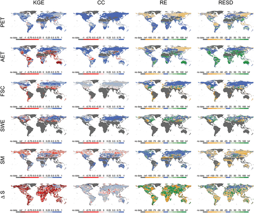
For AET, KGE values are generally lower than for PET, and have different spatial distribution. The largest KGE differences appear in southwestern Canada, the western and some part of central USA, South America, equatorial and southern Africa, the Mediterranean region, central Asia, parts of India, China, the Mekong region and Australia, where the model shows higher values in mean and standard deviation (RE and RESD higher than 25%). Interestingly, these regions generally show a good correlation coefficient (except for the Amazon basin, where CC is lower than 0.25), which indicates that the temporal dynamics of the AET process are well captured but not the magnitude. Low monthly correlation values between EO products and flux tower observations in this region have been reported by Paca et al. (2019). Overall, there is a general tendency to underestimate seasonal AET values in the selected EO product (Michel et al. 2016, Xu et al. 2019, Zhu et al. 2022).

The snow variables, FSC and SWE, show quite similar KGE distributions. They show higher agreement in northern latitudes (above 50°N) than in southern latitudes. The high agreement occurs in regions where snow is permanent during the whole snow season and therefore both the WWH model and EO products can more easily capture snow cycles and their magnitude. However, some spots also present differences in these areas, such as northern Siberia and the Canadian Artic Archipelago for FSC, and some catchments in eastern USA, western Russia, and northern Canada for SWE. Large differences appear in lower latitudes (KGE lower than 0. 5), which could be considered transition zones, where snow dynamics are more changeable within and between years and, consequently, more difficult to capture (Fayad et al. 2017, Pimentel et al. 2017a).

The low KGE values in FSC over these transition regions are combinations of low values in the three KGE components. For instance, monthly correlation is low, with CC values lower than 0.25. The MODIS EO product used for FSC has limitations in capturing timing in these regions, especially the end of the spring melting (Rittger et al. 2013, Yang et al. 2015, Cornwell et al. 2016, Marchane et al. 2017, Pimentel et al. 2017b, Polo et al. 2020). This fact also influences RE and RESD values, with WWH producing lower values and lower deviations than the EO product in western USA, Chile and the Mediterranean Basin (negative RE and RESD) and higher values and higher deviations than the EO product (positive RE and RESD) in eastern USA and parts of the Tibetan Plateau (Fig. 2, row 3, columns 2–4).

Regarding areas with low KGE values for SWE, the correlation between WWH and the EO product is good (CC values higher than 0.75), showing agreement in temporal dynamics. However, WWH gives much higher snow amounts (RE and RESD greater than 75%) than the EO product (positive RE and RESD) in eastern USA and Europe, and lower (RE and RESD lower than −75%) SWE values than the EO product (negative RE and RESD) in middle USA and eastern Asia (row 4, columns 3 and 4 in Fig. 2). These errors could be related to the more complex snow dynamics over these areas not being correctly captured by the model or to the uncertainty associated with a shallow snowpack in the EO product – or to both sources of error. Takala et al. (2011) affirm that the uncertainty in the SWE EO product increases if the snowpack is smaller than 150 mm, which could correspond to shallow snowpacks common over these zones. In any case, the snow variables, and especially FSC due to its low correlation, were found to display lower agreement than PET and AET in terms of seasonal dynamics.

Regarding SM, KGE values show a clear gradient along latitudes in the northern hemisphere. While KGE values above 50°N indicate low agreement (KGE lower than 0), more reasonable values are observed for areas below this latitude (KGE higher than 0.25). This gradient is clearly due to a bad correlation between the two datasets above 50°N, as shown by the patterns in CC (Fig. 2 row 5, column 2) and due to a large difference in RESD, with generally lower SM variability in the model (Fig. 2 row 5, column 4). Dorigo et al. (2017) point out that, in northern latitudes, seasonal gaps due mainly to the presence of dense forests and frozen soils constitute a challenge for retrieving SM from remote sensing. This may be the cause for the mismatch observed in our comparison. However, interestingly, the results observed in terms of the mean bias are very good, with optimum values reached almost worldwide (Fig. 2, row 5, column 3). Exceptions to this good RE are mainly observed in northern Africa and central Asia (RE lower than −0.75) in areas with deserts, which have previously been highlighted as challenging areas (Dorigo et al. 2017). There is a risk that the unclear soil depth representation in the EO product (see Section 2.5) might be shallower and more spatially variable than the first layer of the WWH soil (fixed at 25 cm in this analysis), which thus must be changed to correspond to the EO product.

KGE values for ΔS are globally quite low (KGE lower than 0, for 75% of the total land area covered by GRACE), which means that there is a large discrepancy between the two methods of estimation. Biases in means are larger and differ between regions, being highly skewed one way or the other, also where other researchers have found high correlation between hydrological modelling and this ΔS EO product (e.g. Rakovec et al. 2016, Cáceres et al. 2020). This indicates that the changes in volume might be due to underestimation of aquifers in WWH (see above).

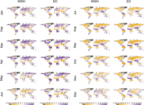
This general mismatch between the two sources is, however, less related to errors in temporal dynamics (CC greater than 0.5, for 53% of the total land area covered by GRACE). We find good agreement in ΔS for March to May (average relative differences between the data sources of 3.6, −2.5 and −21.1% for each month) and discrepancies in February and June to November (mean relative difference between the data sources of 33.5, −39.1, −31.0, −30.9, −42.8, −50.9%, −66.1% for each month) globally (Fig. 3). The biases most negatively affecting the overall agreement in Fig. 1 (row 6) are for December and January (mean relative differences between the data sources of −116.5 and 355.8%). These more extreme discrepancies are found in the northern hemisphere.

Figure 3. Monthly long-term mean of changes in water storages (ΔS) obtained from World-wide HYPE (WWH) (columns 1 and 3) and Earth observation (EO) products from Gravity Recovery and Climate Experiment (GRACE) (columns 2 and 4) for the period 2000–2014.

To summarize, besides PET the seasonal dynamics of the studied variables can be considered robust at the regional scale but not globally. To a large extent this can be referred to uncertainties in the EO products but also to the GHM.

4.3 Hydrological understanding

Here, we evaluate whether the WWH model predicts streamflow for the right reasons, i.e. whether the numerical process descriptions based on our hydrological understanding can be justified from internal model variables. For that, we compared the relationship between (i) the WWH model performance in terms of discharge and (ii) the agreement between EO products and internal WWH model variables (in terms of KGE and its components). We assume that, if the agreement with an EO-product variable is correlated with the WWM model performance in discharge, the representation of the variable in the model may be the cause of the WWH performance in discharge. Alternatively, if they are anti-correlated, the WWH model discharge may be right for the wrong reasons, or wrong for the right reasons.

Hereafter, the analysis is based on 4367 catchments with river discharge information available for the study period (2000–2014). The catchments are divided into four groups using the quantiles of the KGE distribution for WWH model agreement with in situ data from river gauges. Very poor performance is associated with KGE values from −3809.024 to −0.042 (red box plots in Fig. 4); poor performance with values from −0.042 to 0.375 (light red box plots in Fig. 4); acceptable performance with KGE values from 0.375 to 0.634 (light blue box plots in Fig. 4); and very good performance with KGE values from 0.634 to maximum (blue box plots in Fig. 4).

Figure 4. (a) Map of World-wide HYPE (WWH) model performance in terms of river discharges assessed in 4367 catchments with available river discharge observations. These catchments are divided into four groups using the quantiles of the Kling-Gupta efficiency (KGE) distribution for WWH model performance. (b) Agreement of WWH and Earth observation (EO) products in terms of internal hydrologic variables for the period 2000–2014: potential evapotranspiration (PET), actual evapotranspiration (AET), fractional snow cover (FSC), snow water equivalent (SWE), soil moisture (SM), and changes in water storage (ΔS) (y-axis) for each category of WWH flow performance with respect to in situ observations (x-axis). Each column represents a different metric: KGE, Pearson correlation coefficient (CC), relative error (RE) and relative error of standard deviation (RESD). Optimum values are represented by the dashed green line and good performance interval by green area. Note: the 4367 river discharge observation stations were not used in the WWH calibration process.

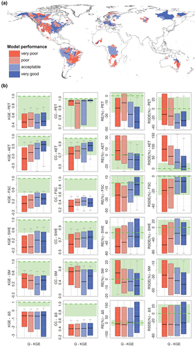
The KGE performances for discharge do not appear to be linked with PET since the four catchment groups show a similar spread in PET agreement and acceptable median values of KGE (around 0.5). The components of the KGE show that even though CC is very high (almost 1) for catchments with high discharge KGE, these catchments are also characterized by substantial negative biases in mean and standard deviation in PET with clearly lower WWH model estimates (median values about −25 and −20%, respectively). These results are in line with the previous conclusions obtained for PET in WWH, suggesting that the spatial selection of the PET models may not be optimal in the model set-up (Pimentel et al. 2023). No clear relation exists between the KGE in discharge and SM either.

Poor similarities in SM are found for KGE (median value about 0.2), because of poor correlation (median CC around 0.6) and a poor RESD (median value about −35%). We see a tendency for poorer SM with improved KGE for discharge, which would indicate that the model is right for the wrong reason, but probably reflects the fact that different soil depths are being compared. Hence, the upper soil layer must be adjusted in upcoming WWH versions, as it is crucial in the interaction between land and atmosphere (Katul et al. 2012) and robustness would be important for analysing societal challenges linked to climate change (Van Loon et al. 2016, Döll et al. 2018, Konapala et al. 2020, Gudmundsson et al. 2021).

ΔS values in the selected catchments show very similar patterns regardless of river flow model performances, with KGE median values of about −0.5, CC about 0.4, RE about 0% in three groups out of four, and RESD about −35%. Therefore, it can be concluded that there is no clear relationship between the performance in discharge, in terms of KGE, and the agreement between WWH and EO estimates for these three analysed variables (PET, SM and ΔS).

However, the results highlight a clear relationship between good performances in modelled discharge and agreement in AET, FSC and SWE. Higher agreement in KGE, CC and RESD in terms of AET is associated with high performances in discharge. Only small mismatches are observed for the median RE, which is within 10% for all four groups. These results indicate that the calibration of the parameters controlling AET in WWH succeeds despite the observed disagreement in PET between EO product and model.

The same relationship is found for FSC, where a higher agreement corresponds to higher KGE values in discharges. Beside snow extent, snow amount seems to follow the same pattern, showing a relation between performances in river discharges and agreement in SWE. A higher agreement in SWE is found when model performance in discharge improves (red box plots for KGE show a median KGE in SWE about −0.05, while blue box plots show a median KGE value in SWE of about 0.2). This could be explained by the location of the catchments, with good-KGE performance in areas with low uncertainties in the SWE provided by the EO products, while catchments with poor performance are located in areas with more ephemeral snowpacks (see above).

To summarize, the results show that AET and the snow variables FSC and SWE are robust variables in the hydrological predictions that improve discharge performance at the global scale, and thus contribute to WWH being right for the right reasons. PET and ΔS, on the other hand, did not influence the model performance in water discharge, while SM may be right for the wrong reasons (but the comparison was biased by soil depths).

5 Conclusions

This work highlights the value of comparing hydrological models at the global scale with various EO products to check the robustness of internal model variables in capturing long-term annual means and seasonal (monthly) patterns to indicate where and when the model is more likely to be “right” for the right reasons.

We propose that hydrological scientists working with scenarios at the global scale should always analyse the model-based robustness to justify their results, either in ensemble modelling of calibrated models (e.g. Krysanova et al. 2017, 2020) or – as in this study – by multi-variable comparison with independent data sources. Preferably, more data sources should be used than in our example; and, ideally, an intergovernmental panel should be established for global water assessments to support policymakers by compiling results from numerous researchers. Only if several sources of data agree should the result be regarded as well supported and to provide credibility when applying GHM results in policy-oriented research on global challenges (e.g. Hoekstra et al. 2012, De Graaf et al. 2019, Rockström et al. 2023). Robustness analysis will also show model limitations and guide model developers regarding where to concentrate their efforts. For instance, the results imply that the current version of WWH should not be applied for analysing deep-groundwater quantities and that results for soil moisture should be treated with caution.

We found that the general patterns of four out of six analysed variables in the hydrological cycle – PET, AET, FSC, and SWE – show similarities between WWH catchment modelling and EO products at the global scale, while a larger discrepancy was found for SM, and very poor agreement for ΔS. Dissimilarities in results indicate that hydrological variables above the ground and earlier in the flow path, such as evaporation and snow, are more robust than the variables describing subsurface downstream processes, such as SM distribution and ΔS. The latter reflects complex processes that can be challenging both to describe with hydrological models and to observe via satellites. The results support previous indications that the WWH model underestimates water in aquifers and thus needs improved representation of groundwater storage. This limits its application in climate change impact studies of future water resources and scenarios for pumping of groundwater reservoirs.

The regional analysis shows that there is little agreement between WWH and EO products in regions with extreme characteristics, such as cold regions (Canadian prairies), arid regions (western USA, deserts), highly forested areas (Amazonas), and transition zones (Sahel and Mediterranean Basin). This indicates that the particularity of these regions calls for specific regional modelling and monitoring approaches rather than continental or global approaches. On the contrary, in some of the temperate regions at mid-latitudes, e.g. eastern USA and central Europe, the long-term mean of the analysed variables (i.e. PET, AET, FSC and SM) showed a reasonable agreement, which means that global approaches can be applied for long-term analysis. For temporal patterns, monthly values of snow variables did not show agreement, which supports previous doubts on quality of the EO products in some snowy regions. We also showed a large discrepancy in terms of SM, indicating that a thinner first layer of soil in the WWH model set-up is probably needed for a higher agreement with EO products.

With respect to equifinality in dynamic model parameters, it is interesting to note that good agreement of AET and snow variables in specific catchments was also linked to good model performance in river discharge at their outlets. This suggests that these processes are comparatively well described in the WWH model. There were no clear indications of good discharge performance associated with bad internal model representation.

Overall, we found the robustness analysis useful, and we recommend the presented approach using EO products combined with in situ river gauges as a standard method in hydrological modelling at the continental or global scale. This approach goes beyond the more traditional evaluation of model performance against river discharges without considering the additional variables from EO products as a ground truth. Hence, the model-based robustness analysis takes advantage of innovative technology and new data without including more uncertainty. This study thus advances UPH No. 16 (Blöschl et al. 2019), by showing the potential and challenge of innovative technologies to measure global heterogeneity of surface and subsurface properties of water state variables and fluxes. This method furthers the identification of caveats in understanding and reproducing the global hydrological cycle in models, without forgetting that EO products also have uncertainties.

Acknowledgements

We would like to thank the Editor and the three anonymous Reviewers of this manuscript (especially Reviewer #2), who have contributed with detailed comments that have helped to obtain an improved version of this work. We would like to also express our gratitude to all EO data providers; without you this study would not have been possible at all. Moreover, we would like to thank the whole SMHI hydrological research unit, where the WWH model has been developed and much of this work was carried out, taking advantage of previous work and several projects running in parallel in the group. Rafael Pimentel acknowledges the funding by the Juan de la Cierva-Incorporación program of the Spanish Ministry of Science and Innovation (IJC2018-038093-I). In addition, RP is currently member of DAUCO, Unit of Excellence ref. CEX2019-000968-M, with financial support from the Spanish Ministry of Science and Innovation, the Spanish State Research Agency, through the Severo Ochoa and María de Maeztu Program for Centers and Units of Excellence in R&D.

Disclosure statement

No potential conflict of interest was reported by the authors.

References

- Alfieri, L., et al., 2023. GloFAS – global ensemble streamflow forecasting and flood early warning. Hydrology and Earth System Sciences, 17 (3), 1161–1175. doi:10.5194/hess-17-1161-2013
- Andersson, J.C.M., et al., 2017. Process refinements improve a hydrological model concept applied to the Niger River basin. Hydrological Processes, 31 (25), 4540–4554. doi:10.1002/hyp.11376
- Archfield, S.A., et al., 2015. Accelerating advances in continental domain hydrologic modeling. Water Resources Research, 51 (12), 10078–10091. doi:10.1002/2015WR017498
- Arheimer, B., et al., 2020. Global catchment modelling using World-Wide HYPE (WWH), open data, and stepwise parameter estimation. Hydrology and Earth System Sciences, 24 (2), 535–559. doi:10.5194/hess-24-535-2020
- Arnell, N.W., 1999. A simple water balance model for the simulation of streamflow over a large geographic domain. Journal of Hydrology, 217 (3–4), 314–335. doi:10.1016/S0022-1694(99)00023-2
- Best, M.J., et al., 2011. The Joint UK Land Environment Simulator (JULES), model description – part 1: energy and water fluxes. Geosciences Model Development, 4 (3), 677–699. doi:10.5194/GMD-4-677-2011
- Beven, K., 2006. A manifesto for the equifinality thesis. Journal of Hydrology, 320 (1), 18–36. doi:10.1016/j.jhydrol.2005.07.007
- Bierkens, M.F.P., et al., 2015. Hyper-resolution global hydrological modelling: what is next? Hydrological Processes, 29 (2), 310–320. doi:10.1002/HYP.10391
- Bierkens, M.F.P., Sutanudjaja, E.H., and Wanders, N., 2021. Large-scale sensitivities of groundwater and surface water to groundwater withdrawal. Hydrology and Earth System Sciences, 25 (11), 5859–5878. doi:10.5194/hess-25-5859-2021
- Blöschl, G., et al., 2019. Twenty-three unsolved problems in hydrology (UPH) – a community perspective. Hydrological Sciences Journal, 64 (10), 1141–1158. doi:10.1080/02626667.2019.1620507
- Cáceres, D., et al., 2020. Assessing global water mass transfers from continents to oceans over the period 1948–2016. Hydrology and Earth System Sicences, 24 (10), 4831–4851. doi:10.5194/HESS-24-4831-2020
- Colwell, R.K., 1974. Predictability, constancy, and contingency of periodic phenomena. Ecology, 55 (5), 1148–1153. doi:10.2307/1940366
- Cornwell, E., Molotch, N.P., and McPhee, J., 2016. Spatio-temporal variability of snow water equivalent in the extra-tropical Andes Cordillera from distributed energy balance modelling and remotely sensed snow cover. Hydrology and Earth System Sciences, 20 (1), 411–430. doi:10.5194/HESS-20-411-2016
- Crochemore, L., et al., 2020. Lessons learnt from checking the quality of openly accessible river flow data worldwide. Hydrological Sciences Journal, 65 (5), 699–711. doi:10.1080/02626667.2019.1659509
- De Graaf, I.E.M., et al., 2019. Environmental flow limits to global groundwater pumping. Nature, 574 (7776), 90–94. doi:10.1038/s41586-019-1594-4
- Demirel, M.C., et al., 2018. Combining satellite data and appropriate objective functions for improved spatial pattern performance of a distributed hydrologic model. Hydrology and Earth System Sciences, 22 (2), 1299–1315. doi:10.5194/hess-22-1299-2018
- Dile, Y.T., et al., 2020. Evaluating satellite-based evapotranspiration estimates for hydrological applications in data-scarce regions: a case in Ethiopia. Science of the Total Environment, 743, 140702. doi:10.1016/J.SCITOTENV.2020.140702
- Döll, P., et al., 2014. Global-scale assessment of groundwater depletion and related groundwater abstractions: combining hydrological modelling with information from well observations and GRACE satellites. Water Resources Research, 50 (7), 5698–5720. doi:10.1002/2014WR015595
- Döll, P., et al., 2018. Risks for the global freshwater system at 1.5 °C and 2 °C global warming. Environmental Research Letters, 13 (4), 044038. doi:10.1088/1748-9326/AAB792
- Döll, P., Kaspar, F., and Lehner, B., 2003. A global hydrological model for deriving water availability indicators: Model tuning and validation. Journal of Hydrology, 270 (1–2), 105–134. doi:10.1016/S0022-1694(02)00283-4
- Donnelly, C., Andersson, J.C.M., and Arheimer, B., 2016. Using flow signatures and catchment similarities to evaluate the E-HYPE multi-basin model across Europe. Hydrological Sciences Journal, 61 (2), 255–273. doi:10.1080/02626667.2015.1027710
- Dorigo, W., et al., 2017. ESA CCI soil moisture for improved earth system understanding: state-of-the art and future directions. Remote Sensing of Environment, 203, 185–215. doi:10.1016/j.rse.2017.07.001
- Dorigo, W.A., et al., 2010. Error characterisation of global active and passive microwave soil moisture datasets. Hydrology and Earth System Sciences, 14 (12), 2605–2616. doi:10.5194/hess-14-2605-2010
- Dozier, J., 1989. Spectral signature of alpine snow cover from the Landsat thematic mapper. Remote Sensing of Environment, 28, 9–22. doi:10.1016/0034-4257(89)90101-6
- Faisol, A., et al., 2020. An evaluation of MODIS global evapotranspiration product (MOD16A2) as terrestrial evapotranspiration in East Java - Indonesia. IOP Conference Series: Earth and Environmental Science, 485 (1), 012002. doi:10.1088/1755-1315/485/1/012002
- Fayad, A., et al., 2017. Snow hydrology in Mediterranean mountain regions: a review. Journal of Hydrology, 551, 374–396. doi:10.1016/j.jhydrol.2017.05.063
- Friedl, M.A., et al., 2002. Global land cover mapping from MODIS: algorithms and early results. Remote Sensing of Environment, 83 (1), 287–302. doi:10.1016/S0034-4257(02)00078-0
- Gädeke, A., et al., 2020. Performance evaluation of global hydrological models in six large Pan-Arctic watersheds. Climate Change, 163 (3), 1329–1351. doi:10.1007/s10584-020-02892-2
- Gascoin, S., et al., 2015. A snow cover climatology for the Pyrenees from MODIS snow products. Hydrology and Earth System Sicences, 19 (5), 2337–2351. doi:10.5194/HESS-19-2337-2015
- GCEW, 2023. The What, Why and how of the world water crisis: global commission on the economics of water phase 1 review and findings. Paris: Global Commission on the Economics of Water.
- Gudmundsson, L., et al., 2021. Globally observed trends in mean and extreme river flow attributed to climate change. Science, 371 (6534), 1159–1162. doi:10.1126/science.aba3996
- Guimberteau, M., et al., 2012. Discharge simulation in the sub-basins of the Amazon using ORCHIDEE forced by new datasets. Hydrology and Earth System Sicences, 16 (3), 911–935. doi:10.5194/HESS-16-911-2012
- Gupta, H.V., et al., 2009. Decomposition of the mean squared error and NSE performance criteria: implications for improving hydrological modelling. Journal of Hydrology, 377 (1), 80–91. doi:10.1016/j.jhydrol.2009.08.003
- Hall, D.K., et al., 2002. MODIS snow-cover products. Remote Sensing of Environment, 83 (1), 181–194. doi:10.1016/S0034-4257(02)00095-0
- Hall, D.K. and Riggs, G.A., 2017. Accuracy assessment of the MODIS snow products. Hydrological Processes, 21 (12), 1534–1547. doi:10.1002/hyp.6715
- Han, P., et al., 2019. Improved understanding of snowmelt runoff from the headwaters of China’s Yangtze River using remotely sensed snow products and hydrological modelling. Remote Sensing of Environment, 224, 44–59. doi:10.1016/J.RSE.2019.01.041
- Han, S.-C., et al., 2005. Improved estimation of terrestrial water storage changes from GRACE. Geophysical Research Letters, 32 (7), 7. doi:10.1029/2005GL022382
- Hancock, S., et al., 2013. Evaluating global snow water equivalent products for testing land surface models. Remote Sensing of Environment, 128, 107–117. doi:10.1016/J.RSE.2012.10.004
- Hargreaves, G.H. and Samani, Z.A., 1982. Estimating Potential Evapotranspiration. Journal of the Irrigation and Drainage Division, 108 (3), 225–230. doi:10.1061/JRCEA4.0001390
- Harrigan, S., et al., 2023. Daily ensemble river discharge reforecasts and real-time forecasts from the operational global flood awareness system. Hydrology and Earth System Sciences, 27 (1), 1–19. doi:10.5194/hess-27-1-2023
- Harris, M. and Frigg, R., 2023. Climate models and robustness analysis – part I: core concepts and premises. In: G. Pellegrino and M. Di Paola, eds. Handbook of Philosophy of Climate Change. Switzerland: Springer Cham. doi:10.1007/978-3-030-16960-2_146-1
- Her, Y. and Chaubey, I., 2015. Impact of the numbers of observations and calibration parameters on equifinality, model performance, and output and parameter uncertainty. Hydrological Processes, 29 (19), 4220–4237. doi:10.1002/hyp.10487
- Hoekstra, A.Y., et al., 2012. Global monthly water scarcity: blue water footprints versus blue water availability. PLoS ONE, 7 (2), e32688. doi:10.1371/journal.pone.0032688
- Hu, G., Jia, L., and Menenti, M., 2015. Comparison of MOD16 and LSA-SAF MSG evapotranspiration products over Europe for 2011. Remote Sensing of Environment, 156, 510–526. doi:10.1016/J.RSE.2014.10.017
- Huang, C., et al., 2018. Detecting, extracting, and monitoring surface water from space using optical sensors: a review. Review of Geophysics, 56 (2), 333–360. doi:10.1029/2018RG000598
- Jensen, M.E. and Haise, H.R., 1963. Estimating evapotranspiration from solar radiation. Proceedings of the American Society of Civil Engineers, Journal of the Irrigation and Drainage Division, 89 (4), 15–41. doi:10.1061/JRCEA4.0000287
- Jin, Y., et al., 2003. Consistency of MODIS surface bidirectional reflectance distribution function and albedo retrievals: 1. Algorithm performance. Journal of Geophysical Research: Atmospheres, 108, D5. doi:10.1029/2002JD002803
- Katul, G.G., et al., 2012. Evapotranspiration: a process driving mass transport and energy exchange in the soil-plant-atmosphere-climate system. Review of Geophysics, 50 (3). doi:10.1029/2011RG000366
- Kim, H.W., et al., 2012. Validation of MODIS 16 global terrestrial evapotranspiration products in various climates and land cover types in Asia. KSCE Journal of Civil Engineering, 16 (2), 229–238. doi:10.1007/s12205-012-0006-1
- Kirchner, J.W., 2006. Getting the right answers for the right reasons: linking measurements, analyses, and models to advance the science of hydrology. Water Resources Research, 42 (3). doi:10.1029/2005WR004362
- Konapala, G., et al., 2020. Climate change will affect global water availability through compounding changes in seasonal precipitation and evaporation. Nature Communication, 11 (1), 3044. doi:10.1038/s41467-020-16757-w
- Krysanova, V., et al., 2017. Intercomparison of regional-scale hydrological models in the present and future climate for 12 large river basins worldwide - A synthesis. Environmental Research Letters, 12 (10), 105002. doi:10.1088/1748-9326/aa8359
- Krysanova, V., et al., 2018. How the performance of hydrological models relates to credibility of projections under climate change. Hydrological Sciences Journal, 63 (5), 696–720. doi:10.1080/02626667.2018.1446214
- Krysanova, V., et al., 2020. How evaluation of global hydrological models can help to improve credibility of river discharge projections under climate change. Climate Change, 163 (3), 1353–1377. doi:10.1007/s10584-020-02840-0
- Landerer, F.W. and Swenson, S.C., 2012. Accuracy of scaled GRACE terrestrial water storage estimates. Water Resources Research, 48 (4), 4. doi:10.1029/2011WR011453
- Lee, T.E., et al., 2006. The NPOESS VIIRS day/night visible sensor. Bulletin American Meteorological Society, 87 (2), 191–200. doi:10.1175/BAMS-87-2-191
- Li, Y., et al., 2018. Hydrologic model calibration using remotely sensed soil moisture and discharge measurements: the impact on predictions at gauged and ungauged locations. Journal of Hydrology, 557, 897–909. doi:10.1016/j.jhydrol.2018.01.013
- Liang, X., et al., 1994. A simple hydrologically based model of land surface water and energy fluxes for general circulation models. Journal of Geophysical Research, 99 (D7), 14415–14428. doi:10.1029/94JD00483
- Lindström, G., et al., 2010. Development and testing of the HYPE (Hydrological Predictions for the Environment) water quality model for different spatial scales. Hydrology Research, 41 (3–4), 295–319. doi:10.2166/nh.2010.007
- Lloyd, E., 2015. Model robustness as a confirmatory virtue: the case of climate science. Studies in History and Philosophy of Science, 49, 58–68. doi:10.1016/j.shpsa.2014.12.002
- Luojus, K., et al., 2016. Assessing global satellite-based snow water equivalent datasets in ESA SnowPEx project. In: 2016 IEEE International Geoscience and Remote Sensing Symposium (IGARSS). Beijing, China, 5284–5287. doi:10.1109/IGARSS.2016.7730376
- Ma, H., et al., 2019. Satellite surface soil moisture from SMAP, SMOS, AMSR2 and ESA CCI: a comprehensive assessment using global ground-based observations. Remote Sensing of Environment, 231, 111215. doi:10.1016/j.rse.2019.111215
- MacDonald, M.K., et al., 2018. Impacts of 1.5 and 2.0 °C warming on Pan-Arctic River discharge into the Hudson Bay complex through 2070. Geophysical Research Letters, 45 (15), 7561–7570. doi:10.1029/2018GL079147
- Marchane, A., et al., 2015. Assessment of daily MODIS snow cover products to monitor snow cover dynamics over the Moroccan Atlas mountain range. Remote Sensing of Environment, 160, 72–86. doi:10.1016/J.RSE.2015.01.002
- Marchane, A., et al., 2017. Climate change impacts on surface water resources in the Rheraya catchment (High Atlas, Morocco). Hydrological Sciences Journal, 62 (6), 979–995. doi:10.1080/02626667.2017.1283042
- Michel, D., et al., 2016. The WACMOS-ET project – part 1: tower-scale evaluation of four remote-sensing-based evapotranspiration algorithms. Hydrology and Earth System Sciences, 20 (2), 803–822. doi:10.5194/hess-20-803-2016
- Miralles, D., et al., 2016. The WACMOS-ET project-part 2: evaluation of global terrestrial evaporation data sets. Hydrology and Earth System Sciences, 20 (2), 823–842. doi:10.5194/hess-20-823-2016
- Montanari, M., et al., 2008. Calibration and sequential updating of a coupled hydrologic-hydraulic model using remote sensing-derived water stages. Hydrology and Earth System Sciences, 5 (6), 3213–3245. doi:10.5194/hessd-5-3213-2008
- Monteith, J.L., 1965. Evaporation and environment. Symposia of the Society for Experimental Biology, 19, 205–234.
- Mortimer, C., et al., 2020. Evaluation of long-term northern hemisphere snow water equivalent products. The Cryosphere, 14 (5), 1579–1594. doi:10.5194/tc-14-1579-2020
- Mu, Q., et al., 2007. Development of a global evapotranspiration algorithm based on MODIS and global meteorology data. Remote Sensing of Environment, 111 (4), 519–536. doi:10.1016/j.rse.2007.04.015
- Mu, Q., Zhao, M., and Running, S.W., 2011. Improvements to a MODIS global terrestrial evapotranspiration algorithm. Remote Sensing of Environment, 115 (8), 1781–1800. doi:10.1016/j.rse.2011.02.019
- Muñoz, E., et al., 2014. Identifiability analysis: towards constrained equifinality and reduced uncertainty in a conceptual model. Hydrological Sciences Journal, 59 (9), 1690–1703. doi:10.1080/02626667.2014.892205
- Myneni, R.B., et al., 2002. Global products of vegetation leaf area and fraction absorbed PAR from year one of MODIS data. Remote Sensing of Environment, 83 (1), 214–231. doi:10.1016/S0034-4257(02)00074-3
- Notarnicola, C., 2020. Hotspots of snow cover changes in global mountain regions over 2000–2018. Remote Sensing of Environment, 243, 111781. doi:10.1016/j.rse.2020.111781
- Notarnicola, C., et al., 2013. Snow cover maps from MODIS images at 250 m resolution, part 2. Validation, 5 (4), 1568–1587. doi:10.3390/rs5041568
- Notarnicola, C., Angiulli, M., and Posa, F., 2008. Soil moisture retrieval from remotely sensed data: neural network approach versus bayesian method. IEEE Transactions on Geoscience and Remote Sensing, 46 (2), 547–557. doi:10.1109/TGRS.2007.909951
- O’Loughlin, R., 2021. Robustness reasoning in climate model comparisons. Studies in History and Philosophy of Science, 85, 34–43. doi:10.1016/j.shpsa.2020.12.005
- Paca, V.H., et al., 2019. The spatial variability of actual evapotranspiration across the Amazon River Basin based on remote sensing products validated with flux towers. Ecological Processes, 8 (1), 1–20. doi:10.1186/s13717-019-0158-8
- Parajka, J., et al., 2012. MODIS snow cover mapping accuracy in a small mountain catchment - Comparison between open and forest sites. Hydrological and Earth System Sciences, 16 (7), 2365–2377. doi:10.5194/HESS-16-2365-2012
- Pechlivanidis, I.G. and Arheimer, B., 2015. Large-scale hydrological modelling by using modified PUB recommendations: the India-HYPE case. Hydrology and Earth System Sciences, 19 (11), 4559–4579. doi:10.5194/hess-19-4559-2015
- Penman, H.L., 1948. Natural evaporation from open water, bare soil, and grass. Proceedings of the Royal Society of London. Series A. Mathematical and Physical Sciences, 193 (1032), 120–145. doi:10.1098/rspa.1948.0037
- Pimentel, R., et al., 2018. Validating improved-MODIS products from spectral mixture-Landsat snow cover maps in a mountain region in southern Spain. PIAHS. doi:10.5194/piahs-380-67-2018
- Pimentel, R., et al., 2023. Which potential evapotranspiration formula to use in hydrological modelling world-wide? Water Resources Research, 59 (5), e2022WR033447. doi:10.1029/2022WR033447
- Pimentel, R., Herrero, J., and Polo, M.J., 2017a. Subgrid parameterization of snow distribution at a Mediterranean site using terrestrial photography. Hydrology and Earth System Sciences, 21 (2), 805–820. doi:10.5194/hess-21-805-2017
- Pimentel, R., Herrero, J., and Polo, M.J., 2017b. Quantifying snow cover distribution in semiarid regions combining satellite and terrestrial imagery. Remote Sensing, 9 (10), 995. doi:10.3390/rs9100995
- Pokhrel, Y.N., Fan, Y., and Miguez-Macho, G., 2014. Potential hydrologic changes in the Amazon by the end of the 21st century and the groundwater buffer. Environmental Research Letters, 9 (8), 84004. doi:10.1088/1748-9326/9/8/084004
- Polo, M.J., et al., 2020. Mountain hydrology in the Mediterranean region, water resources in the Mediterranean region. Elsevier, 51–75. doi:10.1016/B978-0-12-818086-0.00003-0
- Priestley, C.H.B. and Taylor, R.J., 1972. On the assessment of surface heat flux and evaporation using large-scale parameters. Monthly Weather Review, 100 (2), 81–92. doi:10.1175/1520-0493(1972)100<0081:otaosh>2.3.CO;2
- Pulliainen, J.T., Grandell, J., and Hallikainen, M.T., 1999. HUT snow emission model and its applicability to snow water equivalent retrieval. IEEE Transactions on Geoscience and Remote Sensing, 37 (3), 1378–1390. doi:10.1109/36.763302
- Rajib, M.A., Merwade, V., and Yu, Z., 2016. Multi-objective calibration of a hydrologic model using spatially distributed remotely sensed/in-situ soil moisture. Journal of Hydrology, 536, 192–207. doi:10.1016/j.jhydrol.2016.02.037
- Rakovec, O., et al., 2016. Multiscale and multivariate evaluation of water fluxes and states over European River Basins. Journal of Hydrometeorology, 17 (1), 287–307. doi:10.1175/JHM-D-15-0054.1
- Rittger, K., Painter, T.H., and Dozier, J., 2013. Assessment of methods for mapping snow cover from MODIS. Advances in Water Resources, 51, 367–380. doi:10.1016/J.ADVWATRES.2012.03.002
- Rockström, J., et al., 2023. Safe and just earth system boundaries. Nature, 619 (7968), 102–111. doi:10.1038/s41586-023-06083-8
- Rößler, S., et al., 2021. Remote sensing of snow cover variability and its influence on the runoff of Sápmi’s rivers. Geosciences, 11 (3), 130. doi:10.3390/geosciences11030130
- Rost, S., et al., 2008. Agricultural green and blue water consumption and its influence on the global water system. Water Resources Research, 44 (9), 9405. doi:10.1029/2007WR006331
- Ruhoff, A.L., et al., 2013. Assessment of the MODIS global evapotranspiration algorithm using eddy covariance measurements and hydrological modelling in the Rio Grande basin. Hydrological Sciences Journal, 58 (8), 1658–1676. doi:10.1080/02626667.2013.837578
- Salomon, J.G., et al., 2006. Validation of the MODIS bidirectional reflectance distribution function and albedo retrievals using combined observations from the aqua and terra platforms. IEEE Transactions on Geoscience and Remote Sensing, 44 (6), 1555–1565. doi:10.1109/TGRS.2006.871564
- Samuelsson, P., et al., 2011. The Rossby centre regional climate model RCA3: model description and performance. Tellus Atmosphere, 63 (1), 4–23. doi:10.1111/j.1600-0870.2010.00478.x
- Santos, L., Andersson, J.C.M., and Arheimer, B., 2022. Evaluation of parameter sensitivity of a rainfall-runoff model over a global catchment set. Hydrological Sciences Journal, 67 (3), 342–357. doi:10.1080/02626667.2022.2035388
- Schaaf, C.B., et al., 2002. First operational BRDF, albedo nadir reflectance products from MODIS. Remote Sensing of Environment, 83 (1), 135–148. doi:10.1016/S0034-4257(02)00091-3
- Schupbach, J.N., 2018. Robustness analysis as explanatory reasoning. The British Journal for the Philosophy of Science, 69 (1), 275–300. doi:10.1093/bjps/axw008
- Sood, A. and Smakhtin, V., 2015. Global hydrological models: a review. Hydrological Sciences Journal, 60 (4), 549–565. doi:10.1080/02626667.2014.950580
- Takala, M., et al., 2011. Estimating northern hemisphere snow water equivalent for climate research through assimilation of space-borne radiometer data and ground-based measurements. Remote Sensing of Environment, 115 (12), 3517–3529. doi:10.1016/j.rse.2011.08.014
- Tang, Q., et al., 2007. The influence of precipitation variability and partial irrigation within grid cells on a hydrological simulation. Journal of Hydrometeorology, 8 (3), 499–512. doi:10.1175/JHM589.1
- Thornthwaite, C.W., 1948. An approach toward a rational classification of climate. Geographical Review, 38 (1), 55–94. doi:10.2307/210739
- Van Loon, A.F., et al., 2016. Drought in a human-modified world: reframing drought definitions, understanding, and analysis approaches. Hydrology and Earth System Sciences, 20 (9), 3631–3650. doi:10.5194/hess-20-3631-2016
- Velpuri, N.M., et al., 2013. A comprehensive evaluation of two MODIS evapotranspiration products over the conterminous United States: using point and gridded FLUXNET and water balance ET. Remote Sensing of Environment, 1 (39), 35–49. doi:10.1016/j.rse.2013.07.013
- Vörösmarty, C.J., et al., 2000. Global water resources: vulnerability from climate change and population growth. Science, 289 (5477), 284–288. doi:10.1126/science.289.5477.284
- Wada, Y., Wisser, D., and Bierkens, M.F., 2014. Global modeling of widthdrawal, allocation and consumptive use of surface water and groundwater resources. Earth System Dynamics, 5 (1), 15–40. doi:10.5194/esd-5-15-2014
- Wahr, J., Molenaar, M., and Bryan, F., 1998. Time variability of the earth’s gravity field: hydrological and oceanic effects and their possible detection using GRACE. Journal of Geophysical Research: Solid Earth, 103 (B12), 30205–30229. doi:10.1029/98JB02844
- Widén-Nilsson, E., Halldin, S., and Xu, C., 2007. Global water-balance modelling with WASMOD-M: parameter estimation and regionalisation. Journal of Hydrology, 340 (1), 105–118. doi:10.1016/j.jhydrol.2007.04.002
- Wigneron, J.-P., et al., 2017. Modelling the passive microwave signature from land surfaces: a review of recent results and application to the L-band SMOS & SMAP soil moisture retrieval algorithms. Remote Sensing of Environment, 192, 238–262. doi:10.1016/j.rse.2017.01.024
- Xu, T., et al., 2019. Evaluation of twelve evapotranspiration products from machine learning, remote sensing, and land surface models over conterminous United States. Journal of Hydrology, 578, 124105. doi:10.1016/J.JHYDROL.2019.124105
- Xu, X., Li, J., and Tolson, B.A., 2014. Progress in integrating remote sensing data and hydrologic modelling. Progress in Physical. Geography: Earth and Environment, 38 (4), 464–498. doi:10.1177/0309133314536583
- Yang, J., et al., 2015. Evaluation of snow products over the Tibetan Plateau. Hydrological Processes, 29 (15), 3247–3260. doi:10.1002/HYP.10427
- Zeng, J., et al., 2015. Evaluation of remotely sensed and reanalysis soil moisture products over the Tibetan Plateau using in situ observations. Remote Sensing of Environment, 163, 91–110. doi:10.1016/j.rse.2015.03.008
- Zhu, W., et al., 2022. Multi-scale evaluation of global evapotranspiration products derived from remote sensing images: accuracy and uncertainty. Journal of Hydrology, 611, 127982. doi:10.1016/J.JHYDROL.2022.127982