Gauging the ungauged: estimating rainfall in a West African urbanized river basin using ground-based and spaceborne sensors

ABSTRACT

Accurate precipitation observations are crucial for hydrological forecasts, notably over rapidly responding urban areas. This study evaluated the accuracy of three gridded spaceborne rainfall products (Integrated Multi-satellitE Retrievals for GPM (IMERG), Meteosat Second Generation Visible (MSG-VIS), and MSG-Infrared (MSG-IR)) and the non-governmental Trans-African Hydro-Meteorological Observatory (TAHMO) gauges across the Odaw catchment (Accra, Ghana) from January 2020-July 2022. IMERG is hardly able to capture the strong spatial variability of rainfall required for flood forecasting, but agrees in annual sums with TAHMO and MSG-IR. MSG-IR has difficulties during the wet season. MSG-VIS, only available during daylight, shows limited accuracy and gives high estimates while other products do not detect rain. TAHMO gauges effectively record high-intensity events and their strong spatial variability, although some (daily) accumulations are doubtful and data gaps exist due to technical issues. These findings assist hydrological modelers in selecting appropriate datasets at suitable spatiotemporal resolutions for their research.

KEYWORDS:

• precipitation
• floods
• Accra
• raingauges
• satellite measurements

Editor A. Castellarin; Associate Editor F. Tauro

1 Introduction

The water cycle is expected to intensify as a consequence of global warming (Held and Soden 2006, Hirmas et al. 2018, Yu et al. 2020). Subsequently, rainfall events are projected to become more intense (Wentz et al. 2007, Burt et al. 2016). The risk of pluvial flooding is therefore expected to increase in many parts of the world. Pluvial flooding is especially relevant in urban areas, where impenetrable, paved surfaces result in lower infiltration capacity and even shorter hydrological response times to extreme rainfall events than in rural or natural areas (Johnson et al. 2016, Cristiano et al. 2017). Urban floods are identified as one of the major challenges society will face in the 21st century because of their increasing probability of occurrence and their potentially severe consequences (Gasper et al. 2011, Jha et al. 2012, Pörtner et al. 2022, van Hateren et al. 2023).

Additional flood risk in urban areas is caused by the accumulation of natural and plastic debris within urban drainage systems (Roebroek et al. 2021), which may result in the blockage of those drainage systems (Honingh et al. 2020). High-resolution models that are able to simulate hydrology, hydrodynamics, and debris transport through urban catchments are required for accurate forecasting and protection against floods. These high-resolution models need accurate forcing data for realistic outcomes (Lobligeois et al. 2014). Rainfall represents the main input of such models, requiring accurate observations at high spatial and temporal resolutions due to its strong spatiotemporal variability and the sensitivity of the hydrological system to this variability (Rudolf et al. 1994, Chaubey et al. 1999, Berne et al. 2004, Chambon et al. 2013, Paschalis et al. 2014).

Because of its urgency and significant social and economic impact, the study of (extreme) precipitation data in urban areas is a rapidly developing field of research (Chen and Chandrasekar 2015, Ochoa-Rodriguez et al. 2015, Rios Gaona et al. 2017, Cifelli et al. 2018, de Vos et al. 2018). The majority of such studies have focused on Europe and the United States thanks to the availability of reliable precipitation measurements for these areas. “Traditional” ground-based measurements, such as those from weather radar and raingauges, are accurate but do not cover substantial parts of Africa, Asia, and Southern America (Lorenz and Kunstmann 2012, Saltikoff et al. 2019). At the same time, these areas suffer from extreme precipitation events and floods with a large societal, economic, and environmental impact (Jonkman 2005, Douben 2006, Douglas et al. 2008, Mirza 2011, Tellman et al. 2021, Clarke et al. 2022).

The Odaw catchment (270 km²) in Accra, the capital of Ghana, is a densely populated area vulnerable to pluvial floods resulting from extreme precipitation. During the past three decades Accra has been challenged with floods (Smith 2015, Ackom et al. 2020), and an estimated 30% of residents live in areas vulnerable to (the impact of) floods (Marinetti et al. 2016). Furthermore, plastic debris blocking the drainage system in Accra is a major concern (Tulashie et al. 2020, Dasgupta et al. 2022), resulting in increased flood risk. As explained before, this relationship can only be explored with hydrological models requiring high-resolution precipitation estimates. Although the spatial variability of precipitation over the Odaw catchment has been investigated using raingauges of the Ghana Meteorological Agency (Ackom et al. 2020), the number of official raingauges was limited to three.

Here, we analyse four non-traditional precipitation datasets over the Odaw catchment in Ghana. This can be seen as a first step to increase our understanding of the interaction between (extreme) precipitation and floods in urban catchments that also suffer from plastic debris accumulation (Pinto et al. 2023). Precipitation estimates retrieved from satellites and non-governmental low-cost raingauges are used. The aim of this study is not to validate the satellite rainfall observations as such. Instead, the results of this study will assist future hydrological modellers in their choice of a non-traditional observation that best fits the aim of their study. Additionally, this study provides insights into the precipitation dynamics within the Odaw catchment.

2 Methods and data

2.1 Study site

The Odaw drainage basin is located in the Greater Accra region in the south of Ghana (Fig. 1). The Odaw catchment lies within the most urbanized and densely populated area in this region. The catchment covers an area of 270 km² and drains the major urbanized areas of Accra (Larmie 2019).

Figure 1. Location of the Odaw River basin (black outline) with locations of TAHMO stations (red dots), the channel network (blue), and population density within a district (colour scale). The population density is highest in the downstream part of the catchment and close to the coast. At least one TAHMO station is situated in each district. The dashed line at 5.7°N indicates the boundary used in this study to divide the catchment into the upstream (north of the line) versus downstream (south of the line) parts.

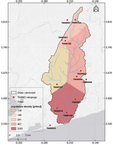
The southern part of Ghana has two rainy seasons: the major one from April to the beginning of July and the minor one from September to the end of October (Manzanas et al. 2014). The average annual rainfall in the basin is 730 mm (Larmie 2019). Rain events over the catchment are often short but intense, occasionally resulting in local flooding (Amoako and Frimpong Boamah 2015, Andreasen et al. 2022).

2.2 Study period

The study was conducted from January 2020 until July 2022. Furthermore, three days with reported floods, which were selected using Lexis Nexis (an online archive with newspapers varying in scope from local to international), were studied in more detail. The three flood events – 9 June 2020 (Tarlue 2020a), 10 October 2020 (Tarlue 2020b), and 21 May 2022 (Okertchiri 2022) – were selected because they all occurred after heavy rainfall and were reported to have a large social impact such as destruction of houses, blocked roads, and even multiple deaths.

2.3 Data

The specifications of the datasets used in this study are presented in Table 1. Many other spaceborne precipitation products exist, such as Precipitation Estimation from Remotely Sensed Information using Artificial Neural Networks (PERSIANN) (Nguyen et al. 2018), CPC MORPHing technique (CMORPH) (Wu 2018), Climate Hazards Group InfraRed Precipitation with Station data (CHIRPS) (Funk et al. 2015), and Global Satellite Mapping of Precipitation (GSMaP) (Kubota et al. 2020). The three satellite products employed in this study were selected because of their high temporal resolution (30 min or higher), their availability over the studied area and during the studied period, and because the products are based on different types of orbits. Two of the evaluated products are based on observations retrieved from geostationary satellites. One of the two is based on all channels, resulting in limited temporal availability, while the other product is based on only infrared (IR) channels, resulting in a continuous availability. The third product Integrated Multi-satellitE Retrievals for GPM (IMERG) is a merged product based on polar orbiting satellites. Each dataset is briefly discussed in the following subsections.

Table 1. The characteristics of the four rainfall products used in this study. These four products are: Meteosat Second Generation Infrared (MSG-IR), Meteosat Second Generation Visible (MSG-VIS), Integrated Multi-satellitE Retrievals for GPM (IMERG), and the non-governmental Trans-African Hydro-Meteorological Observatory (TAHMO) rain gauges.

Name	MSG-IR	MSG-VIS	IMERG	TAHMO
Spatial resolution	3 km × 3 km	3 km × 3 km	10 km × 10 km	Point
Time resolution	15 min	15 min	30 min	15 min
Availability	Continuous	Daytime	Continuous	Continuous
Point vs pixel	Pixel	Pixel	Pixel	Point
Remote vs in situ	Space	Space	Space	Ground

2.3.1 Ground-based rainfall estimates: TAHMO gauge network

The number of gauges maintained by the Ghana Meteorological Agency in the study area is limited and the highest available time resolution is daily. However, the presented research purposes require a higher resolution. The Trans-African Hydro-Meteorological Observatory (TAHMO) operates raingauges across Sub-Saharan Africa (van de Giesen et al. 2014) with a temporal resolution of 15 min and a latency of 1 h. In total, 12 TAHMO stations, all equipped with ATMOS 41 Sensors electronic drop-counting gauges (K. Duah, personal communication, February 2023; METER Group 2021), were selected. Nine of these stations are located within the catchment. The other three are within 5 km of the catchment. The locations of the TAHMO stations are shown in Fig. 1 and summarized in the Appendix (Table A1). Three stations were not available during the studied rainfall period: TA00691 (not available before 2020), TA00314 (defunct for a large part of 2020), and TA00652 (defunct since 14 May 2022).

2.3.2 Space-based rainfall estimates from combined sources: IMERG-L V06B

This study used the most recent version (V06B) of the gridded precipitation product from the Global Precipitation Measurement mission (GPM): the Integrated Multi-satellitE Retrievals for GPM (IMERG) (Huffman et al. 2019). IMERG combines radiometer observations from a constellation of various low earth orbit (LEO) satellites. In case the time between two subsequent satellite overpasses over a certain location is more than 30 min, the most recent observation is morphed forward in time with help of motion vectors calculated from reanalysis data (Modern-Era Retrospective Analysis for Research and Applications, version 2 (MERRA-2) or Goddard Earth Observing System Forward Processing (GEOS-FP), depending on the latency of the IMERG product). Combining and morphing yields a global precipitation product with continuous coverage in both space and time (characteristics can be found in Table 1). More information about IMERG is provided in Tan et al. (2019), Huffman et al. (2020), and references therein.

IMERG is available in the form of two near-real-time (NRT) products (Early, IMERG-E and Late, IMERG-L) and one post-real-time product (Final, IMERG-F). IMERG-F has a higher accuracy than the two NRT runs due to monthly corrections based on raingauges of the Global Precipitation Climatology Centre (GPCC) (Huffman et al. 2019, Tapiador et al. 2019, Hosseini-Moghari and Tang 2020, Li et al. 2021). The effect of these raingauge adjustments is largest over densely gauged areas, while Ghana is largely ungauged. Additionally, monthly adjustments might not be sufficient for the precipitation variability within this area (Echeta et al. 2022). Furthermore, IMERG-F only becomes available after a couple of months due to this inclusion of the raingauges, while the latency is reduced to 4 h and 14 h for IMERG-E and IMERG-L, respectively.

The aforementioned studies also revealed that IMERG-L outperforms IMERG-E. This is attributed to (1) the inclusion of additional data that is not available within the latency of IMERG-E and (2) the propagation of observations both forward and backward in time in IMERG-L, while IMERG-E only comprises forward extrapolation. Hence, IMERG-L is selected for this study because of the combination of higher accuracy compared to IMERG-E, the presumably limited effect of the GPCC gauge correction over Accra, and the shorter latency compared to IMERG-F. The IMERG-L V06B product is referred to as IMERG in the remainder of this paper.

2.3.3 Space-based rainfall estimates from geostationary satellites: MSG-SEVIRI

The Meteosat Second Generation (MSG) is a series of geostationary satellites. Each satellite carries the Spinning Enhanced Visible (VIS) and InfraRed (IR) Imager (SEVIRI) aboard, an imager with 12 narrow-band channels in the VIS to IR spectral range. The Royal Netherlands Meteorological Institute (KNMI) has developed two algorithms to estimate precipitation from SEVIRI observations. Both algorithms were used in this study and are briefly described below.

The Cloud Physical Properties (CPP) algorithm is used to retrieve cloud optical thickness, particle size, and condensed water path from SEVIRI VIS and near-IR observations. These cloud properties are derived for satellite pixels identified as cloudy and based on the thermodynamic phase (liquid or ice). A more extensive description of the algorithm and determination of the thermodynamic phase is provided in Benas et al. (2017). As a next step, the cloud properties are converted to precipitation rates using an empirical approach outlined by Roebeling et al. (2012) and Roebeling and Holleman (2009). This precipitation product is only available during daytime (for solar zenith angles below 84°) since it requires measurements of reflected sunlight. The CPP product is referred to as MSG-VIS in the remainder of this paper.

The Night-time IR Precipitation Estimation (NIPE) algorithm uses brightness temperatures measured by the individual MSG-SEVIRI IR channels as well as brightness temperature differences between channels to estimate precipitation rates. The retrieval relies on relations established between SEVIRI IR measurements and precipitation observations from an independent spaceborne radar (the same radar that is used within GPM). These relations are a function of cloud type. Detailed information about the NIPE algorithm is given by Brasjen and Meirink (2015). Since NIPE uses only IR channels, it can be applied during day and night. The product is referred to as MSG-IR in the remainder of this paper.

2.4 Data pre-processing

To directly compare the four different precipitation products, we performed spatiotemporal matching. The temporal matching was straightforward: two subsequent time steps of MSG and TAHMO were averaged to match IMERG’s 30 min resolution. All time references within this paper are in UTC, but it should be noted that UTC and Local Standard Time (LST) are the same in Ghana. The spatial matching was done using a nearest-neighbour approach, by allocating TAHMO stations to the pixel (either IMERG or MSG) with the shortest distance from the pixel centre. In case two or more TAHMO stations were allocated to one pixel, their arithmetic mean was used. MSG pixels were spatially averaged to the IMERG resolution. When focusing on individual TAHMO stations, the pixel closest to the station was selected. As the spatial resolution of IMERG is coarser than that of MSG, an IMERG pixel is more likely than an MSG pixel to comprise a TAHMO raingauge. Hence, in addition to the MSG product at its native resolution, the MSG product resampled to IMERG resolution was included in the analysis. The number of pixels and the percentage exceeding the wet/dry threshold are shown in the Appendix (Table A2). All MSG pixels and TAHMO stations that fall within the eight selected IMERG pixels are used to calculate the spatial average.

3 Results

3.1 Daily and annual rainfall cycles

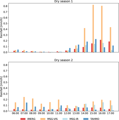
First, the daily and seasonal cycles of rainfall over the Odaw catchment and the ability of the different rainfall products to capture these cycles are discussed. Fig. 2 shows the average daily cycle based on TAHMO, IMERG, MSG-IR, and MSG-VIS, for the dry (November–March, July–August) and wet (April–June, September–October) seasons. The estimates from MSG-VIS during the dry season are higher compared to the other three products, especially between 2.00pm and 6.00pm, when the estimates are 4–5 times higher compared to the other products. When the dry season is divided into two parts (first dry season: November, December, January, February; second dry season: July, August), it is evident the overestimation occurs particularly during the first dry season (Fig. A1).

Figure 2. Spatially and temporally averaged daily cycle of precipitation according to TAHMO, IMERG, MSG-IR and MSG-VIS. The spatial average is based on all MSG pixels and TAHMO stations that fall within an IMERG pixel. (a) Dry season; (b) wet season. All observations, i.e. both wet and dry moments, are included. The x-axis ticks indicate the beginning of each time interval.

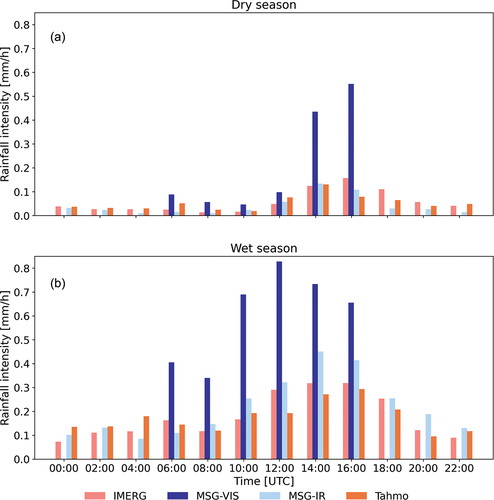
The dependency of MSG-VIS on daylight hours is especially limiting during the wet season (Table 2). About 35–50% of the rainfall events are at night during this season, so MSG-VIS is expected to miss a considerable share of the rain. The percentage of rain during the night decreases with increasing threshold (the threshold was varied from 0.1 to 5 mm/h; not shown). However, even when implementing a threshold of 5 mm/h, the three products have a minimum rainfall fraction of 30% during the night. MSG-IR has the largest day/night difference among the three continuously available products, especially during the wet season.

Table 2. Distribution of observations exceeding the threshold of 0.1 mm/h over daytime and night-time for three of the considered products (expressed as percentages).

	Dry season		Wet season
	Day	Night	Day	Night
IMERG	53	47	55	45
TAHMO	52	48	53	47
MSG-IR	58	42	62	37

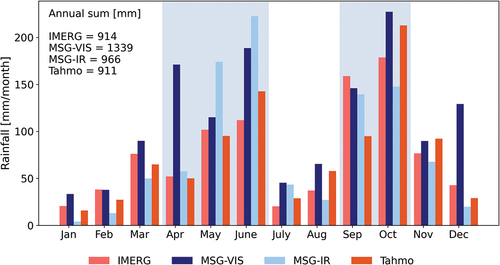
Fig. 3 shows that IMERG, MSG-IR, and TAHMO are able to capture the wet and dry seasons. MSG-IR gives higher rainfall amounts, especially in May and June (respectively 174 mm and 222 mm, about 1.5 times higher than TAHMO and IMERG). MSG-VIS is less capable of distinguishing the different seasons. In general, estimates retrieved from MSG-VIS are much higher than those from the other three products, despite the product being only available during daylight. During April (begin wet season) and December (dry season), MSG-VIS estimates are more than 3 times higher compared to the other three products.

Figure 3. Spatially averaged monthly rainfall accumulations according to TAHMO, IMERG, MSG-IR and MSG-VIS for 2020 and 2021 (2022 is removed because only the first half of the year is covered within the research period). MSG-VIS estimates are based on daytime only: all values during the night are set to 0 mm/month. The blue areas correspond to the wet season.

3.2 Spatial rainfall variation

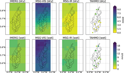
The differences between MSG-VIS and the other products are even more apparent when evaluating the spatial variation of the seasonally averaged precipitation (Fig. 4). Although MSG-VIS is able to capture the north–south gradient of rainfall within the catchment during the dry season (the farther north, the wetter the catchment), its estimates are high compared to the other products. During the dry season, the discrepancy is especially large in the north of the catchment. MSG-VIS gives around 10 mm/d in the north, while the other products give a maximum of 3 mm/d. During the wet season, MSG-VIS estimates are twice as high as the other products. All products are able to capture the spatial variation in the dry season and the reduced spatial gradient in the wet season.

Figure 4. Seasonally averaged precipitation estimates for the entire study period (January 2020–July 2022), distinguishing dry season (upper panels) and wet season (lower panels). Note that the colour bar is season dependent.

3.3 Probability distribution of rainfall intensities

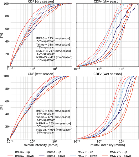
Fig. 5 shows the cumulative distribution functions of the occurrence of rainfall intensities (CDF, left panels) and of their contribution to the total rainfall volume (CDF_v, right panels). The estimates are spatially averaged over the upstream (north of 5.7°N, black dashed line in Fig. 1) or downstream (south of 5.7°N) part of the catchment. The difference between upstream and downstream, both in terms of occurrence and in terms of rainfall sums, is most apparent during the dry season. During this season, IMERG seems biased towards lower rainfall intensities: 40% of rainfall observed by IMERG has an intensity above 0.4 mm/h, while for the other products at least 55% has an intensity above 0.4 mm/h. IMERG attributes 55% of the total precipitation during the dry season to the upstream part of the catchment, compared to 73% according to TAHMO. Yet IMERG can capture the difference in rainfall intensity during the wet and dry season. The highest intensities and sums are provided by MSG-VIS: 471 mm during the dry season and 996 mm during the wet season, almost 1.5 times higher than the sums observed by the other three products.

Figure 5. Cumulative distribution functions of rainfall occurrence (CDF; left) and volume (CDF_v; right) for the entire study period (January 2020–July 2022). All products are spatially averaged over the upstream (north of 5.7°N, dashed lines) or downstream (south of 5.7°N, solid lines) area of the catchment. Only spatially averaged estimates exceeding the dry/wet threshold (1 mm/h) are included. The CDFs are calculated with a logarithmically spaced bin width. Note that the rainy season consists of five months, while the dry season consists of the other seven months.

3.4 Detection of high rainfall intensities

From all TAHMO observations with a minimum 30 min rainfall intensity of 0.1 mm/h, the 5% highest rainfall intensities were selected. Estimates from the other products were matched to the selected TAHMO observations. The corresponding rainfall intensities are shown in Fig. 6 (upper panels). While 50% of the selected TAHMO intervals corresponds to more than 15 mm/30 min of rain, MSG-IR and IMERG do not even retrieve rainfall sums above 15 mm/30 min. In this respect, MSG-VIS is in better correspondence with TAHMO. However, the suitability of MSG-VIS in relation to flooding remains limited as a significant amount of intense rain occurs during the night. When reducing the temporal resolution and focusing on 3 h time intervals, the differences become even more apparent (Fig. 6, lower panels). MSG-IR and IMERG do not provide rainfall sums exceeding 80 mm/3 h, while according to TAHMO and MSG-VIS 80 mm/3 h corresponds to 90% or 30%, respectively, of the total volume. The difference between MSG at IMERG or native resolution shows that, as expected, the occurrence and contribution of high intensities decreases with resolution. For instance, MSG-VIS at native resolution gives intensities up to 130 mm/3 h, while MSG-VIS at IMERG resolution does not yield sums higher than 90 mm/3 h.

Figure 6. Cumulative distribution functions of rainfall occurrence (CDF; left) and volume (CDF_v; right) of the 5% highest rainfall sums in 30 min (upper) and 3 h (lower) time intervals. Selection of time intervals is based on TAHMO observations corresponding to non-exceedance probabilities of 95–100%. For comparison, MSG is resampled to the IMERG grid (labeled with [IM]) to show the effect of resolution (dashed lines). CDFs are calculated with a 2 mm bin width. The total number of TAHMO observations (n) is shown in the lower right corner of each graph.

3.5 Case studies

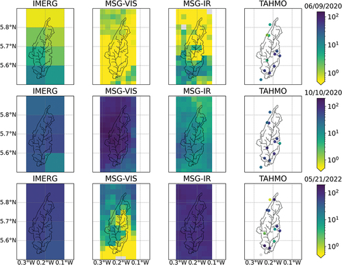
The spatial distributions of daily sums during three selected case studies are shown in Fig. 7. In case 1 (6 June 2020), a precipitation system entered the catchment in the north in the late evening of 5 June. The event moved in a southward direction and crossed the catchment in 5 h. Case 2 (10 October 2020) was a longer rainfall event over the entire catchment. It started in the early morning and lasted until the afternoon. Case 3 (5 May 2022) moved from the north to the south of the catchment in 3 h. In the south, intensities up to 120 mm/h were measured by TAHMO (after sunset, explaining the low sums measured by MSG-VIS).

Figure 7. Daily rainfall sums according to the four products during three case studies. Each row depicts one case. Yellow represents pixels that fall below the lower threshold. Grey represents dry pixels/points.

Fig. 8 shows that both MSG products have a large range of observed rainfall intensities, which is in agreement with Fig. 5 and highlights the high space-time variability of rainfall. The range indicated by the whiskers is smallest for IMERG for all cases and largest for the MSG products. This can be partly attributed to MSG’s higher spatial resolution (resulting in less smoothing) compared to IMERG. IMERG’s coarser resolution reduces the observed precipitation variability. To demonstrate this, the MSG estimates resampled to IMERG resolution are also included. The range between the whiskers in case 1 decreases from 0.15–6 mm/h to 0.18–3 mm/h when resampling MSG-IR to IMERG resolution. IMERG and MSG-IR (native resolution) do not capture the high rainfall intensities during case 1: the 95th percentile is 2 mm/h according to IMERG, while it is 35 mm/h according to TAHMO. Both IMERG and MSG-IR do, however, detect higher intensities for the other two cases. IMERG especially detects the intense rates for case 3. Yet its 95th percentile is an intensity of 20 mm/h while the 95th percentiles of the other products range from 30 to 60 mm/h. The overestimation of MSG-VIS products, discussed earlier in the Results (subsection 3.1), seems limited, but this can be attributed at least partly to the fact that cases 1 and 3 occur largely during night-time hours.

Figure 8. Box plots for each case study for the relevant time interval (case 1: 12.00am to 7.00am, case 2: 3.00am to 1.00pm, case 3: 4.00pm to 10.00pm). All pixels and stations within an IMERG pixel are included. The whiskers correspond to the 5th and 95th data percentiles, the boxes to the 25th and 75th percentiles. The black line represents the median, the green triangle the mean. Case 1 for the MSG-VIS at IMERG resolution (MSG-VIS[IM]) is not shown due to the limited number of data points. Note the y-axis is logarithmic. Rainfall intensities are measured over a 30 min time interval.

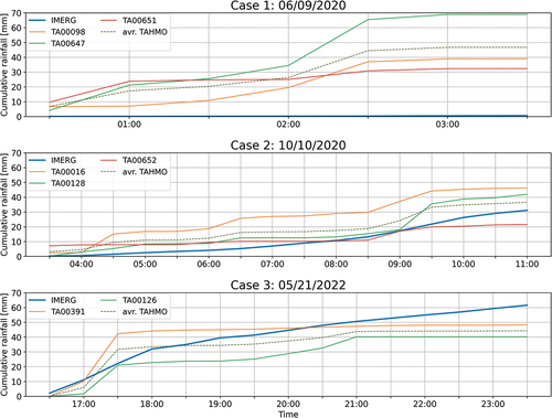
Finally, Fig. 9 shows example time series for one IMERG pixel and the available TAHMO stations within that pixel for the three selected cases. Hence, it shows the rainfall variability within one IMERG pixel. The first case is completely missed by IMERG (pixel with centre 0.15°W, 5.65°N). For the second case, IMERG’s estimates are much smoother than TAHMO. The total amount at the end of the time interval, however, seems correct. In the last case, although the two stations are within one IMERG pixel, the timing of the event is different for each station. This illustrates the limitation of both IMERG and a limited gauge network to represent spatial and temporal rainfall variability.

Figure 9. Comparison of precipitation time series from IMERG and TAHMO for the three considered events. One IMERG pixel and the various stations within that pixel are plotted for each case study. The dashed line represents the average of the selected TAHMO stations. The time interval varies per case study.

4 Discussion

Monthly, seasonal, and annual precipitation accumulations of TAHMO and IMERG are found to be comparable (annual estimates of 910 mm). MSG-IR reports drier dry seasons (namely 214 mm, compared to 295 mm according to IMERG and 338 mm compared to TAHMO) and wetter wet seasons (namely 765 mm, compared to 675 mm according to IMERG and 669 mm according to TAHMO). MSG-VIS greatly overestimates precipitation accumulations, despite its limited availability (only during daylight hours). All products provide higher annual accumulations (Fig. 3) than the estimate of 730 mm (Larmie 2019) mentioned in section 2.1. However, the characteristics of the input data used by Larmie (2019), such as observation method and studied year, are unknown. The studied year(s) can greatly affect the (averaged) yearly total. For instance, the rainfall accumulation of 2020 and 2021 already differed by at least 120 mm, depending on the product (not shown). Furthermore, other studies focusing on floods showed that the annual rainfall estimates over the Odaw catchment can vary between 700 and 1200 mm (e.g. Amoako and Frimpong Boamah 2015, Ackom et al. 2020). Even compared to this range, MSG-VIS observations for the study period are unrealistically high, as its average annual sum is 1339 mm (Fig. 3).

IMERG is able to correctly capture daily rainfall sums, in agreement with other validation studies in this area (Dezfuli et al. 2017, Echeta et al. 2022). MSG-VIS overestimates the amount of rainfall, especially during the dry season in the afternoon. This overestimation is particularly present during November, December, January, and February (Fig. A1(a)), while it is absent in July and August (Fig. A1(b)). A possible source of error might be related to evaporation below the cloud base. Although MSG-VIS may correctly identify clouds as precipitating, it cannot observe whether the precipitation actually reaches the ground surface or whether it has evaporated along the way (Dinku et al. 2011, Hobouchian et al. 2017). Additionally, several other sources of error may play a role due to the indirect retrieval of precipitation via sensors based on geostationary satellites (Bennartz et al. 2010).

Evaporation of precipitation before reaching the ground might be stronger in the first dry period, when a phenomenon called “Harmattan dust” occurs over Ghana. The Harmattan dust is a very dry and dust-laden wind that blows at 3 km height (Breuning-Madsen and Awadzi 2005, He et al. 2007). Since the air (and surface) is very dry, evaporation below the cloud-base might be more apparent in the first dry season compared to the second dry season. An additional source of error might be the incorrect classification of the Harmattan dust as clouds. However, in that case we would expect a larger precipitation area, while the precipitation areas considered in this study appeared to be more convective (not shown). Additionally, the MSG-VIS algorithm is tuned on the Dutch weather radars. This may lead to the false identification of rain due to climatological differences.

In general, IMERG provides the lowest rainfall intensities, followed by MSG-IR, TAHMO, and MSG-VIS measuring the highest intensities (Fig. 6). The high estimates observed from MSG-VIS are in agreement with previous findings over West Africa, including Ghana (Wolters et al. 2011), which supports our finding that MSG-VIS overestimates the amount of rainfall over the Odaw catchment. IMERG has been reported to underestimate the amount of rainfall during high-intensity events (Saltikoff et al. 2019, Maranan et al. 2020, Becker et al. 2021, Li et al. 2022). The spatial contrast between the upstream and downstream parts of the Odaw catchment observed by MSG-VIS is in agreement with the TAHMO stations during the dry season, while this distinction is less visible for IMERG and MSG-IR.

Case 1 is almost entirely missed by IMERG. It should be noted that we are comparing point and pixel estimates, although the event was unlikely to be very local for this case. The event was reported to move from north to south, and multiple stations measured intense rainfall. Intense events have been reported to be underestimated by IMERG-E and IMERG-L (Yu et al. 2021). IMERG-F provided better estimates, but only over areas where the GPCC gauge network has good coverage. Because the coverage is limited for the Odaw catchment, the IMERG-L is the best IMERG product to use. Additionally, limited performance and ability to capture the variability of precipitation during the rainy season in Africa are also reported by Maranan et al. (2020), although they also found that the performance of IMERG is related to precipitation type. Strong convective events with a short duration (maximum of 80 min of uninterrupted rainfall), such as case 1, were found to be underestimated by IMERG (Maranan et al. 2020). The other two events, with a slightly longer duration, were better captured by IMERG, although still underestimated.

Even though TAHMO observations are in general considered to be reliable (Anand and Molnar 2018, Dombrowski et al. 2021, Schunke et al. 2021), subject to quality control (van de Giesen et al. 2014), and are even used as a reference to evaluate spaceborne products (Dezfuli et al. 2017, Macharia et al. 2022), they are prone to inaccuracies. The accuracy of the ATMOS-41 drop-counting raingauges is, for instance, dependent on the assumption of a constant drop size produced inside the gauge. A calibration offset could result in bias. However, this bias is expected to be limited (Norbury and White 1971, Stagnaro et al. 2021) compared to the bias of satellite products. Gauges are also vulnerable to technical issues resulting in time periods without observations, which was the case for three raingauges within this study area and period. When observing ambiguous rainfall estimates, other stations and rainfall products can be used as additional sources of rainfall information to identify false alarms and assess the reliability of the observations (de Vos et al. 2019). A similar cross-calibration is also implemented within the TAHMO measurement network (van de Giesen et al. 2014).

Questionable TAHMO observations were detected while analysing the data. For instance, intensities of 120 mm/h were measured by the same station on two different days, while the other stations and the satellite products did not detect rainfall. Although rainfall is known to exhibit strong variability, such contrasting values for only one station are questionable. Additionally, observations with a high daily sum (continuously measuring 6 mm/h for one or two days while the other stations did not report rain) were found. Note that these values were not discarded in this study but were used as-is.

Among the four considered rainfall products, however, TAHMO observations are considered to be most reliable during extreme rainfall events in the research area. Additionally, their latency is small (1 h) compared to IMERG-L (14 h). In cases where a lower resolution is sufficient, such as hydrological observations over a longer time period and/or larger area, IMERG could be a suitable option.

The use of MSG-IR might give some additional insights during high-intensity events with strong spatial variability when TAHMO stations are not available or when the spatial domain is too large and the TAHMO stations might not be representative for the entire area. In these cases, IMERG could serve as a basis while MSG-IR could indicate the variability within an IMERG pixel. After addressing the bias present in MSG-VIS, for instance by tuning the algorithm based on data representative for the local climate, MSG-VIS could also be used to assess the variability within an IMERG pixel. Additionally, MSG-VIS could assist IMERG to distinguish wet from dry but cloudy situations during daytime hours.

5 Conclusion

Currently, large parts of South America, Africa, and Asia are not covered by traditional precipitation measurements due to limited available budgets or unsuitable technology. Sufficient measurements are necessary for accurate flood predictions that can be used to reduce societal and economic damage. Non-traditional measurement techniques could be used to increase the coverage of precipitation observations. This study presented an analysis of three gridded satellite products, MSG-VIS, MSG-IR, and IMERG, and one non-governmental raingauge network, TAHMO, over the Odaw catchment (Accra, Ghana) during January 2020–July 2022. To the best of our knowledge, this is the first study to assess these products on such a small scale for the African continent.

Raingauges provide only point measurements, but the coverage of TAHMO stations within the catchment (12 stations close to or within the catchment) is relatively high. In general, the TAHMO network appears to be able to capture the spatial variability of rainfall. Although IMERG rainfall estimates are found to be comparable with TAHMO observations on seasonal and daily time scales, IMERG shows a limited skill in detecting rainfall variability and high-intensity events.

MSG-IR estimates show a variable performance. Compared to IMERG, MSG-IR performs worse in terms of total amount of precipitation but has a slightly better representation of high intensities. The use of MSG-VIS estimates is limited in this area due to the occurrence of (intense) rainfall during the night. Furthermore, it seems MSG-VIS estimates are affected by non-precipitation-related phenomena in the dry season. This study indicated possible origins, such as the Harmattan dust and evaporation of precipitation before it reaches the ground, but more in-depth research is needed to be conclusive.

TAHMO observations are considered the most reliable of the four studied products, especially during high-intensity rainfall events. Additionally, their latency is small (1 h, compared to 4–12 h for the IMERG products). TAHMO’s disadvantages are the limited spatial coverage, especially in the upstream part of the catchment (although the gauge network density is high compared to the governmental gauge network), and the risk of data unavailability due to technical deficiencies or unreliable measurements, also shown in this study. Hence, although the most reliable, the observations retrieved from TAHMO stations should be employed with caution. IMERG products are considered suitable for studies and applications that require rainfall accumulations on a daily or larger time scale or rainfall estimates representative for a larger spatial area. In general, this study has shown the value of various non-traditional precipitation products over regions not covered by dedicated measurements.

Acknowledgements

We thank Frank Ohene Annor, Nick van de Giesen and Kwame Duah (TAHMO) for providing additional information about the TAHMO dataset. Furthermore, we thank Dorien Lugt (HKV) for sharing her experiences regarding the MSG-VIS product in Ghana.

Disclosure statement

No potential conflict of interest was reported by the authors.

Data availability statement

Lexis Nexis can be accessed at https://advance.lexis.com/bisacademicresearchhome/.

TAHMO data can be retrieved from https://portal.tahmo.org/login after applying for access. If access is granted, data can be accessed freely for one year. IMERG data can be (freely) retrieved via https://gpm.nasa.gov/data/directory. MSG data can be retrieved freely from https://msgcpp.knmi.nl (the latency is 20 min). This website archives data until two weeks in the past. The historical MSG precipitation products analysed in this paper are available on request by sending an email to [email protected].

Additional information

Funding

The work of LB, HL, and RU was supported by the Dutch Research Council (NWO) through project [ALWGO.2018.048]. The work of TvE was supported by the Veni Research Program, the River Plastic Monitoring Project with project number 18211, which was (partly) financed by the Dutch Research Council (NWO). The work of RP was supported by the Wageningen University and Research African Talent Programme from the Wageningen University.

Appendix

Table A1. Geographical locations of Trans-African Hydro-Meteorological Observatory (TAHMO) stations within or close to the Odaw catchment. See Fig. 1 for the map locations of these stations in the catchment.

Station code	Longitude (W)	Latitude (N)	Elevation (m)	Upstream/downstream
TA00016	−0.24447	5.573022	57	Downstream
TA00098	−0.16452	5.651103	19	Downstream
TA00126	−0.22172	5.758029	330	Upstream
TA00127	−0.23144	5.627022	39	Downstream
TA00128	−0.21800	5.561000	55	Downstream
TA00391	−0.23122	5.760172	355	Upstream
TA00567	−0.19425	5.597071	63	Downstream
TA00647	−0.19043	5.659788	82	Downstream
TA00651	−0.17917	5.675314	67	Downstream
TA00652	−0.26375	5.525557	15	Downstream
TA00314	−0.19444	5.815483	314	Upstream
TA00691	−0.21625	5.815008	123	Upstream

Table A2. Number of observations per precipitation product for both the wet and dry seasons (at 30-min intervals) over the area within the eight selected Integrated Multi-satellite Retrievals for GPM (IMERG) pixels and per time step. The number of TAHMO and Meteosat Second Generation (MSG, either from visible (VIS) or infrared (IR) channels) observations at IMERG resolution do not equal the number of IMERG observations due to time gaps or defect TAHMO stations.

Product	No.# observations		% dry
Season	Dry	Wet	Dry	Wet
IMERG	131 328	218 880	96	91
TAHMO	190 621	304 272	99	97
MSG-VIS	10 784 564	18 657 428	96	90
MSG-IR	24 573 297	40 866 000	99	95
IMERG MSG-VIS	57 525	99 404	95	90
IMERG MSG-IR	131 058	217 952	98	93
IMERG TAHMO	10 841	167 472	99	96

Figure A1. Spatially and temporally averaged daily cycle of precipitation according to TAHMO, IMERG, MSG-IR and MSG-VIS. The spatial average is based on all MSG pixels, IMERG pixels and TAHMO stations that fall within the eight IMERG pixels. (a) represents the first dry season (November, December, January, February; months with Harmattan dust), (b) the second dry season (July and August). March is excluded as the month is in between the rainy months and the Harmattan dust. All observations (including dry moments) are included.

References

- Ackom, E.K., Adjei, K.A., and Odai, S.N., 2020. Spatio-temporal rainfall trend and homogeneity analysis in flood prone area: case study of Odaw river basin-Ghana. SN Applied Sciences, 2 (12), 2141. doi:10.1007/s42452-020-03924-3.
- Amoako, C. and Frimpong Boamah, E., 2015. The three-dimensional causes of flooding in Accra, Ghana. International Journal of Urban Sustainable Development, 7 (1), 109–129. doi:10.1080/19463138.2014.984720.
- Anand, M. and Molnar, P., 2018. Performance of TAHMO Zurich weather station: first tests with 6 months of data 2017/2018.
- Andreasen, M.H., et al., 2022. Mobility disruptions in Accra: recurrent flooding, fragile infrastructure and climate change. Sustainability, 14 (21), 13790. doi:10.3390/su142113790.
- Becker, T., Bechtold, P., and Sandu, I., 2021. Characteristics of convective precipitation over tropical Africa in storm-resolving global simulations. Quarterly Journal of the Royal Meteorological Society, 147 (741), 4388–4407. doi:10.1002/qj.4185.
- Benas, N., et al., 2017. The MSG-SEVIRI-based cloud property data record CLAAS-2. Earth System Science Data, 9 (2), 415–434. doi:10.5194/essd-9-415-2017.
- Bennartz, R., et al., 2010. Rainwater path in warm clouds derived from combined visible/near-infrared and microwave satellite observations. Journal of Geophysical Research: Atmospheres, 115 (D19). doi:10.1029/2009JD013679.
- Berne, A., et al., 2004. Temporal and spatial resolution of rainfall measurements required for urban hydrology. Journal of Hydrology, 299 (3), 166–179. doi:10.1016/S0022-1694(04)00363-4.
- Brasjen, N. and Meirink, J.F., 2015. Precipitation estimation from MSG-SEVIRI infrared satellite imagery. In: Presented at the EUMETSAT Meteorological Satellite Conference, Toulouse, France, 21–25.
- Breuning-Madsen, H. and Awadzi, T.W., 2005. Harmattan dust deposition and particle size in Ghana. CATENA, 63 (1), 23–38. doi:10.1016/j.catena.2005.04.001.
- Burt, T., et al., 2016. More rain, less soil: long-term changes in rainfall intensity with climate change. Earth Surface Processes and Landforms, 41 (4), 563–566. doi:10.1002/esp.3868.
- Chambon, P., et al., 2013. The sensitivity of tropical rainfall estimation from satellite to the configuration of the microwave imager constellation. IEEE Geoscience and Remote Sensing Letters, 10 (5), 996–1000. doi:10.1109/LGRS.2012.2227668.
- Chaubey, I., et al., 1999. Uncertainty in the model parameters due to spatial variability of rainfall. Journal of Hydrology, 220 (1), 48–61. doi:10.1016/S0022-1694(99)00063-3.
- Chen, H. and Chandrasekar, V., 2015. The quantitative precipitation estimation system for Dallas–Fort Worth (DFW) urban remote sensing network. Journal of Hydrology, 531, 259–271. doi:10.1016/j.jhydrol.2015.05.040.
- Cifelli, R., et al., 2018. High resolution radar quantitative precipitation estimation in the San Francisco Bay area: rainfall monitoring for the urban environment. Journal of the Meteorological Society of Japan. Series II, 96A, 141–155. doi:10.2151/jmsj.2018-016.
- Clarke, B., et al., 2022. Extreme weather impacts of climate change: an attribution perspective. Environmental Research: Climate, 1 (1), 012001.
- Cristiano, E., ten Veldhuis, M.-C., and van de Giesen, N., 2017. Spatial and temporal variability of rainfall and their effects on hydrological response in urban areas – a review. Hydrology and Earth System Sciences, 21 (7), 3859–3878. doi:10.5194/hess-21-3859-2017.
- Dasgupta, S., Sarraf, M., and Wheeler, D., 2022. Plastic waste cleanup priorities to reduce marine pollution: a spatiotemporal analysis for Accra and Lagos with satellite data. Science of the Total Environment, 839, 156319. doi:10.1016/j.scitotenv.2022.156319.
- de Vos, L.W., et al., 2018. High-resolution simulation study exploring the potential of radars, crowdsourced personal weather stations, and commercial microwave links to monitor small-scale urban rainfall. Water Resources Research, 54 (12), 10,293–10,312. doi:10.1029/2018WR023393.
- de Vos, L.W., et al., 2019. Quality control for crowdsourced personal weather stations to enable operational rainfall monitoring. Geophysical Research Letters, 46 (15), 8820–8829. doi:10.1029/2019GL083731.
- Dezfuli, A.K., et al., 2017. Validation of IMERG precipitation in Africa. Journal of Hydrometeorology, 18 (10), 2817–2825. doi:10.1175/JHM-D-17-0139.1.
- Dinku, T., Ceccato, P., and Connor, S.J., 2011. Challenges of satellite rainfall estimation over mountainous and arid parts of east Africa. International Journal of Remote Sensing, 32 (21), 5965–5979. doi:10.1080/01431161.2010.499381.
- Dombrowski, O., et al., 2021. Performance of the ATMOS41 all-in-one weather station for weather monitoring. Sensors, 21 (3), 741. doi:10.3390/s21030741.
- Douben, K.-J., 2006. Characteristics of river floods and flooding: a global overview, 1985–2003. Irrigation and Drainage, 55 (S1), S9–S21. doi:10.1002/ird.239.
- Douglas, I., et al., 2008. Unjust waters: climate change, flooding and the urban poor in Africa. Environment and Urbanization, 20 (1), 187–205. doi:10.1177/0956247808089156.
- Echeta, O.C., et al., 2022. Performance evaluation of near-real-time satellite rainfall estimates over three distinct climatic zones in tropical West-Africa. Environmental Processes, 9 (4), 59. doi:10.1007/s40710-022-00613-8.
- Funk, C., et al., 2015. The climate hazards infrared precipitation with stations—a new environmental record for monitoring extremes. Scientific Data, 2 (1), 150066. doi:10.1038/sdata.2015.66.
- Gasper, R., Blohm, A., and Ruth, M., 2011. Social and economic impacts of climate change on the urban environment. Current Opinion in Environmental Sustainability, 3 (3), 150–157. doi:10.1016/j.cosust.2010.12.009.
- He, C., Breuning-Madsen, H., and Awadzi, T.W., 2007. Mineralogy of dust deposited during the Harmattan season in Ghana. Geografisk Tidsskrift-Danish Journal of Geography, 107 (1), 9–15. doi:10.1080/00167223.2007.10801371.
- Held, I.M. and Soden, B.J., 2006. Robust responses of the hydrological cycle to global warming. Journal of Climate, 19 (21), 5686–5699. doi:10.1175/JCLI3990.1.
- Hirmas, D.R., et al., 2018. Climate-induced changes in continental-scale soil macroporosity may intensify water cycle. Nature, 561 (7721), 100–103. doi:10.1038/s41586-018-0463-x.
- Hobouchian, M.P., et al., 2017. Assessment of satellite precipitation estimates over the slopes of the subtropical Andes. Atmospheric Research, 190, 43–54. doi:10.1016/j.atmosres.2017.02.006.
- Honingh, D., et al., 2020. Urban river water level increase through plastic waste accumulation at a rack structure. Frontiers in Earth Science, 8. doi:10.3389/feart.2020.00028.
- Hosseini-Moghari, S.-M. and Tang, Q., 2020. Validation of GPM IMERG V05 and V06 precipitation products over Iran. Journal of Hydrometeorology, 21 (5), 1011–1037. doi:10.1175/JHM-D-19-0269.1.
- Huffman, G.J., et al., 2019. Integrated Multi-satellitE Retrievals for GPM (IMERG) Technical Documentation.
- Huffman, G.J., et al., 2020. NASA Global precipitation measurement (GPM) integrated multi-satellitE retrievals for GPM (IMERG). Algorithm Theoretical Basis Doc.
- Jha, A.K., Bloch, R., and Lamond, J., 2012. Cities and flooding: a guide to integrated urban flood risk management for the 21st century. Washington D.C.: World Bank Publications.
- Johnson, F., et al., 2016. Natural hazards in Australia: floods. Climatic Change, 139 (1), 21–35. doi:10.1007/s10584-016-1689-y.
- Jonkman, S.N., 2005. Global perspectives on loss of human life caused by floods. Natural Hazards, 34 (2), 151–175. doi:10.1007/s11069-004-8891-3.
- Kubota, T., et al., 2020. Global Satellite Mapping of Precipitation (GSMaP) products in the GPM era. In: V. Levizzani, et al., eds. Satellite precipitation measurement: volume 1. Cham: Springer International Publishing, 355–373.
- Larmie, S., 2019. Greater Accra resilient and integrated development project (GARID): the Environmental Impact Assessment [EIA] study for the dredging in the Odaw basin. Accra.
- Li, Z., et al., 2021. Two-decades of GPM IMERG early and final run products intercomparison: similarity and difference in climatology, rates, and extremes. Journal of Hydrology, 594, 125975. doi:10.1016/j.jhydrol.2021.125975.
- Li, Z., et al., 2022. Evaluation of GPM IMERG and its constellations in extreme events over the conterminous United States. Journal of Hydrology, 606, 127357. doi:10.1016/j.jhydrol.2021.127357.
- Lobligeois, F., et al., 2014. When does higher spatial resolution rainfall information improve streamflow simulation? An evaluation using 3620 flood events. Hydrology and Earth System Sciences, 18 (2), 575–594. doi:10.5194/hess-18-575-2014.
- Lorenz, C. and Kunstmann, H., 2012. The hydrological cycle in three state-of-the-art reanalyses: intercomparison and performance analysis. Journal of Hydrometeorology, 13 (5), 1397–1420. doi:10.1175/JHM-D-11-088.1.
- Macharia, D., et al., 2022. Validation and Intercomparison of satellite-based rainfall products over Africa with TAHMO in situ rainfall observations. Journal of Hydrometeorology, 23 (7), 1131–1154.
- Manzanas, R., et al., 2014. Precipitation variability and trends in Ghana: an intercomparison of observational and reanalysis products. Climatic Change, 124 (4), 805–819. doi:10.1007/s10584-014-1100-9.
- Maranan, M., et al., 2020. A process-based validation of GPM IMERG and its sources using a mesoscale rain gauge network in the West African forest zone. Journal of Hydrometeorology, 21 (4), 729–749. doi:10.1175/JHM-D-19-0257.1.
- Marinetti, C., et al., 2016. Urban Flood Risk Assessment Accra.
- METER Group, 2021. TAHMO—weather stations For Africa [online]. METER. Available from: https://www.metergroup.com/en/meter-environment/products/atmos-41-weather-station [Accessed 14 Mar 2023].
- Mirza, M.M.Q., 2011. Climate change, flooding in South Asia and implications. Regional Environmental Change, 11 (1), 95–107. doi:10.1007/s10113-010-0184-7.
- Nguyen, P., et al., 2018. The PERSIANN family of global satellite precipitation data: a review and evaluation of products. Hydrology and Earth System Sciences, 22 (11), 5801–5816. doi:10.5194/hess-22-5801-2018.
- Norbury, J.R. and White, W.J., 1971. Rapid-response rain gauge. Journal of Physics E-Scientific Instruments, 4, 601–602. doi:10.1088/0022-3735/4/8/013.
- Ochoa-Rodriguez, S., et al., 2015. Impact of spatial and temporal resolution of rainfall inputs on urban hydrodynamic modelling outputs: a multi-catchment investigation. Journal of Hydrology, 531, 389–407. doi:10.1016/j.jhydrol.2015.05.035.
- Okertchiri, J.A., 2022. Accra floods after downpour [online]. DailyGuide Network. Available from: https://dailyguidenetwork.com/accra-floods-after-downpour/ [Accessed 14 Mar 2023].
- Paschalis, A., et al., 2014. On the effects of small scale space–time variability of rainfall on basin flood response. Journal of Hydrology, 514, 313–327. doi:10.1016/j.jhydrol.2014.04.014.
- Pinto, R.B., et al., 2023. Exploring plastic transport dynamics in the Odaw river, Ghana. Front. Environ. Sci. 11 doi:10.3389/fenvs.2023.1125541.
- Pörtner, H.-O., et al., eds., 2022. Summary for policymakers. In: Climate change 2022: impacts, adaptation and vulnerability. Contribution of Working Group II to the sixth assessment report of the Intergovernmental Panel on Climate Change, Cambridge University Press.
- Rios Gaona, M.F., et al., 2017. Evaluation of rainfall products derived from satellites and microwave links for the Netherlands. IEEE Transactions on Geoscience and Remote Sensing, 55 (12), 6849–6859. doi:10.1109/TGRS.2017.2735439.
- Roebeling, R.A., et al., 2012. Triple collocation of summer precipitation retrievals from SEVIRI over Europe with gridded rain gauge and weather radar data. Journal of Hydrometeorology, 13 (5), 1552–1566. doi:10.1175/JHM-D-11-089.1.
- Roebeling, R.A. and Holleman, I., 2009. SEVIRI rainfall retrieval and validation using weather radar observations. Journal of Geophysical Research: Atmospheres, 114 (D21). doi:10.1029/2009JD012102.
- Roebroek, C.T.J., et al., 2021. Plastic in global rivers: are floods making it worse? Environmental Research Letters, 16 (2), 025003. doi:10.1088/1748-9326/abd5df.
- Rudolf, B., et al., 1994. Terrestrial precipitation analysis: operational method and required density of point measurements. In: M. Desbois and F. Désalmand, eds. Global precipitations and climate change. Berlin, Heidelberg: Springer, 173–186.
- Saltikoff, E., et al., 2019. An overview of using weather radar for climatological studies: successes, challenges, and potential. Bulletin of the American Meteorological Society, 100 (9), 1739–1752. doi:10.1175/BAMS-D-18-0166.1.
- Schunke, J., et al., 2021. Exploring the potential of the cost-efficient TAHMO observation data for hydro-meteorological applications in Sub-Saharan Africa. Water, 13 (22), 3308. doi:10.3390/w13223308.
- Smith, D., 2015. Death toll rises in Accra floods and petrol station fire. The Guardian, 5 Jun.
- Stagnaro, M., et al., 2021. On the use of dynamic calibration to correct drop counter rain gauge measurements. Sensors, 21 (18), 6321. doi:10.3390/s21186321.
- Tan, J., et al., 2019. IMERG V06: changes to the morphing algorithm. Journal of Atmospheric and Oceanic Technology, 36 (12), 2471–2482. doi:10.1175/JTECH-D-19-0114.1.
- Tapiador, F.J., et al., 2019. The contribution of rain gauges in the calibration of the IMERG product: results from the first validation over Spain. Journal of Hydrometeorology, 21 (2), 161–182. doi:10.1175/JHM-D-19-0116.1.
- Tarlue, M., 2020a. Accra floods again [online]. DailyGuide Network. Available from: https://dailyguidenetwork.com/accra-floods-again-2/ [Accessed 14 Mar 2023].
- Tarlue, M., 2020b. Accra floods again [online]. DailyGuide Network. Available from: https://dailyguidenetwork.com/accra-floods-again-3/ [Accessed 14 Mar 2023].
- Tellman, B., et al., 2021. Satellite imaging reveals increased proportion of population exposed to floods. Nature, 596 (7870), 80–86. doi:10.1038/s41586-021-03695-w.
- Tulashie, S.K., et al., 2020. Plastic wastes to pavement blocks: a significant alternative way to reducing plastic wastes generation and accumulation in Ghana. Construction and Building Materials, 241, 118044. doi:10.1016/j.conbuildmat.2020.118044.
- van de Giesen, N., Hut, R., and Selker, J., 2014. The Trans-African Hydro-Meteorological Observatory (TAHMO). WIREs Water, 1 (4), 341–348. doi:10.1002/wat2.1034.
- van Hateren, T.C., et al., 2023. Where should hydrology go? An early-career perspective on the next IAHS scientific decade: 2023–2032. Hydrological Sciences Journal, 68 (4), 529–541. doi:10.1080/02626667.2023.2170754.
- Wentz, F.J., et al., 2007. How much more rain will global warming bring?. Science, 317 (5835), 233–235. doi:10.1126/science.1140746.
- Wolters, E.L.A., van den Hurk, B.J.J.M., and Roebeling, R.A., 2011. Evaluation of rainfall retrievals from SEVIRI reflectances over West Africa using TRMM-PR and CMORPH. Hydrology and Earth System Sciences, 15 (2), 437–451. doi:10.5194/hess-15-437-2011.
- Wu, S., 2018. Initial submission baselined in CDRP library.
- Yu, C., et al., 2021. Performance evaluation of IMERG precipitation products during typhoon Lekima (2019). Journal of Hydrology, 597, 126307. doi:10.1016/j.jhydrol.2021.126307.
- Yu, L., et al., 2020. Intensification of the global water cycle and evidence from ocean salinity: a synthesis review. Annals of the New York Academy of Sciences, 1472 (1), 76–94. doi:10.1111/nyas.14354.