Revisiting the greenhouse effect – a hydrological perspective

ABSTRACT

Quantification of the greenhouse effect is a routine procedure in the framework of hydrological calculations of evaporation. According to the standard practice, this is made considering the water vapour in the atmosphere, without any reference to the concentration of carbon dioxide (CO₂), which, however, in the last century has increased from 300 to about 420 ppm. As the formulae used for the greenhouse effect quantification were introduced 50–90 years ago, we examine whether these are still representative or not, based on eight sets of observations, distributed across a century. We conclude that the observed increase of the atmospheric CO₂ concentration has not altered, in a discernible manner, the greenhouse effect, which remains dominated by the quantity of water vapour in the atmosphere, and that the original formulae used in hydrological practice remain valid. Hence, there is no need for adaptation of the original formulae due to increased CO₂ concentration.

KEYWORDS:

• greenhouse effect
• longwave radiation
• water vapour
• carbon dioxide
• evaporation

Editor A. Castellarin; Associate Editor (not assigned)

In God we trust; all others bring data.

(attributed to W. Edwards Deming, American engineer, statistician and management consultant)

1 Introduction

According to Anders Ångström (1916), a pioneer of the measurement and modelling of radiation, the first observations relating to the problem of Earth’s (longwave) radiation to space were made between the years 1780 and 1850. Ångström (1916, p. 65) cites some sporadic measurements by several researchers for the period 1887–1912. From these measurements and from experiments in the 19^th century, it was understood that the major constituents of the atmosphere, i.e. nitrogen (N₂) and oxygen (O₂), are transparent to the longwave radiation. In contrast, some minor constituents, particularly water vapour (H₂O), carbon dioxide (CO₂) and ozone (O₃), absorb and reemit longwave radiation, thus being responsible for what has been called the greenhouse effect.

John Tyndall (1865) was a pioneer in understanding the dominance of water vapour in this process, as well as the importance of its presence for climate and life, which he expressed in the following manner:

We were led thus slowly up to the examination of the most widely diffused and most important of all vapours – the aqueous vapour of our atmosphere, and we found in it a potent absorber of the purely calorific [longwave] rays. The power of this substance to influence climate, and its general influence on the temperature of the earth, were then briefly dwelt upon. A cobweb spread above a blossom is sufficient to protect it from nightly chill; and thus the aqueous vapour of our air, attenuated as it is, checks the drain of terrestrial heat, and saves the surface of our planet from the refrigeration which would assuredly accrue, were no such substance interposed between it and the voids of space. (p. 59)

Tyndall (1865) also understood the behaviour and the minor contribution of CO₂ in this effect:

Carbonic acid gas is one of the feeblest of absorbers of the radiant heat emitted by solid sources. It is, for example, extremely transparent to the rays emitted by the heated copper plate already referred to. There are, however, certain rays, comparatively few in number, emitted by the copper, to which the carbonic acid is impervious; and could we obtain a source of heat emitting such rays only, we should find carbonic acid more opaque than any other gas to the radiation from that source. (pp. 53–54)

Subsequently, the predominance of H₂O over CO₂ was confirmed by experiments, conducted to discern their relative influence on emissivity by using air free of one of the two constituents (Brooks 1941, Elsasser 1942, fig. 28). As a result, it was asserted that “any usual variations in CO₂ and O₃ will probably not cause much change, because of the predominance of the water-vapor radiation in the atmosphere” (Brooks 1941, p. 13).

Besides being more important as a greenhouse gas, water vapour has another big difference from CO₂: the fact that its quantity in the atmosphere varies substantially in time and in space, thus being an agent of perpetual change on all time scales. The change on fine time scales (e.g. hourly to daily) is easy to comprehend, but change also occurs on annual, decadal and centennial scales, and beyond. The understanding of the latter was pioneered by Hurst (1951), and more recent studies confirm that the long-term change (also called Hurst-Kolmogorov behaviour) occurs in all processes related to water and the atmosphere (Koutsoyiannis 2013, 2021, Dimitriadis et al. 2021, O’Connell et al. 2023, Koutsoyiannis et al. 2023a).

In contrast, the temporal and spatial variation of CO₂ occurs at small rates and at large scales. This was understood by Ångström (1916), who stated:

the variations of the radiation in that part of the atmosphere [the troposphere] must depend almost entirely on the variations in the water-vapor element, the carbon-dioxide element being almost constant, as well in regard to time, as to place and to altitude. The probable slight influence of variations in the amount of ozone contained in the upper strata of the atmosphere, we may at present ignore. (p. 22)

On the other hand, Ångström (1916) also noted:

I think it very probable that relatively small changes in the amount of carbon dioxide or ozone in the atmosphere, may have considerable effect on the temperature conditions of the earth. This hypothesis was first advanced by Arrhenius, that the glacial period may have been produced by a temporary decrease in the amount of carbon dioxide in the air. (p. 49)

And indeed, Svante Arrhenius supported the idea that changes in atmospheric carbon dioxide concentration are the cause of the changes in temperature. Arrhenius (1896) stated:

Conversations with my friend and colleague Professor Högbom […] led me to make a preliminary estimate of the probable effect of a variation of the atmospheric carbonic acid on the temperature of the earth. As this estimation led to the belief that one might in this way probably find an explanation for temperature variations of 5–10 °C, I worked out the calculation more in detail and lay it now before the public and the critics. (p. 267)

However, recent studies, based on palaeoclimatic and modern instrumental data, have questioned Arrhenius’s hypothesis and suggested that the causality relationship between temperature and CO₂ could be opposite to this hypothesis, i.e. temperature variation could be the cause and variation in CO₂ concentration could be the effect. A convincing explanation about why, in the long run, change in temperature leads and change in CO₂ concentration follows has been given by Roe (2006), who demonstrated that in the Quaternary it is the effect of Milanković cycles (Milanković 1935, 1941, 1998) rather than of atmospheric CO₂ concentration that explains the glaciation process. Specifically, he found that

variations in atmospheric CO₂ appear to lag the rate of change of global ice volume. This implies only a secondary role for CO₂ – variations in which produce a weaker radiative forcing than the orbitally‐induced changes in summertime insolation – in driving changes in global ice volume. (Roe 2006; see also Koutsoyiannis 2019, Koutsoyiannis and Kundzewicz 2020; and references therein). (p. 1)

As for the recent changes, Koutsoyiannis et al. (2022a, 2022b, 2023b) developed a stochastic methodology for detecting potential causal links and, using modern instrumental data of temperature and CO₂ concentration for the last 65 years, they concluded that temperature change is a potential cause of CO₂ concentration change while causality in the opposite direction can be excluded as violating a necessary condition of causality. This result is opposite to the common belief that in the recent decades human CO₂ emissions are the cause of CO₂ and temperature increase. Yet Koutsoyiannis et al. (2023b) showed that their result is consistent with the generally accepted global carbon budget as estimated by the latest (sixth) assessment report by the Intergovernmental Panel on Climate Change (IPCC) and depicted in fig. 5.12 of Canadell et al. (2021).

Questions such as the above-mentioned causality direction need data to answer, as the human imagination and modelling capabilities are not adequate to provide sound and irrefutable answers. Likewise, the partial contributions of each of the two elixirs of life, H₂O and CO₂, to the greenhouse effect need data to quantify. By now, there is no shortage of such data. Perhaps the first to make systematic observations of Earth’s longwave radiation and study its variation with water vapour was Ångström. Specifically, he made several observations during an expedition in Bassour, Algeria, in 1912, and a second expedition in California, USA, in 1913 (Ångström 1916). Dines and Dines (1927) and Robitzsch (1926) made their own observations in 1920s, which Brunt (1932) utilized to derive his celebrated formula for the calculation of the atmosphere’s emissivity as a function of the water vapour pressure in the atmosphere. Now, we have systematic measurements of atmospheric radiation for about 110 years.

All these measurements quantify the greenhouse effect in terms of the influence of the water vapour in the atmosphere. The hydrological significance of this quantification cannot be overstated. In fact, since the introduction of Penman’s (1948) equation for evaporation, which incorporates Brunt’s (1932) formula, the quantification of the greenhouse effect has become part of the routine hydrological calculations for real-world problems. Here the notion of “real-world problems” is used to make a contrast with projections for the next hundreds, thousands or millions of years. The former are clearly part of science and technology while this may not be the case for the latter.¹

Brunt’s and Penman’s equations, as well as many more equations of the same type (see section 2), describe the influence on longwave radiation of the amount of water vapour in the atmosphere. None of them contains any reference to the CO₂ concentration. The reason had already been explained by Ångström (1916) in the quotation given above: it was infeasible to quantify the effect of “the carbon-dioxide element” by means of measurements, as it was “almost constant” in the measurements of each individual researcher. However, with the more than century long accumulation of observations, in which the CO₂ concentration is no longer constant, one can study the effect of the latter, if any.

Hence, the research questions that are dealt with in this paper are the following two interrelated ones:

1. Has the increase of the atmospheric CO₂ concentration in the last century modified the greenhouse regime on Earth in a manner that is discernible from radiation measurements?

2. Are the formulae used in hydrological practice, in particular those related to the longwave radiation, appropriate in their historical form, or do they need adaptation?

Naturally, the reply to the second question requires an examination of radiation measurements at the surface, which are the only ones available for such a long period (110 years). One may thus say that, whatever the reply to the first question is, it only refers to the greenhouse effect at the surface, while for the radiative balance at the top of the atmosphere the contribution of CO₂ is well known and has been dominant in driving an enhancement in the atmosphere’s greenhouse effect (Harries et al. 2001). However, macroscopically speaking, the question remains also valid for the top of the atmosphere. The energy exchange processes at the top of the atmosphere are not independent from, or inconsistent with, those at the surface, which additionally include sensible and latent heat flux, with a decisive role of water in the latter. In any case, the processes at the top of the atmosphere are not the focus of this article, nor do we have rich enough data to study them in equal detail. Yet, we provide some indications of the consistency of what happens at the surface and at the top of the atmosphere in Appendix B, using satellite data available for the 21^st century.

The approach we follow to study these questions is hydrological in two respects: first, because the questions have a major hydrological dimension; and, second, because we use data to study them, as is the standard hydrological practice. Other disciplines trust models more than data, but the tradition in hydrology has been to make inferences based on data (observations), without refusing the usefulness of models, which provide the physical context to interpret observations. The fact that this is a tradition in hydrology is testified by Klemeš (1986, p. 1), who, in proposing the famous split-sample scheme for optimally using data in building hydrological models, felt (and stated) that his “scheme contains no new and original ideas.” In addition, Beven (quoted by Tchiguirinskaia et al. 2008, p. 4), stated “we need those better measurements, and not necessarily better models,” “the answer is in the data and a new theory alone would not be enough” and “the focus in the future should be oriented on new and more accurate measurement techniques.” More recently, Koutsoyiannis and Montanari (2022a, 2022b) have highlighted the role of data in adapting even bad models and at the same time assessing uncertainty, again based on data. As a counterexample of a discipline relying more on models, we may consider the so-called “climate science” (studying climate, which traditionally has been the subject of climatology). With reference to the development of climate models, Essex and Tsonis (2018, p. 556) describe the preference for converging to each other, rather than to reality (“observed state”), in this way:

While the model results are all converging on a solution that solution excludes the observed state at a $\mathit{p}>0.99$ level of confidence. This strongly hints at an emerging confirmation bias, with the models evolving to resemble each other ever more closely in each progressive model generation.

At the same time, they illustrate (in their fig. 2) that, despite convergence to each other, the disagreement between models and reality becomes wider rather than narrower.

Hence, while we appreciate the usefulness of climate studies based on models and simulations, pioneered by Manabe (Manabe et al. 1965, Manabe and Wetherald 1967; see also Ramanathan 1981), here we follow another path, that of inference based on observational data. Such data also provide the basis to confirm or refute models and simulations, and this is imperative in science (e.g. Koutsoyiannis et al. 2023b showed a disagreement between climate models and reality in terms of causality direction). While we recognize that regional characteristics of climate play a role (e.g. non-condensing greenhouse gases are expected to contribute more in cold climates where water vapour is less), and several contributions have emphasized these characteristics (e.g. Allan et al. 2009 for tropical ocean regions), here we follow a macroscopic approach, examining data from different regions of the globe simultaneously, irrespective of the regional climate. This is consistent with the hydrological practice of using the same formulae for evaporation calculations over the globe. Our datasets are from a wide range of climates, humid and dry, and polar to hot, and are examined all together. Another difference between our study and climate studies is that we try to avoid assumptions that may contaminate the results with subjectivity (as a counterexample, Philipona et al. 2004, in an attempt to separate the influence of well-mixed greenhouse gas changes on downward infrared radiation from the component arising from water vapour increases, corrected the radiation data for two thirds of the humidity increase considering that this is due to water vapour that stems from external warm air advection).

Historically, at the cradle of science (6^th century BC), the first geoscientific question posed as such was purely hydrological – regarding the flooding of the Nile (Koutsoyiannis and Mamassis 2021). Thus, hydrology has a long history and a broad domain (see its modern definition in UNESCO, United Nations Educational, Scientific and Cultural Organization, 1964), yet it is susceptible to subordination. For most of the 20^th century, hydrology was regarded as an appendage of hydraulic engineering (Yevjevich 1968), useful to support the design of hydraulic structures, especially in estimating their design discharges. Whether in the 21^st century it became an autonomous science, as many hydrologists of the 20^th century had mandated, or developed other subordination links (perhaps related to funding opportunities), we leave to the reader to judge. It may be informative to note that Vit Klemeš, a pioneer of the autonomy mandate and President of the International Society of Hydrological Sciences from 1987 to 1991, later regretted the cutting of the link of hydrology with engineering and its replacement with other links, and addressed a plea to “hydrologists and other water professionals, to stand up for water, hydrology and water resource engineering, to restore their good name [and] unmask the demagoguery hiding behind the various ‘green’ slogans” (Klemeš 2007, p. 40 see also Koutsoyiannis 2014b). Among these slogans, most determinant for hydrology’s current status has been “climate change,” also renamed “climate emergency,” “climate crisis” etc. (Koutsoyiannis et al. 2023a). In this respect, this paper, by delving into the greenhouse effect from a hydrological perspective and by highlighting the importance of water in it, may hopefully help to change the character of existing links of hydrology (particularly with climate), and strengthen its hypostasis as an autonomous scientific discipline.

2 Theoretical basis

The emission of longwave radiation, $\mathit{L}$, of a body (measured as energy per unit time and unit area, typically $\mathrm{W}{\mathrm{m}}^{-2}$) at temperature $\mathit{T}$ (measured in kelvins) is described by the Stefan-Boltzmann law:

(1) $\mathit{L}=\mathit{\epsilon \sigma }{T}^4$(1)

where $\mathit{\sigma }$ is the Stefan–Boltzmann constant, $\mathit{\sigma }=5.67\times$ ${10}^{-8}\mathrm{W}{\mathrm{m}}^{-2}{\mathrm{K}}^{-4}$, and $\mathit{\epsilon }$ is the emissivity of the body (dimensionless). For a black body radiator, $\mathit{\epsilon }=1$.

The Stefan–Boltzmann constant is a fixed physical constant as it is related to other physical and mathematical constants by

(2) $\mathit{\sigma }=\frac{2{\mathit{\pi }}^5{k}^4}{15c^2{h}^3}$(2)

where π is the ratio of a circle’s circumference to its diameter, $\mathit{k}$ is the Boltzmann constant, $\mathit{h}$ is the Planck constant, and $\mathit{c}$ is the speed of light in vacuum. However, in the older publications referenced here (e.g. Pekeris 1934, Swinbank 1963), including the most celebrated and influential ones (e.g. Brunt 1932, 1934), the value of this constant is taken higher by 1.7%, $\mathit{\sigma }=5.77\times {10}^{-8}\mathrm{W}{\mathrm{m}}^{-2}{\mathrm{K}}^{-4}$. Dines (1920, p. 163) uses a value smaller by 8.1%, $\mathit{\sigma }=5.3\times {10}^{-8}\mathrm{W}{\mathrm{m}}^{-2}{\mathrm{K}}^{-4}$ (originally in different units, here converted to SI), while he notes that “different authorities give different values.” Indeed, Robinson (1947) attributes several values, such as those above, to different authors, while he adopts the value of $\mathit{\sigma }=5.71\times {10}^{-8}$ $\mathrm{W}{\mathrm{m}}^{-2}{\mathrm{K}}^{-4}$. Notably, though, Ångström (1916) used an almost accurate value of $\mathit{\sigma }$. Some authors, most notably Penman (1948), do not specify the value they used. For these reasons, attention must be paid when using old datasets, which we have attempted here, by adjusting the values of those datasets to ones corresponding the modern value of $\mathit{\sigma }$.

The net emission of the longwave radiation at the Earth’s surface, $L_{\mathrm{n}}$, is the difference between that emitted by the surface directed upward, $L_{\mathrm{s}}$, and that emitted by the atmosphere directed downward, $L_{\mathrm{a}}$, i.e.

(3) $L_{\mathrm{n}}=L_{\mathrm{s}}-L_{\mathrm{a}}={\epsilon }_{\mathrm{s}}\mathit{\sigma }{T}_{\mathrm{s}}^4-{\epsilon }_{\mathrm{a}}\mathit{\sigma }{T}_{\mathrm{a}}^4$(3)

where the subscripts “s” and “a” refer to the surface (solid or liquid) and the atmosphere, respectively, and where a minor term of reflected upward longwave radiation has been neglected. The temperature of the surface, $T_{\mathrm{s}}$, is well defined and the emissivity ${\epsilon }_{\mathrm{s}}$ is close to 1, usually taken as ${\epsilon }_{\mathrm{s}}=0.97$. However, in the atmosphere the temperature varies substantially and the quantity $L_{\mathrm{a}}$ is the integration of the radiation process across the entire atmosphere.

The theoretical basis for such integration is described by Goody (1964). Based on this theoretical basis and some assumptions on the atmospheric profiles (nearly standard atmosphere), Brutsaert (1975) was able to express analytically (by integration) the atmospheric radiation $L_{\mathrm{a}}$ near the surface for clear sky, and eventually find the effective emissivity as:

(4) ${\epsilon }_{\mathrm{a}}=1.24{\left(\frac{{\mathit{e}}_{\mathrm{a}}/\mathrm{hPa}}{T_{\mathrm{a}}/\mathrm{K}}\right)}^{1/7}$(4)

with $T_{\mathrm{a}}$ taken as the atmospheric temperature at a level near Earth’s surface (in K) and $e_{\mathrm{a}}$ being the partial pressure of water vapour (see below) at the same level (in hPa). He also proposed a simplification by fixing $T_{\mathrm{a}}$ to the average Earth’s temperature near the surface, i.e. to 288 K, whence Equation (4)(4) ${\epsilon }_{\mathrm{a}}=1.24{\left(\frac{{\mathit{e}}_{\mathrm{a}}/\mathrm{hPa}}{T_{\mathrm{a}}/\mathrm{K}}\right)}^{1/7}$(4) becomes

(5) ${\epsilon }_{\mathrm{a}}=0.553{\left({\mathit{e}}_{\mathrm{a}}/\mathrm{hPa}\right)}^{1/7}$(5)

A modification of Brutsaert’s formula (Equation 4(4) ${\epsilon }_{\mathrm{a}}=1.24{\left(\frac{{\mathit{e}}_{\mathrm{a}}/\mathrm{hPa}}{T_{\mathrm{a}}/\mathrm{K}}\right)}^{1/7}$(4) ) was proposed by Prata (1996) who constructed a physically based and observationally constrained clear-sky model of downward longwave radiation, expressed as:

(6) ${\epsilon }_{\mathrm{a}}=1-\left(1+\mathit{w}\right)exp\left(-\sqrt{1.2+3.0\mathit{w}}\right),\mathit{w}:=46.5\frac{{\mathit{e}}_{\mathrm{a}}/\mathrm{hPa}}{T_{\mathrm{a}}/\mathrm{K}}$(6)

with $\mathit{w}$ representing the atmospheric water content (most commonly known by the misnomer “precipitable water”), found by linear regression on radiosonde data and expressed in cm. We may observe that for $e_{\mathrm{a}}=0$, Brutsaert’s formula (Equation 4(4) ${\epsilon }_{\mathrm{a}}=1.24{\left(\frac{{\mathit{e}}_{\mathrm{a}}/\mathrm{hPa}}{T_{\mathrm{a}}/\mathrm{K}}\right)}^{1/7}$(4) ) results in zero emissivity, while Prata’s formula (Equation 6(6) ${\epsilon }_{\mathrm{a}}=1-\left(1+\mathit{w}\right)exp\left(-\sqrt{1.2+3.0\mathit{w}}\right),\mathit{w}:=46.5\frac{{\mathit{e}}_{\mathrm{a}}/\mathrm{hPa}}{T_{\mathrm{a}}/\mathrm{K}}$(6) ) has a nonzero minimum of ${\epsilon }_{\mathrm{a}}=0.67$ and, in this way, it describes the non-condensing greenhouse gas contribution to emissivity.

Decades earlier, empirical relationships of the same type (and with nonzero minimum) had been proposed, among which the earliest, most celebrated and most popular is that by Brunt (1932, 1934):

(7) ${\epsilon }_{\mathrm{a}}=0.526+0.065\sqrt{e_{\mathrm{a}}/\mathrm{hPa}}$(7)

This was based on measurements by Dines and Dines (1927) at Benson. Furthermore, Brunt (1934) used additional datasets in which he fitted the same mathematical expression,

(8) ${\epsilon }_{\mathrm{a}}=\mathit{a}+\mathit{b}\sqrt{e_{\mathrm{a}}/\mathrm{hPa}}$(8)

and found different values of the coefficients $\mathit{a}\mathrm{and}\mathit{b}$. Namely, in addition to Benson dataset, he also studied data from Bassour, Algeria (Ångström 1916), Uppsala, Sweden (Asklöf 1920), Lindenberg, Germany (Robitzsch 1926), which he had also included in his original study (Brunt 1932), Montpellier and Pic du Midi, France (Boutaric 1928), and Poona (Pune), India (Ramanathan and Desai 1932). Brunt provided individual pairs of $\mathit{a}\mathrm{and}\mathit{b}$ for each case, as well as an average fitting for all cases, which is

(9) ${\epsilon }_{\mathrm{a}}=0.44+0.08\sqrt{e_{\mathrm{a}}/\mathrm{hPa}}$(9)

Subsequently, a large variety of similar empirical relationships were proposed by several researchers, critical reviews of which can be found in Carmona et al. (2014), Guo et al. (2019) and Wong et al. (2023), to mention the most recent.

We remind the reader here that the partial pressure of water vapour $e_{\mathrm{a}}$ has a thermodynamic upper limit, the saturation water vapour pressure, which is a function of the temperature:

(10) $\mathit{e}\left(T_{\mathrm{a}}\right)=e_{0}exp\left(\frac{\alpha }{R{T}_0}\left(1-\frac{T_0}{T_{\mathrm{a}}}\right)\right){\left(\frac{T_0}{T_{\mathrm{a}}}\right)}^{\left(c_{\mathrm{L}}-c_p\right)/\mathit{R}}$(10)

where (T₀, e₀) are the coordinates of the triple point of water, R is the specific gas constant of water vapour ($\mathit{R}=461.5$ $\mathrm{J}\mathrm{k}{\mathrm{g}}^{-1}{\mathrm{K}}^{-1}$), $\mathit{\alpha }:=\mathit{\xi R}/\mathit{k}=\mathit{\xi }{N}_{\mathrm{a}}$ (with k the Boltzmann’s constant, $N_{\mathrm{a}}$ the Avogadro constant and ξ the amount of energy required for a molecule to move from the liquid to gaseous phase), $c_p$ is the specific heat at constant pressure of the water vapour and $c_{\mathrm{L}}$ is the specific heat of the liquid water. This is the celebrated Clausius-Clapeyron equation, which was recently rederived (Koutsoyiannis 2014a, 2023) in a purely stochastic context by maximizing the entropy, i.e. the uncertainty, in a single water molecule. Notably, the maximization of uncertainty at the microscopic level yields a law that at the macroscopic level is nearly deterministic. By substitution of the various constants in (10), the following form of the equation is derived (first found in Koutsoyiannis 2012):

(11) $\begin{array}{rl}& \mathit{e}\left(T_{\mathrm{a}}\right)=e_{0}exp\left(24.921\left(1-\frac{T_0}{T_{\mathrm{a}}}\right)\right){\left(\frac{T_0}{T_{\mathrm{a}}}\right)}^{5.06},\\ & T_0=273.16\mathrm{K},e_0=6.11657\mathrm{hPa}& (11)\end{array}$(11)

The equation can be analytically inverted to give $T_{\mathrm{a}}$ when $e_{\mathrm{a}}$ is known. The result is:

(12) $T_{\mathrm{a}}=\frac{4.925T_0}{-{\mathrm{W}}_{-1}\left(-4.925\exp \left(-4.925\right){\left(\frac{{\mathit{e}}_{\mathrm{a}}}{e_0}\right)}^{\frac{1}{5.06}}\right)}$(12)

where the numerical value 4.925 is the ratio of the constants 24.921 and 5.06, and ${\mathrm{W}}_{-1}\left(\mathit{z}\right)$ is the Lambert W function of z (with ${\mathrm{W}}_{-1}$ being the non-principal real branch). Note that Equations (11)(11) $\begin{array}{rl}& \mathit{e}\left(T_{\mathrm{a}}\right)=e_{0}exp\left(24.921\left(1-\frac{T_0}{T_{\mathrm{a}}}\right)\right){\left(\frac{T_0}{T_{\mathrm{a}}}\right)}^{5.06},\\ & T_0=273.16\mathrm{K},e_0=6.11657\mathrm{hPa}& (11)\end{array}$(11) and (12(12) $T_{\mathrm{a}}=\frac{4.925T_0}{-{\mathrm{W}}_{-1}\left(-4.925\exp \left(-4.925\right){\left(\frac{{\mathit{e}}_{\mathrm{a}}}{e_0}\right)}^{\frac{1}{5.06}}\right)}$(12) ) are dimensionally consistent and also more accurate than other forms of the Clausius-Clapeyron equation (or approximations thereof) found in the literature.

A state in which the vapour pressure $e_{\mathrm{a}}$ is lower than the saturation pressure $\mathit{e}\left(T_{\mathrm{a}}\right)$ is characterized by the relative humidity:

(13) $\mathit{U}:=\frac{{\mathit{e}}_{\mathrm{a}}}{\mathit{e}\left(T_{\mathrm{a}}\right)}=\frac{\mathit{e}\left({\mathit{T}}_{\mathrm{d}}\right)}{\mathit{e}\left(T_{\mathrm{a}}\right)}$(13)

which serves as a formal definition of both the relative humidity U and the dew point $T_{\mathrm{d}}$. If we know the temperature $T_{\mathrm{a}}$ and the dew point T_d, then the relative humidity is calculated as (Koutsoyiannis 2023):

(14) $\mathit{U}=exp\left(24.921\left(\frac{T_0}{T_{\mathrm{a}}}-\frac{T_0}{T_{\mathrm{d}}}\right)\right){\left(\frac{{\mathit{T}}_{\mathrm{a}}}{T_{\mathrm{d}}}\right)}^{5.06}$(14)

If we know the temperature and the relative humidity, then the dew point $T_{\mathrm{d}}=e^{-1}\left(\mathit{Ue}\left(T_{\mathrm{a}}\right)\right)$, where $e^{-1}\left(\right)$, is inverse function of $\mathit{e}\left(\right)$, is found by the following analytical expression (Koutsoyiannis 2023):

(15) $T_{\mathrm{d}}=\frac{4.925T_0}{-{\mathrm{W}}_{-1}\left(-\frac{4.925T_0}{T_{\mathrm{a}}}\exp \left(-\frac{4.925T_0}{T_{\mathrm{a}}}\right)U^{\frac{1}{5.06}}\right)}$(15)

At the equilibrium, the maximum U is 1, and $T_{\mathrm{d}}\mathrm{equals}{T}_{\mathrm{a}}$, its upper limit.

Essentially, the above theoretical framework with its simple equations quantifies the greenhouse effect due to the presence of water vapour in the atmosphere. With Howard Penman’s (1948) celebrated paper on natural evaporation from open water, bare soil and grass, this quantification became an essential part of hydrological practice in calculating evaporation, which represents a substantial component of the hydrological balance – and also the most intractable and difficult to measure. At the same time, evaporation calculations are most essential for agricultural irrigation practice.

Interestingly, however, the way Penman chose to present the longwave radiation part in his equation may not inform hydrologists that the greenhouse effect is present in their evaporation calculations. Specifically, Penman’s equation (7) presents the longwave radiation component for clear-sky conditions as follows (after converting the vapour pressure, originally given as mmHg, to hPa):

(16) $\frac{{\mathit{L}}_{\mathrm{n}}}{\mathit{\sigma }{T}_{\mathrm{a}}^4}=0.56-0.08\sqrt{e_{\mathrm{a}}/\mathrm{hPa}}$(16)

In other words, Penman did not make a distinction between the two components seen in Equation (3)(3) $L_{\mathrm{n}}=L_{\mathrm{s}}-L_{\mathrm{a}}={\epsilon }_{\mathrm{s}}\mathit{\sigma }{T}_{\mathrm{s}}^4-{\epsilon }_{\mathrm{a}}\mathit{\sigma }{T}_{\mathrm{a}}^4$(3) . He quoted Brunt (1934) for this equation (actually, the 1939 edition of the book). Indeed, by comparing Equation (16)(16) $\frac{{\mathit{L}}_{\mathrm{n}}}{\mathit{\sigma }{T}_{\mathrm{a}}^4}=0.56-0.08\sqrt{e_{\mathrm{a}}/\mathrm{hPa}}$(16) with Brunt’s equation (9) along with Equation (3)(3) $L_{\mathrm{n}}=L_{\mathrm{s}}-L_{\mathrm{a}}={\epsilon }_{\mathrm{s}}\mathit{\sigma }{T}_{\mathrm{s}}^4-{\epsilon }_{\mathrm{a}}\mathit{\sigma }{T}_{\mathrm{a}}^4$(3) , it becomes evident that Penman assumed, as an approximation, that:

• $T_{\mathrm{s}}=T_{\mathrm{a}}$ (even though in other parts of his derivation he implied that $T_{\mathrm{s}}\ne T_{\mathrm{a}}$ as seen from his famous assumption that $\left(\mathit{e}\left(T_{\mathrm{s}}\right)-\mathit{e}\left(T_{\mathrm{a}}\right)\right)/\left(T_{\mathrm{s}}-T_{\mathrm{a}}\right)=\mathrm{d}\mathit{e}\left(T_{\mathrm{a}}\right)/\mathrm{d}{T}_{\mathrm{a}}=:\mathrm{\Delta }$).

• ${\epsilon }_{\mathrm{s}}=1$.

Indeed, with these two assumptions, Equations (9)(9) ${\epsilon }_{\mathrm{a}}=0.44+0.08\sqrt{e_{\mathrm{a}}/\mathrm{hPa}}$(9) and (3(3) $L_{\mathrm{n}}=L_{\mathrm{s}}-L_{\mathrm{a}}={\epsilon }_{\mathrm{s}}\mathit{\sigma }{T}_{\mathrm{s}}^4-{\epsilon }_{\mathrm{a}}\mathit{\sigma }{T}_{\mathrm{a}}^4$(3) ) yield Equation (16)(16) $\frac{{\mathit{L}}_{\mathrm{n}}}{\mathit{\sigma }{T}_{\mathrm{a}}^4}=0.56-0.08\sqrt{e_{\mathrm{a}}/\mathrm{hPa}}$(16) .

Since its introduction, Penman’s (1948) equation, whose complete form is not reproduced here, has been the basis for routine calculations of the evaporation from water surfaces. Modified versions of the original equation have been common, including those with different parameters $\mathit{a}$ and $\mathit{b}$ in Equation (8)(8) ${\epsilon }_{\mathrm{a}}=\mathit{a}+\mathit{b}\sqrt{e_{\mathrm{a}}/\mathrm{hPa}}$(8) (see review by Batchelor 1984). Most influential was that by Goss and Brooks (1956), which, based on measurements of longwave radiation in California, USA, suggested values $\mathit{a}=0.66$ and $\mathit{b}=0.039$.

In another historical contribution, Monteith (1965) adapted Penman’s method to estimate water requirements of crops, thus shaping what has been called the Penman-Monteith method. Montieth did not adapt the part of Penman’s method referring to longwave radiation, even though in earlier publications he had studied it. Specifically, Monteith and Szeicz (1962) had suggested $\mathit{a}=0.53$ and $\mathit{b}=0.065$. Subsequently, the Penman-Monteith method became a standard of the Food and Agriculture Organization of the United Nations (FAO), initially in the version by Doorenbos and Pruitt (1977; FAO Irrigation and Drainage Paper 24) and later in the version by Allen et al. (1998; FAO Irrigation and Drainage Paper 56). In both versions, the net longwave radiation is calculated as

(17) $\frac{{\mathit{L}}_{\mathrm{n}}}{\mathit{\sigma }{T}_{\mathrm{a}}^4}=0.34-0.044\sqrt{e_{\mathrm{a}}/\mathrm{hPa}}$(17)

Clearly, this formula is influenced by Goss and Brooks (1956) and predicts a lower $L_{\mathrm{n}}$ by about 40% compared to Penman’s formula in Equation (16)(16) $\frac{{\mathit{L}}_{\mathrm{n}}}{\mathit{\sigma }{T}_{\mathrm{a}}^4}=0.56-0.08\sqrt{e_{\mathrm{a}}/\mathrm{hPa}}$(16) . In turn, it reflects a higher intensity of the greenhouse effect.

While atmospheric carbon dioxide (CO₂) is widely reported as the Earth’s most important (non-condensable) greenhouse gas,² the above theoretical framework clearly demonstrates the dominance of water vapour, even without considering the additional effect of the clouds, which increases the downward radiation of the atmosphere by up to 25% for nimbostratus clouds or for fog (Brutsaert 1991, p. 143).

A recent study by Schmidt et al. (2010) attributes 19% of the longwave radiation absorption to CO₂ against 75% of water vapour and clouds, a ratio of 1:4 (see also Koutsoyiannis 2021). CO₂ is followed by O₃, whose contribution is estimated by Schmidt et al. between 2.7% and 5.7%. However, there may be an overestimation of the relative contribution of CO₂. Specifically, in an example given by Brooks (1952), the contribution of the CO₂ bands is about 1:8 compared to water vapour, without considering the clouds. In addition, van Wijngaarden and Happer (2020, corroborated by de Lange et al. 2022) using a detailed model of the radiation in the atmosphere (validated by satellite data) concluded that a doubling of CO₂ concentration (from 400 to 800 ppm) would result in a 3 W/m² decrease of radiation flux in the top of the atmosphere. The same study (van Wijngaarden and Happer 2020, in their table 5) estimates a temperature increase at the surface for a doubling of CO₂ concentration of the order of 2 K (interestingly, not different from that estimated by Manabe and Wetherald 1967). If this is translated to black body radiation, it results in an increase of about 3%. If this result is correct, given that in the time span of our study there was an increase of its concentration of the order of 30% (rather than doubling), one would not expect a discernible change in the greenhouse effect on the surface. On the other hand, if the CO₂ contribution is indeed 19% (according to Schmidt et al. 2010, or even more, according to the dominant perception), one would expect that the observed change in the CO₂ concentration by 30% would have a discernible effect on the greenhouse effect. This will be explored in the analysis of the observational data in the next sections.

3 Data

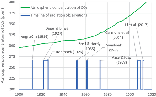
To investigate the two research questions posed in the introduction, we use eight datasets. The first is the earliest dataset by Ångström (1916), and is followed by two datasets used by Brunt (1932) to propose his formula (Robitzsch 1926, Dines and Dines 1927). Then we have three datasets from 1950s, 1960s and 1970s, respectively (Stoll and Hardy 1955, Swinbank 1963, Aase and Idso 1978), two of which were also used by Brutsaert (1991). Finally, we have two datasets of the 21^st century (Carmona et al. 2014, Li et al. 2017), in which the atmospheric CO₂ concentration was much higher than in the other six datasets. The timeline of the observation periods of the eight datasets is shown in Fig. 1, along with the global atmospheric CO₂ concentration.

Figure 1. Timeline of the observation periods of the eight datasets (not to scale) and atmospheric CO₂ concentration according to Meinshausen et al. (2020). The CO₂ concentration data were downloaded from https://gmd.copernicus.org/articles/13/3571/2020/gmd-13-3571-2020-supplement.zip (accessed 25 August 2023); from the Microsoft Excel file provided at that URL, the data from the column “CO₂ ppm World” of the tabs “T2 – History Year 1750 to 2014” were retrieved.

The details of the datasets are given in Table 1. All datasets used are for clear-sky conditions, which is most appropriate for our purpose as they exclude any interference from clouds. In addition to the eight datasets, the measurements by Goss and Brooks (1956), which were the basis of the FAO Penman-Monteith method, were also retrieved, by digitization of their fig. 4, and analysed, but they were not included in Table 1 as the information provided was not enough to make even a rough reconstruction.

Table 1. Details of the eight datasets used in the study and information about their retrieval.

Dataset no.	Observation year [CO2 concentration], References	Notes
1	1912 [300 ppm] Ångström (1916)	This is probably the earliest record of systematic measurements of $L_{\mathrm{n}}$ (38 in total), conducted by Ångström in Bassour, Algeria, during July–September 1912. The results of all measurements are tabulated in his publication. No preprocessing of the data was necessary except conversion to SI units.
2	1922–1926 [305 ppm] Dines and Dines (1927), Brunt (1932, 1934), Swinbank (1963)	This dataset was the basis of the celebrated Brunt formula, Equation (7)(7) ${\epsilon }_{\mathrm{a}}=0.526+0.065\sqrt{e_{\mathrm{a}}/\mathrm{hPa}}$(7) . The publication by Dines and Dines (1927) contained tables with observations of radiation, including longwave, at Benson, Oxfordshire, UK, during 1922–1926. The tables, which according to Raman (1935) contained 12 monthly mean values, were not found. However, it was possible to make a useful reconstruction of the dataset (ranges rather than individual values), based on the facts that: (a) Brunt (1932, 1934) reports a near perfect correlation with respect to Equation (7), with a correlation coefficient of 0.97; (b) Brunt (1932, 1934) gives the range of $\mathit{e}$ as 7–14 hPa; (c) Swinbank’s (1963) fig. 1 shows that $L_{\mathrm{a}}$ ranged between 237 and 326 $\mathrm{W}{\mathrm{m}}^{-2}$.
3	1926 [306 ppm] Robitzsch (1926), Brunt (1932, 1934), Pekeris (1934)	The original publication by Robitzsch (1926), which contained the measurements, was not found, but his measurements (11 grouped means from 1350 observations taken on 30 clear nights at Lindenberg) were reproduced in tabulated form by Brunt (1932, 1934) and Pekeris (1934). The tabulated data were used here after converting $\mathit{e}$ from mmHg to hPa and recovering from the incorrect value of $\mathit{\sigma }$. Note, though, that Raman (1935) criticized the measurements as possibly influenced by systematic errors.
4	1952–1953 [314 ppm] Stoll and Hardy (1955), Satterlund (1979)	The observations by Stoll and Hardy (1955) were made in Alaska and included some measurements for temperatures below 0°C (down to −55°C). Satterlund (1979, fig. 1), followed by Brutsaert (1991, fig. 6.7), provided these data in graphical form, including in the same convention followed here (see section 4), i.e. $R_{\mathrm{a}}$ calculated by the Brutsaert formula (Equation (4)(4) ${\epsilon }_{\mathrm{a}}=1.24{\left(\frac{{\mathit{e}}_{\mathrm{a}}/\mathrm{hPa}}{T_{\mathrm{a}}/\mathrm{K}}\right)}^{1/7}$(4) ) vs. measured. Satterlund’s figure was digitized, and the units were converted to SI, i.e. from langleys per day ($\mathrm{Ly}{\mathrm{d}}^{-1}=\mathrm{cal}\mathrm{c}{\mathrm{m}}^{-2}{\mathrm{d}}^{-1}$) to $\mathrm{W}{\mathrm{m}}^{-2}$.
5	1961–1962 [318 ppm] Swinbank (1963)	Swinbank (1963) conducted and presented in tabulated form measurements in Australia during 1961–1962, namely Aspendale and Kerang (86 and 5 measurements, respectively), as well as in the Indian Ocean (6 measurements in 1962). The tabulated data were ready for use after the necessary conversion to SI and recovering from the incorrect value of $\mathit{\sigma }$.
6	1973–1974 [330 ppm] Aase and Idso (1978)	Aase and Idso (1978) conducted 65 measurements of longwave radiation at Sidney, Montana, USA (39 for temperatures above 0°C, up to 27°C, and 26 for temperatures below 0°C, down to −30°C). They provided the data in tables, from which they were taken here after conversion from $\mathrm{Ly}{\mathrm{d}}^{-1}$ to $\mathrm{W}{\mathrm{m}}^{-2}$. In addition, Satterlund (1979, fig. 1), followed by Brutsaert (1991, fig. 6.7), provided these data in graphical form, which was cross-checked here and found to agree with the original data.
7	2007–2010 [385 ppm] Carmona et al. (2014)	Carmona et al. (2014) collected data from Tandil in the central-southeastern area of the Buenos Aires province, Argentina, in eight measurement campaigns. The measurements, taken over 840 days, included 3443 hourly observations for clear-sky conditions. As shown in their fig. 2, $L_{\mathrm{a}}$ ranged between 200 and 450 $\mathrm{W}{\mathrm{m}}^{-2}$, $T_{\mathrm{a}}$ between 0 and 36°C, and $\mathit{U}$ between 0.1 and 1. The data are provided in graphical form, including in the same convention followed here (see section 4), i.e. $R_{\mathrm{a}}$ calculated by the Brutsaert formula (Equation (4)(4) ${\epsilon }_{\mathrm{a}}=1.24{\left(\frac{{\mathit{e}}_{\mathrm{a}}/\mathrm{hPa}}{T_{\mathrm{a}}/\mathrm{K}}\right)}^{1/7}$(4) ) vs. measured. The related graph (Carmona et al. 2014, fig. 3d) was digitized and the resulting values, which were originally in SI units, were then ready for processing. It is expected that, because of the large size of the dataset, some of the data points were not identified by the automatic digitization software, but the resulting cloud of points looks identical to that of the original graph.
8	2012–2013 [395 ppm] Li et al. (2017)	Li et al. (2017) processed data from seven Surface Radiation Budget Network (SURFRAD) stations over the contiguous USA covering different climatic conditions and an altitude span from 98 m to 1689 m. Their comprehensive dataset includes 17 127 and 14 052 measurements for clear-sky conditions for 2012 and 2013, respectively. Because of the huge number of data points, their plots illustrate only a random subset to improve the readability of the figures. Therefore, recovery of the data by digitization of their figures was impossible. However, it was possible to make a representative reconstruction of the dataset (ranges rather than individual values), based on the facts that: (a) Li et al. provide a near-perfect recalibration of the Brutsaert formula (Equation (4)(4) ${\epsilon }_{\mathrm{a}}=1.24{\left(\frac{{\mathit{e}}_{\mathrm{a}}/\mathrm{hPa}}{T_{\mathrm{a}}/\mathrm{K}}\right)}^{1/7}$(4) ) on their data, with relative bias of −0.6% and root mean square error (RMSE) of 4.5%; the recalibrated parameters are 1.168 and 1/9, replacing 1.24 and 1/7, respectively; (b) their fig. 2 indicates that $L_a$ ranged between 170 and 450 $\mathrm{W}{\mathrm{m}}^{-2}$; (c) their table 1 provides interquartile ranges for $T_{\mathrm{a}}$, $L_{\mathrm{a}}$ and $\mathit{U}$. Details of the reconstruction method are given in Appendix A.

4 Results

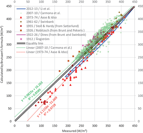
The method we use to deal with the two research questions is simple, intuitive and graphical. Specifically, for each dataset, we plot the calculated values of the downward longwave radiation $L_{\mathrm{a}}$ against the measured values. The plots for all eight datasets are shown in a single graph, Fig. 2, which allows comparison of each dataset with the equality line (calculated $L_{\mathrm{a}}$ equal to measured) as well as intercomparisons of the behaviours of the different datasets.

Figure 2. Plot of downward radiation of the atmosphere L_a calculated by Brutsaert’s formula with its original parameters (Equation (4)(4) ${\epsilon }_{\mathrm{a}}=1.24{\left(\frac{{\mathit{e}}_{\mathrm{a}}/\mathrm{hPa}}{T_{\mathrm{a}}/\mathrm{K}}\right)}^{1/7}$(4) ) vs. measured L_a in all eight datasets. The points correspond to individual measurements, while the lines correspond to reconstructions by envelopes, as described in Table 1 and Appendix A. For the two datasets with the largest number of points (Aase and Idso 1978 and Carmona et al. 2014), the linear regression lines are also shown in the figure, along with their equations.

To find the calculated values we use a single reference model, namely Brutsaert’s formula (Equation (4)(4) ${\epsilon }_{\mathrm{a}}=1.24{\left(\frac{{\mathit{e}}_{\mathrm{a}}/\mathrm{hPa}}{T_{\mathrm{a}}/\mathrm{K}}\right)}^{1/7}$(4) ) with its original parameters, so that we have the same reference for all datasets. The reasons we chose this formula are the following: (a) it has a strong theoretical background; (b) in the study by Carmona et al. (2014), which among other things compared six methods (with their original parameters) against their set of observations (dataset No. 7 in Table 1), it was ranked first in terms of performance; (c) in the study by Guo et al. (2019), which compared five methods against ground measurements collected from 71 globally distributed sites, Brutsaert’s formula was found to perform most uniformly with respect to altitude, having the largest coefficient of determination and lowest bias for high altitudes (> 3000 m, in which temperatures are lower); (d) it was deemed most relevant from a hydrological perspective (Wilfried Brutsaert is a hydrologist).

As seen in Fig. 2, deviations from the equality line are visible and reflect: (a) differences in the local conditions as the datasets are observations from different parts of the world with different climates; (b) differences in the temperature lapse rate and water vapour profile at different times, even for the same location; (c) differences in aerosols in the atmosphere; (d) different measurement errors as the measuring devices have changed over the century-long period; and (e) imperfections of Brutsaert’s formula, which is based on several assumptions about the profiles of atmospheric variables – assumptions that may not always hold.

Actually, these very deviations constitute the conceptual basis of our method. Our aim is to investigate whether they follow a systematic pattern, with respect to the time period of the measurements, and hence the CO₂ concentration, which has been systematically increasing in time. With reference to Fig. 2, if a particular dataset indicates an enhanced greenhouse effect, the measured values would be higher than the calculated ones as the latter refer to the standard reference conditions. Therefore the data points will be aligned on the right of the equality line. In contrast, a weaker greenhouse effect will be seen as an alignment of the points on the left of the equality line. An enhancement of the greenhouse effect, due to increasing CO₂ concentration, through the years would be seen as a gradual displacement of the points from left to right with the progression of time.

However, the alignment of points of the different datasets does not show a gradual displacement from left to right. Rather it shows alternation in both directions. This means that the effect of the direct CO₂ emission at the surface is smaller than the side effects (listed as (a) to (e) above) causing the variability seen in Fig. 2, and thus it is impossible to discern. For the two datasets with the larger number of points, Aase and Idso (1978) for 330 ppm CO₂, and Carmona et al. (2014) for 385 ppm CO₂, the linear regression lines have also been drawn in the figure. These are aligned opposite to the expectation of displacement, i.e. the older set lies on the right of the equality line and the newer on the left.

The measurements by Goss and Brooks (1956), which were the basis of the FAO Penman-Monteith method, were also analysed, assuming several alternatives of $\mathit{U}$ for the individual measurements, as there was no hint about the values of $\mathit{U}$ or $\mathit{T}$ in the paper. These alternatives resulted in large differences among them, yet in all of them the resulting points were aligned very close to the equality line (closer than most of the other datasets).

Generally, Brutsaert’s formula (Equation (4)(4) ${\epsilon }_{\mathrm{a}}=1.24{\left(\frac{{\mathit{e}}_{\mathrm{a}}/\mathrm{hPa}}{T_{\mathrm{a}}/\mathrm{K}}\right)}^{1/7}$(4) ), which is mapped as the equality line in the figure, represents well all datasets, irrespective of time or CO₂ concentration. Additional factors such as those listed above (points (a) to (e)) can influence the greenhouse effect and thus cause differences in $L_{\mathrm{a}}$, which are not captured by Brutsaert’s formula or other ones.

A recent development has given water an additional role in this respect, which needs to be explored. Specifically, according to the standard assumptions, the concentration of H₂O above the troposphere is very small, on the order of 1 ppm (van Wijngaarden and Happer 2020, fig. 1), and hence its contribution to the greenhouse effect is negligible in the upper strata of the atmosphere. However, following the Hunga Tonga-Hunga Ha’apai submarine volcanic eruption (15 January 2022), an enormous H₂O injection was observed, which penetrated even into the mesosphere (Millán et al. 2022). As a result, H₂O concentrations in the upper strata of the atmosphere increased even by two orders of magnitude, up to the order of 100 ppm (Millán et al. 2022, fig. 3), while in the stratosphere the water mass increased by 13% relative to climatological levels (Khaykin et al. 2022). Millán et al. (2022) asserted that the excess stratospheric H₂O will persist for years, and may lead to surface warming due to the radiative forcing from the excess stratospheric H₂O.

5 Conclusions

The various sets of observations of Earth’s atmospheric (longwave) radiation, spanning a period of a century, allow us to draw the following conclusions, which answer the research questions posed in the introduction:

1. The observed increase of the atmospheric CO₂ concentration from 300 to more than 400 ppm has not altered, in a discernible manner, the greenhouse effect, which remains dominated by the quantity of water vapour in the atmosphere.

2. The original formulae used in hydrological practice, in particular those related to the longwave radiation in the framework of evaporation calculations, remain valid and they do not need adaptation due to increased CO₂ concentration.

Apparently, this does not mean that further research is unnecessary, or that we have reached a “settled science” (a popular term, which may be interpreted as a euphemism for unsettled – cf. Koonin 2021). Rather, the results of this study suggest that this further research should move the focus from the influence of carbon dioxide on climate to that of water. The recent incident of the submarine volcanic eruption, which caused an enormous increase in the water concentration in the upper atmosphere, also highlights the necessity of studying the multifaceted role of water in the greenhouse effect.

Data availability

This research uses no new data. The datasets used have been retrieved from the sources described in detail in the text.

Acknowledgements

We are grateful to the Editor Attilio Castellarin and two anonymous reviewers for their positive evaluation of our paper and for their very constructive comments, including their criticisms, which triggered an expansion of the study and the addition of Appendix B, not contained in the original version.

Disclosure statement

No potential conflict of interest was reported by the authors.

Additional information

Funding

This research received no funding but was conducted for scientific curiosity.

Notes

¹ Long-range predictions may contradict Karl Popper’s (1983) falsifiability principle, i.e. “[a] statement (a theory, a conjecture) has the status of belonging to the empirical sciences if and only if it is falsifiable.” In addition, the following quotation by Percy Williams Bridgman (1966) may hold: “A combination of words in the grammatical form of statement is only a ‘pseudo-statement’ when it purports to be about the future.” More specific information about future climate predictions (also known as projections) can be found in Koutsoyiannis et al. (2008, 2011, 2023b) and Koutsoyiannis (2020).

² Examples are the following quotations: (a) “Carbon dioxide is Earth’s most important greenhouse gas” (US National Oceanic and Atmospheric Administration – NOAA, Climate.gov: Science & information for a climate-smart nation, https://www.climate.gov/news-features/understanding-climate/climate-change-atmospheric-carbon-dioxide; (b) “Carbon dioxide is widely reported as the most important anthropogenic greenhouse gas” (US Environmental Protection Agency – EPA, Report on the Environment, https://www.epa.gov/report-environment/greenhouse-gases; notice here the adjective “anthropogenic,” but note that in fact only 4% of the carbon dioxide emissions are anthropogenic, with 96% being natural; Koutsoyiannis et al. 2023b); (c) “For climate change, the most important greenhouse gas is carbon dioxide, which is why you hear so many references to ‘carbon’ when people talk about climate change” (Massachusetts Institute of Technology – MIT, Climate Portal, https://climate.mit.edu/explainers/greenhouse-gases); (d) “Carbon dioxide (CO₂) is the most significant greenhouse gas” (Britannica, https://www.britannica.com/science/greenhouse-gas). (All linked sites were accessed on 15 October 2023).

Appendix A:

Reconstruction of the Li et al. dataset

Here we provide details for the reconstruction of the Li et al. (2017) dataset, for the purpose of comparing it with other datasets in Fig. 2. We stress that this reconstruction is made in terms of envelope curves rather than individual values, which would be impossible. We interpreted the values resulting from the recalibrated parameters of Brutsaert’s formula by Li et al. as measured values and we used the original parameters to find the calculated values of $L_{\mathrm{a}}$. Obviously, this method does not capture the (likely random) error around Li et al.’s recalibrated model (RMSE = 4.5%) and therefore the term “envelope” is not meant in its precise sense, but after removing the error. Certainly, however, the method captures the general tendency of the data.

If $\mathit{M}$ is the “measured” atmospheric radiation, which corresponds to the calibrated parameters of Brutsaert’s formula by Li et al. (2017), and $\mathit{C}$ is the calculated atmospheric radiation, which corresponds to the standard Brutsaert formula (Equation (4)(4) ${\epsilon }_{\mathrm{a}}=1.24{\left(\frac{{\mathit{e}}_{\mathrm{a}}/\mathrm{hPa}}{T_{\mathrm{a}}/\mathrm{K}}\right)}^{1/7}$(4) ), then

(A1) $\mathit{M}=1.168{\left(\frac{{\mathit{e}}_{\mathrm{a}}}{T_{\mathrm{a}}}\right)}^{0.111}\mathit{\sigma }{T}_{\mathrm{a}}^4,\mathit{C}=1.24{\left(\frac{{\mathit{e}}_{\mathrm{a}}}{T_{\mathrm{a}}}\right)}^{0.143}\mathit{\sigma }{T}_{\mathrm{a}}^4$(A1)

where all quantities are expressed in the usual SI units ($\mathit{M}$ and $\mathit{C}$ in $\mathrm{W}{\mathrm{m}}^{-2},$ $T_{\mathrm{a}}$ in K, $e_{\mathrm{a}}$ in hPa). Assuming that the temperature $T_{\mathrm{a}}$ is specified, we eliminate $e_{\mathrm{a}}$ from these two equations, and after algebraic manipulations we find

(A2) $\mathit{C}=1.015M^{1.287}{\left(\sigma T_{\mathrm{a}}^4\right)}^{-0.287}=122\frac{{\mathit{M}}^{1.287}}{T_{\mathrm{a}}^{1.148}}$(A2)

Alternatively, in the case that the relative humidity $\mathit{U}=e_{\mathrm{a}}/\mathit{e}\left(T_{\mathrm{a}}\right)$ is specified, we have

(A3) $\mathit{M}=1.168{\left(\frac{\mathit{Ue}\left({\mathit{T}}_{\mathrm{a}}\right)}{T_{\mathrm{a}}}\right)}^{0.111}\mathit{\sigma }{T}_{\mathrm{a}}^4,\mathit{C}=1.24{\left(\frac{\mathit{Ue}\left({\mathit{T}}_{\mathrm{a}}\right)}{T_{\mathrm{a}}}\right)}^{0.143}\mathit{\sigma }{T}_{\mathrm{a}}^4$(A3)

These two equations again define a relationship between $\mathit{M}$ and $\mathit{C}$ – which, however, is implicit as it involves $T_{\mathrm{a}}$, which is not specified. Nonetheless, the relationship between $\mathit{M}$ and $\mathit{C}$ is well defined and can be evaluated numerically.

Now, for the reconstruction we assumed $L_a$ between 170 to 450 $\mathrm{W}{\mathrm{m}}^{-2}$, and we constructed three envelope curves. For the upper curve shown in Fig. 2 (the one that is almost a straight line) we assumed $\mathit{U}=1$ (the upper physical limit) and used Equation (A3) to determine $\mathit{C}$ from $\mathit{M}$. The lower curve is in fact a concatenation of two parts. The lower part corresponds to $\mathit{U}=0.1$ (a reasonable minimum of relative humidity, smaller than the lower quantile in the most arid station, which is 0.134) and was again calculated using Equation (A3). The high part corresponds to $T_{\mathrm{a}}=30$ °C (a reasonable maximum of temperature, greater than the upper quantile in the most arid station, which is 27.1°C) and was calculated using Equation (A2).

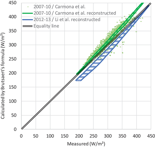
To cross-check the performance of the method of reconstruction by envelopes, we also applied it to the dataset of Carmona et al. (2014), for which the entire data series is available. In addition, Carmona et al. also recalibrated Brutsaert’s formula. The fitted parameters in both studies are shown in Table A1, along with the original parameters. The resulting envelopes for $\mathit{U}=1$, $\mathit{U}=0.1$ and $T_{\mathrm{a}}=36$ °C (see Table 1, dataset No. 7) are shown in Fig. A1, along with the individual points and, for comparison, the envelopes for the Li et al. (2017) dataset.

The envelopes for the Carmona et al. dataset are well aligned with respect to the spread of the individual points (also plotted in the figure), but, as expected, they do not capture the entire scatter of the data. Nonetheless, they capture the tendency of the data to lie on the left of the equality line, while the reconstruction of the Li et al. data lies on the right of the equality line. Interestingly, in both studies, both fitted parameters are smaller than in the original formula (Table A1) and one would intuitively expect a similar behaviour for the two datasets. However, the smaller value of $\mathit{b}$ given by Li et al. results in the opposite alignment of the envelopes with respect to the equality line (Fig. A1).

Table A1. Parameters $a^{\prime }$ and $b^{\prime }$ of the generalized Brutsaert formula, ${\epsilon }_{\mathrm{a}}=a^{\prime }{\left({\mathit{e}}_{\mathrm{a}}/T_{\mathrm{a}}\right)}^{\mathit{b}{ }^{\mathrm{\prime }}}$, as recalibrated by Carmona et al. (2014) and Li et al. (2017), and the resulting relative RMSE of the fitting as reported in these publications.

	Original: Brutsaert (1975)	Carmona et al. (2014)	Li et al. (2017)
$a^{\prime }$	1.24	1.11	1.168
$b^{\prime }$	1/7 = 0.143	0.123	1/9 = 0.111
Relative RMSE		4%	4.5%

Figure A1. Cross-check of the reconstruction by envelopes based on the Carmona et al. (2014) dataset, for which both the original points and the envelopes are shown. The reconstruction of Li et al. (2017) is also shown for comparison. The graph is similar to that of Fig. 2, showing the downward radiation of the atmosphere L_a calculated by the Brutsaert formula with its original parameters (Equation (4)(4) ${\epsilon }_{\mathrm{a}}=1.24{\left(\frac{{\mathit{e}}_{\mathrm{a}}/\mathrm{hPa}}{T_{\mathrm{a}}/\mathrm{K}}\right)}^{1/7}$(4) ), vs. measured or reconstructed L_a, but only for the two indicated sets. The points correspond to individual measurements, while the lines correspond to reconstructions by envelopes.

Appendix B:

Radiation data in the top of the atmosphere

Harries et al. (2001) analysed the spectra of the outgoing longwave radiation of the Earth as measured by orbiting spacecraft in 1970 vs. 1997 and found differences that point to long-term changes in atmospheric CO₂ and other gases related to the greenhouse effect. Their study considered the profiles of atmospheric temperature and water vapour, but did not give any hint of the relative contribution (and importance) of water vapour in comparison to these gases. In a macroscopic approach, like the one followed in this paper, it is the total longwave radiation flux rather than the changes in the spectrum for particular frequencies that counts most.

In the 21st century, radiation fluxes at the top of the atmosphere (TOA) have been estimated from satellite instruments. Specifically, this was done in the ongoing project Clouds and the Earth’s Radiant Energy System (CERES), a part of NASA’s Earth Observing System, designed to measure both solar-reflected and Earth-emitted radiation from the TOA (in CERES defined at an altitude of 20 km) to the surface. The data are available from https://ceres-tool.larc.nasa.gov/ord-tool/jsp/SSF1degEd41Selection.jsp and were retrieved here as global averages for the monthly time scale and for their entire time span, which is from March 2000 to the present for the Terra platform and from July 2002 to the present for the Aqua platform.

The CERES TOA time series of longwave radiation fluxes for clear sky and all sky conditions are shown in Fig. B1. The graphs also show the linear trends in the two cases, which were estimated for full years only (i.e. 23 years for the Terra platform and 20 years for the Aqua platform, leaving out a number of values exceeding a multiple of 12). The linear trends are very small. What is more interesting is that, while they are slightly negative for clear sky, they become slightly positive for all sky. This does not suggest that they are linked to CO₂ changes. Rather, a link to atmospheric water is more likely, as it can be conjectured that they reflect changes in the temperature and water vapour profiles in the atmosphere and hence in the formation and vertical profiles of clouds.

To better assess a possible connection with water and, in particular, its form in clouds (which are opaque to shortwave radiation), we also examine the time series of shortwave radiation, whose temporal evolution is shown in Fig. B2. The latter figure indicates a falling trend, which is clearer and a multiple of that of clear sky longwave radiation (Fig. B1). Note that the decreasing trend in total outgoing TOA radiation flux is consistent with increased atmospheric temperature (decreased total outgoing radiation flux means that more energy is stored on Earth). From the numerical values of the trends in the two figures we find that the total decrease of outgoing radiation in the 23 years of data availability is (0.649 – 0.137) × 23/10 = 1.18 W/m². This is greater than the average imbalance (net absorbed energy) of the Earth, which, if calculated from the ocean heat content data, is about 0.4 W/m² (Koutsoyiannis 2021). This decrease of outgoing radiation can hardly be attributed to increased CO₂ concentration. Rather, it can be related to water vapour and cloud profiles (and aerosols), given that other greenhouse gases such as CO₂ and CH₄ are well mixed.

It would not be surprising if someone attributed the trends in Figs B1 and B2 to some factor related to the commonly assumed hydrological intensification caused by the rising CO₂ concentration. However, as shown by Koutsoyiannis (2020), the IPCC assumptions on the intensification of the hydrological cycle due to CO₂ increase do not stand. Additional support on this is provided by Fig. B3, where macroscopically no increasing trend (actually no trend at all) is seen in the atmospheric water content.

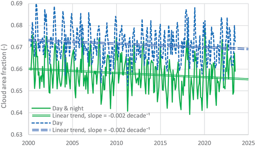
In contrast, as shown in Fig. B4, decreasing trends appear in the total cloud area fraction. This is consistent with the above conjecture that changes in the shortwave radiation are related to changes in clouds; those in the longwave radiation are more difficult to explain and one would need to study the profiles and geographical distribution of temperature, water vapour and clouds.

The above information cannot give conclusive results as the period of measurement is short and the processes too complex to allow for a simple interpretation. Yet all indications suggest that at the macroscopic level (global fluxes) the changes observed are related to water, while nothing related to CO₂ is discerned. This suggests a minor role of CO₂, as substantiated by van Wijngaarden and Happer (2020) and de Lange et al. (2022), and also expressed by Smirnov and Zhilyaev (2021, p. 197) in their statement “water molecules in the atmosphere may be responsible for the observed heating of the Earth,” which is in “contradiction with the results of climatological models in the analysis of the Earth’s greenhouse effect.” The difference in the conclusions of Harries et al. (2001) on the one hand and the three studies mentioned just above on the other hand must lie in the fact the latter investigated the entire range of longwave frequencies from 0 to 2500 – 2600 cm⁻¹, while the former examined frequencies in the range of 700 to 1400 cm⁻¹. Interestingly, the frequencies left out by Harries et al. (2001) (i.e. < 700 cm⁻¹ and > 1400 cm⁻¹) are precisely those fully dominated by water molecules.

Figure B1. TOA time series of longwave radiation fluxes, as provided by NASA’s CERES, along with linear trend, for (a) all sky and (b) clear sky.

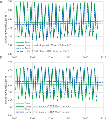
Figure B2. TOA time series of shortwave radiation flux, as provided by NASA’s CERES, along with linear trend, for all sky.

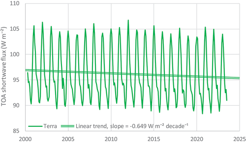
Figure B3. Atmospheric water content (precipitable water), as provided by NASA’s CERES, along with linear trend (which in this case does not exist).

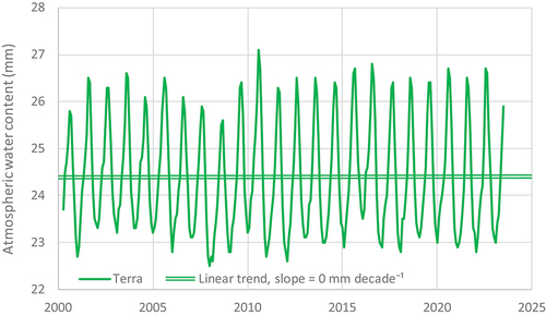
Figure B4. Total cloud area fraction, as provided by NASA’s CERES, along with linear trends.

References

- Aase, J.K. and Idso, S.B., 1978. A comparison of two formula types for calculating long‐wave radiation from the atmosphere. Water Resources Research, 14 (4), 623–625. doi:10.1029/WR014i004p00623
- Allan, R.P., 2009. Examination of relationships between clear-sky longwave radiation and aspects of the atmospheric hydrological cycle in climate models, reanalyses, and observations. Journal of Climate, 22 (11), 3127–3145. doi:10.1175/2008JCLI2616.1
- Allen, R.G., et al., 1998. Crop evapotranspiration – guidelines for computing crop water requirements. FAO Irrigation and Drainage Paper 56, Rome: Food and Agriculture Organization of the United Nations. Available from: https://www.fao.org/3/X0490E/x0490e00.htm [ Accessed 25 August 2023].
- Ångström, A., 1916. A study of the radiation of the atmosphere based upon observations of the nocturnal radiation during expeditions to Algeria and to California. Smithsonian Miscellaneous Collections, 65 (3), 159. Available from; https://archive.org/details/smithsonianmisce651916smit/ [ Accessed 25 August 2023].
- Arrhenius, S., 1896. XXXI. On the influence of carbonic acid in the air upon the temperature of the ground. The London, Edinburgh, and Dublin Philosophical Magazine and Journal of Science, 41 (251), 237–276. doi:10.1080/14786449608620846
- Asklöf, S., 1920. Über Den Zusammenhang Zwischen Der Nächtlichen Wärmeaus-Strahlung, Der Bewölkung und Der Wolkenart. Geografiska Annaler, 2 (3), 253–259. doi:10.1080/20014422.1920.11880773
- Batchelor, C.H., 1984. The accuracy of evapotranspiration estimated with the FAO modified Penman equation. Irrigation Science, 5 (4), 223–233. doi:10.1007/BF00258176
- Boutaric, M.A., 1928. Le rayonnement nocturne. La Météorologie, 4, 289–299. Available from: https://gallica.bnf.fr/ark:/12148/bpt6k96361506 [ Accessed 25 August 2023].
- Bridgman, P.W., 1966. The way things are. Cambridge, Mass., USA: Harvard University Press.
- Brooks, F.A., 1941. Observations of atmospheric radiation. Massachusetts Institute of Technology Papers in Physical Oceanography and Meteorology, 8 (2), 1–23. Available from: https://core.ac.uk/download/pdf/4165621.pdf [ Accessed 25 August 2023].
- Brooks, F.A., 1952. Atmospheric radiation and its reflection from the ground. Journal of the Atmospheric Sciences, 9 (1), 41–52.
- Brunt, D., 1932. Notes on radiation in the atmosphere. I. Quarterly Journal of the Royal Meteorological Society, 58 (247), 389–420. doi:10.1002/qj.49705824704
- Brunt, D., 1934. Physical and Dynamical Meteorology. Cambridge, UK: Cambridge University Press, 411. Available from: https://archive.org/details/in.ernet.dli.2015.215092 [ Accessed 25 August 2023].
- Brutsaert, W., 1975. On a derivable formula for long‐wave radiation from clear skies. Water Resources Research, 11 (5), 742–744. doi:10.1029/WR011i005p00742
- Brutsaert, W., 1991. Evaporation into the atmosphere: theory, history and applications. Dordrecht, Netherlands: Springer Science & Business Media, 299.
- Canadell, J.G., et al., 2021. Global carbon and other biogeochemical cycles and feedbacks. In: V. Masson-Delmotte, et al., eds. Climate change 2021: the physical science basis. Contribution of working group I to the sixth assessment report of the intergovernmental panel on climate change. Cambridge, United Kingdom and New York, NY, USA: Cambridge University Press, 673–816. doi:10.1017/9781009157896.007
- Carmona, F., Rivas, R., and Caselles, V., 2014. Estimation of daytime downward longwave radiation under clear and cloudy skies conditions over a sub-humid region. Theoretical and Applied Climatology, 115 (1–2), 281–295. doi:10.1007/s00704-013-0891-3
- de Lange, C.A., et al., 2022. Nitrous oxide and climate. arXiv, arXiv:2211.15780 Available from: https://arxiv.org/abs/2211.15780 [ Accessed 25 August 2023].
- Dimitriadis, P., et al., 2021. A global-scale investigation of stochastic similarities in marginal distribution and dependence structure of key hydrological-cycle processes. Hydrology, 8 (2), 59. doi:10.3390/hydrology8020059
- Dines, W.H., 1920. Atmospheric and terrestrial radiation. Quarterly Journal of the Royal Meteorological Society, 46 (194), 163–174. doi:10.1002/qj.49704619405
- Dines, W.H. and Dines, L.H.G., 1927. Monthly mean values of radiation from various parts of the sky at Benson, Oxfordshire. Memoirs of the Royal Meteorological Society, 2, 11.
- Doorenbos, J. and Pruitt, W.O., 1977. Guidelines for predicting crop water requirements. FAO Irrigation and Drainage Paper 24, p. 145. Rome: Food and Agriculture Organization of the United Nations. Available from: https://dokumen.tips/download/link/fao-irrigation-and-drainage-paper-24.html [ Accessed 25 August 2023].
- Elsasser, W.M., 1942. Heat transfer by infrared radiation in the atmosphere. Milton, Massachusetts, USA: Harvard University Blue Hill Meteorological Observatory. Available from: https://archive.org/details/ElsasserFull1942 [ Accessed 25 August 2023].
- Essex, C. and Tsonis, A.A., 2018. Model falsifiability and climate slow modes. Physica A Statistical Mechanics & Its Applications, 502, 554–562. doi:10.1016/j.physa.2018.02.090
- Goody, R.M., 1964. Atmospheric Radiation. Oxford, UK/New York: Oxford University Press USA, 436.
- Goss, J.R. and Brooks, F.A., 1956. Constants for empirical expressions for downcoming atmospheric radiation under cloudless sky. Journal of Atmospheric Sciences, 13 (5), 482–487.
- Guo, Y., Cheng, J., and Liang, S., 2019. Comprehensive assessment of parameterization methods for estimating clear-sky surface downward longwave radiation. Theoretical and Applied Climatology, 135 (3–4), 1045–1058. doi:10.1007/s00704-018-2423-7
- Harries, J., et al., 2001. Increases in greenhouse forcing inferred from the outgoing longwave radiation spectra of the Earth in 1970 and 1997. Nature, 410 (6826), 355–357. doi:10.1038/35066553
- Hurst, H.E., 1951. Long term storage capacities of reservoirs. Trans. Am. Soc. Civil Eng, 116, 776808.
- Khaykin, S., et al., 2022. Global perturbation of stratospheric water and aerosol burden by Hunga eruption. Communications Earth & Environment, 3 (1), 316. doi:10.1038/s43247-022-00652-x
- Klemeš, V., 1986. Operational testing of hydrological simulation models. Hydrological Sciences Journal, 31 (1), 13–24. doi:10.1080/02626668609491024
- Klemeš, V., 2007. 20 years later: what has changed – and what hasn’t. In XXIV general assembly of the International Union of Geodesy and Geophysics, Perugia: International Union of Geodesy and Geophysics, International Association of Hydrological Sciences. Available from: http://itia.ntua.gr/831/ [ Accessed 15 October 2023].
- Koonin, S.E., 2021. Unsettled: what climate science tells us, what it doesn’t, and why it matters. Dallas, TX, USA: BenBella Books.
- Koutsoyiannis, D., 2012. Clausius-Clapeyron equation and saturation vapour pressure: simple theory reconciled with practice. European Journal of Physics, 33 (2), 295–305. doi:10.1088/0143-0807/33/2/295
- Koutsoyiannis, D., 2013. Hydrology and change. Hydrological Sciences Journal, 58 (6), 1177–1197. doi:10.1080/02626667.2013.804626
- Koutsoyiannis, D., 2014a. Entropy: from thermodynamics to hydrology. Entropy, 16 (3), 1287–1314. doi:10.3390/e16031287
- Koutsoyiannis, D., 2014b. Reconciling hydrology with engineering. Hydrology Research, 45 (1), 2–22. doi:10.2166/nh.2013.092
- Koutsoyiannis, D., 2019. Time’s arrow in stochastic characterization and simulation of atmospheric and hydrological processes. Hydrological Sciences Journal, 64 (9), 1013–1037. doi:10.1080/02626667.2019.1600700
- Koutsoyiannis, D., 2020. Revisiting the global hydrological cycle: is it intensifying? Hydrology and Earth System Sciences, 24 (8), 3899–3932. doi:10.5194/hess-24-3899-2020
- Koutsoyiannis, D., 2021. Rethinking climate, climate change, and their relationship with water. Water, 13 (6), 849. doi:10.3390/w13060849
- Koutsoyiannis, D., 2023. Stochastics of hydroclimatic extremes – a cool look at risk. 3rd ed. Athens: Kallipos Open Academic Editions, 391. Available from: https://www.itia.ntua.gr/2000/ [ Accessed 25 August 2023].
- Koutsoyiannis, D., et al., 2011. Scientific dialogue on climate: is it giving black eyes or opening closed eyes? Reply to “A black eye for the hydrological sciences journal” by D. Huard. Hydrological Sciences Journal, 56 (7), 1334–1339. doi:10.1080/02626667.2011.610759
- Koutsoyiannis, D., et al., 2008. On the credibility of climate predictions. Hydrological Sciences Journal, 53 (4), 671–684. doi:10.1623/hysj.53.4.671
- Koutsoyiannis, D., et al., 2023a. In search of climate crisis in Greece using hydrological data: 404 not found. Water, 15 (9), 1711. doi:10.3390/w15091711
- Koutsoyiannis, D. and Kundzewicz, Z.W., 2020. Atmospheric temperature and CO₂: hen-or-egg causality? Sci, 2 (3), 72. doi:10.3390/sci2040077
- Koutsoyiannis, D. and Mamassis, N., 2021. From mythology to science: the development of scientific hydrological concepts in the Greek antiquity and its relevance to modern hydrology. Hydrology and Earth System Sciences, 25 (5), 2419–2444. doi:10.5194/hess-25-2419-2021
- Koutsoyiannis, D. and Montanari, A., 2022a. Bluecat: a local uncertainty estimator for deterministic simulations and predictions. Water Resources Research, 58 (1), e2021WR031215. doi:10.1029/2021WR031215
- Koutsoyiannis, D. and Montanari, A., 2022b. Climate extrapolations in hydrology: the expanded Bluecat methodology. Hydrology, 9 (5), 86. doi:10.3390/hydrology9050086
- Koutsoyiannis, D., et al., 2022a. Revisiting causality using stochastics: 1. Theory. Proceedings of the Royal Society A, 478 (2261), 20210836. doi:10.1098/rspa.2021.0836
- Koutsoyiannis, D., et al., 2022b. Revisiting causality using stochastics: 2. Applications. Proceedings of the Royal Society A, 478 (2261), 20210836. doi:10.1098/rspa.2021.0836
- Koutsoyiannis, D., et al., 2023b. On hens, eggs, temperatures and CO2: causal links in earth’s atmosphere. Sci, 5 (3), 35. doi:10.3390/sci5030035
- Li, M., Jiang, Y., and Coimbra, C.F., 2017. On the determination of atmospheric longwave irradiance under all-sky conditions. Solar Energy, 144, 40–48. doi:10.1016/j.solener.2017.01.006
- Manabe, S., Smagorinsky, J., and Strickler, R.F., 1965. Simulated climatology of a general circulation model with a hydrologic cycle. Monthly Weather Review, 93 (12), 769–798. doi:10.1175/1520-0493(1965)093<0769:SCOAGC>2.3.CO;2
- Manabe, S. and Wetherald, R.T., 1967. Thermal equilibrium of the atmosphere with a given distribution of relative humidity. Journal of the Atmospheric Sciences, 24 (3), 241–259. doi:10.1175/1520-0469(1967)024%3C0241:TEOTAW%3E2.0.CO;2
- Meinshausen, M., et al., 2020. The shared socio-economic pathway (SSP) greenhouse gas concentrations and their extensions to 2500. Geoscientific Model Development, 13 (8), 3571–3605. doi:10.5194/gmd-13-3571-2020
- Milanković, M., 1935. Nebeska Mehanika. Beograd, Serbia: Udruženje Milutin Milanković.
- Milanković, M., 1941. Kanon der Erdbestrahlung und seine Anwendung auf das Eiszeitenproblem. Beograd: Koniglich Serbische Akademice.
- Milanković, M., 1998. Canon of Insolation and the Ice-Age Problem. Belgrade: Agency for Textbooks.
- Millán, L., et al., 2022. The Hunga Tonga-Hunga Ha’apai hydration of the stratosphere. Geophysical Research Letters, 49 (13), e2022GL099381. doi:10.1029/2022GL099381
- Monteith, J.L., 1965. Evaporation and environment. Symposia of the Society for Experimental Biology, 19, 205–234.
- Monteith, J.L. and Szeicz, G., 1962. Radiative temperature in the heat balance of natural surfaces. Quarterly Journal of the Royal Meteorological Society, 88 (378), 496–507. doi:10.1002/qj.49708837811
- O’Connell, P.E., O’Donnell, G., and Koutsoyiannis, D., 2023. On the spatial scale dependence of long-term persistence in global annual precipitation data and the Hurst Phenomenon. Water Resources Research, 59 (4). doi:10.1029/2022WR033133
- Pekeris, C.L., 1934. Note on Brunt’s formula for nocturnal radiation of the atmosphere. Astrophysical Journal, 79, 441–444. doi:10.1086/143552
- Penman, H.L., 1948. Natural evaporation from open water, bare soil and grass. Proceedings of the Royal Society of London. Series A. Mathematical and Physical Sciences, 193 (1032), 120–145.
- Philipona, R., et al., 2004. Radiative forcing - measured at Earth’s surface - corroborate the increasing greenhouse effect. Geophysical Research Letters, 31 (3), L03202. doi:10.1029/2003GL018765
- Popper, K., 1983. Realism and the AIM of science. The postscript to the logic of scientific discovery W.W. Bartley III, ed. Totowa, New Jersey, USA: Rowman & Littlefield.
- Prata, A.J., 1996. A new long‐wave formula for estimating downward clear‐sky radiation at the surface. Quarterly Journal of the Royal Meteorological Society, 122 (533), 1127–1151.
- Raman, P.K., 1935. Heat radiation from the clear atmosphere at night. Proceedings of the Indian Academy of Sciences – Section A, 1 (11), 815–821. doi:10.1007/BF03035637
- Ramanathan, K.R. and Desai, B.N., 1932. Nocturnal atmospheric radiation at Poona, a discussion of measurements made during the period January 1930 to February 1931. Gerlands Beiträge zur Geophysik, 35 (1), 68–81. Available from: https://archive.org/details/selectedpapers02unse/ [ Accessed 25 August 2023].
- Ramanathan, V., 1981. The role of ocean-atmosphere interactions in the CO2 climate problem. Journal of the Atmospheric Sciences, 38 (5), 918–930. doi:10.1175/1520-0469(1981)038<0918:TROOAI>2.0.CO;2
- Robinson, G.D., 1947. Notes on the measurement and estimation of atmospheric radiation. Quarterly Journal of the Royal Meteorological Society, 73 (315–316), 127–150. doi:10.1002/qj.49707331510
- Robitzsch, M., 1926. Strahlungsstudien. In: H, Hergesell, ed. die Arbeiten des Preußischen Aeronautischen Observatoriums bei Lindenberg. Braunschweig: Verlag Friedrich Vieweg & Sohn, XV, 194–213.
- Roe, G., 2006. In defense of Milankovitch. Geophysical Research Letters, 33 (24). doi:10.1029/2006GL027817
- Satterlund, D.R., 1979. An improved equation for estimating long‐wave radiation from the atmosphere. Water Resources Research, 15 (6), 1649–1650. doi:10.1029/WR015i006p01649
- Schmidt, G.A., et al., 2010. Attribution of the present-day total greenhouse effect. Journal of Geophysical Research, 115, D20106. doi:10.1029/2010JD014287
- Smirnov, B.M. and Zhilyaev, D.A., 2021. Greenhouse effect in the standard atmosphere. Foundations, 1 (2), 184–199. doi:10.3390/foundations1020014
- Stoll, A.M. and Hardy, J.D., 1955. Thermal radiation measurements in summer and winter Alaskan climates. Eos, Transactions American Geophysical Union, 36 (2), 213–226.
- Swinbank, W.C., 1963. Long‐wave radiation from clear skies. Quarterly Journal of the Royal Meteorological Society, 89 (381), 339–348. doi:10.1002/qj.49708938105
- Tchiguirinskaia, I., Demuth, S., and Hubert, P., 2008. Report of 9th Kovacs Colloquium: river Basins – from hydrological science to water management, 6–7 June, Paris: UNESCO.
- Tyndall, J., 1865. On radiation: Bede lecture. Cambridge University Press Available from: https://archive.org/details/onradiationbede00tyndgoog/ [ Accessed 25 August 2023].
- UNESCO (United Nations Educational, Scientific and Cultural Organization), 1964. Final report, international hydrological decade, intergovernmental meeting of experts. UNESCO House, Paris: UNESCO/NS/188. Available from: http://unesdoc.unesco.org/images/0001/000170/017099eb.pdf [ Accessed 25 August 2023].
- van Wijngaarden, W.A. and Happer, W., 2020. Dependence of Earth’s thermal radiation on five most abundant greenhouse gases. arXiv, arXiv:2006.03098. Available from: https://arxiv.org/abs/2006.03098 [ Accessed 25 August 2023].
- Wong, R.Y., et al., 2023. Critical sky temperatures for passive radiative cooling. Renewable Energy, 211, 214–226. doi:10.1016/j.renene.2023.04.142
- Yevjevich, V., 1968. Misconceptions in hydrology and their consequences. Water Resources Research, 4 (2), 225–232. doi:10.1029/WR004i002p00225