A stochastic framework for rainfall intensity–time scale–return period relationships. Part ΙΙ: point modelling and regionalization over Greece

ABSTRACT

In this work, we formulate a regionalization framework for rainfall intensity–time scale–return period relationships which is applied over the Greek territory. The methodology for single-site estimation is based on a stochastic framework for multi-scale modelling of rainfall intensity which is outlined in the companion paper. Five parameters are first fitted independently for each site and the resulting parameter variability is assessed. Following a systematic investigation of uncertainty and variability patterns, two parameters, i.e. the tail-index and a time scale parameter, are identified as constant in space and estimated using data pooling techniques. The other three parameters are regionalized over Greece by means of spatial interpolation and smoothing techniques that are assessed through cross-validation in a multi-model framework. The regionalization scheme is implemented in a sequential order that allows exploiting rainfall information both from rainfall stations with sub-daily resolution and from the more reliable network of daily raingauges.

KEYWORDS:

• intensity–duration–frequency curves
• rainfall regionalization
• extreme rainfall
• spatial interpolation
• spatial smoothing
• design rainfall
• geostatistical modelling

Editor A. Castellarin; Associate Editor E. Volpi

1 Introduction

One of the most essential requirements for designing and operating water-related infrastructure, such as dams, bridges, water conveyance structures and urban drainage systems, is the ability to obtain reliable rainfall estimates for different time scales and return periods. This information is usually accessible to engineers in the form of mathematical relationships linking the rainfall intensity (or depth) to the reference time scale and the return period, often misnamed as “duration” and “frequency,” respectively. In this work, we use the term “ombrian relationships” (or curves), as in the companion paper by Koutsoyiannis et al. (2024). The identification of these relationships is based on some form of probabilistic analysis of rainfall, typically performed using extreme value distributions, coupled with a model preserving the important scaling properties of rainfall to retain consistency of the model estimates across the different time scales. There are numerous works in the hydrological literature dealing with the construction of such curves (Svensson and Jones 2010, Lanciotti et al. 2022), from early empirical approaches (Sherman 1931, Bernard 1932) to generalized parametric ones, such as the probabilistic approach proposed by Koutsoyiannis et al. (1998) and the approach based on the rainfall simple- or multi-scaling assumption (Burlando and Rosso 1996), as well as other regression-type (“data-driven”) approaches (Overeem et al. 2008, Haruna et al. 2023). A discussion of existing theoretical concepts for point modelling is provided in the companion paper by Koutsoyiannis et al. (2024).

Aside from the derivation of reliable point estimates, a critical requirement for design rainfall is the ability to generalize this information over large scales, also covering the ungauged regions, a process known as “regionalization.” Several methods have been proposed in the literature for regionalization of design rainfall with degrees of complexity varying usually in relation to the spatial scale of interest. For instance, small regions are often treated as homogeneous and common relationships are identified through data pooling approaches (e.g. Hailegeorgis et al. 2013). As the spatial scale and the degree of spatial variability increases for larger regions, it is a common hydrological practice to identify clusters or sub-regions based on measures of hydrological similarity, and to subsequently apply different regional distributions (see e.g. Aron et al. 1987, Trefry et al. 2005, Burn 2014, Forestieri et al. 2018, Iliopoulou and Koutsoyiannis 2022; and national-scale applications described by Svensson and Jones 2010); a type of spatial approach which is often combined with the so-called “index-method” and the L-moments regional framework (Hosking and Wallis 1997). In this respect, various cluster analysis techniques of different algorithmic complexity have been proposed regarding the possibility to consider some parameter(s) of extreme value distributions as invariant or not in the study area (e.g. Lin and Chen 2006, Rao and Srinivas 2008, Cassalho et al. 2019, De Luca and Napolitano 2023). For larger regions and more complicated rainfall regimes, explicit spatial modelling may be employed for one or more of the involved parameters (e.g. Faulkner and Prudhomme 1998, Perica et al. 2009, Deidda et al. 2021, Iliopoulou et al. 2022, Shehu et al. 2023). The latter approach exploits the advances in geographical information systems and regionalization techniques and allows producing estimates of the required parameters at any point over a given grid. In this way, several limitations of traditional approaches are resolved, including the difficulty of identifying homogeneous regions and the occurrence of inconsistencies at the sub-regions’ borders.

Typically, the employed spatial modelling methods include regression analysis (e.g. Faulkner and Prudhomme 1998, Madsen et al. 2017, Ulrich et al. 2020), the inverse distance weighting (IDW) method (Ahrens 2006, Perica et al. 2009, Szolgay et al. 2009, Mascaro 2020, Barbosa et al. 2022), the kriging method and variations thereof (Watkins et al. 2005, Szolgay et al. 2009, Ceresetti et al. 2012, Blanchet et al. 2016, Forestieri et al. 2018, Libertino et al. 2018, Shehu et al. 2023), bilinear surface smoothing methods (Malamos and Koutsoyiannis 2016b, Iliopoulou et al. 2022), smoothing splines (Hutchinson 1995), neural networks (Ceresetti et al. 2012), Bayesian hierarchical models (Jalbert et al. 2022) and nearest neighbours (e.g. Szolgay et al. 2009), among others (see also Claps et al. 2022 for an extended review).

Despite the existence of many interpolation and geostatistical methods, there are various open methodological questions regarding the implementation of the regionalization scheme. For instance, the most straightforward and widely used procedure is the exact interpolation of independently estimated local parameters (e.g. Szolgay et al. 2009, Blanchet et al. 2016, Barbosa et al. 2022, Mascaro 2020). Despite being simple, this approach implemented through an uncontrolled interpolation might propagate measurement errors in the final product and give rise to unrealistic spatial patterns and abrupt changes (Uboldi et al. 2014, Jalbert et al. 2022). Independent estimation also cannot benefit from the opportunity to increase the reliability of uncertain parameters exploiting information from more records, an issue that is particularly relevant for the highly uncertain shape parameter (tail-index) of the extreme value distribution. On the other hand, for the model to reflect the extreme rainfall climatology and retain the physically-based rainfall structure in space, it is necessary to identify the robust local (“at-site”) properties which should be regionalized. Therefore, the preliminary assessment of parameter uncertainty and spatial patterns as well as prior knowledge of the region’s climatology are prerequisites for the regionalization.

Data availability in the region of interest also determines the implementation of the regionalization scheme. As pointed out by Shehu et al. (2023), the requirements for reliable regionalization, i.e. good data density, fine temporal resolution, and long record length, are seldom satisfied together in any given dataset. The same holds true for the rainfall network in Greece, in which the uncertainty due to limited availability of sub-daily data is exacerbated by the complex topography of the mainland and the numerous distanced islands. To compensate for the short length of sub-daily records and their limited spatial coverage in Greece, Koutsoyiannis et al. (1998) proposed to estimate the distribution parameters employing rainfall maxima from the longer daily raingauges. To augment the useful rainfall information, other works suggest the use of disaggregation/rainfall scaling properties to obtain sub-daily estimates from existing daily series (Bara et al. 2009, Courty et al. 2019, Shehu et al. 2023), utilization of covariates available at a denser spatial network (Madsen et al. 2017), typically elevation (Goovaerts 2000), pooling approaches (e.g. Burn 2014, Iliopoulou and Koutsoyiannis 2022, Iliopoulou et al. 2022), spatial resampling techniques (Uboldi et al. 2014), spatial interpolation of the actual rainfall series (Libertino et al. 2018), while recently the use of radar rainfall, reanalysis and satellite data has been proposed as a means to improve the spatial representation of the rainfall regime (e.g. Ombadi et al. 2018, Courty et al. 2019, Lanciotti et al. 2022). Therefore, regardless of the specifications of each modelling framework, common choices to be made are the parameters to be regionalized as well as the type of data and the order of their utilization in the regionalization scheme.

In this paper, we revisit the existing design rainfall curves for Greece, which are estimated on a point basis, and develop for the first time a regional model valid over the entire Greek territory. By revisiting the existing relationships, we intend to benefit from newer data with better temporal and spatial coverage over Greece and explore advanced methodological frameworks for both point-modelling and regionalization. Specifically, the point modelling methodology has been revisited by Koutsoyiannis (2023) under a stochastic framework, providing better physical meaning for the parameters, theoretical consistency, and links to all-scale stochastic modelling (Koutsoyiannis and Iliopoulou 2022). The framework can also be coupled with a new approach for reliable high-order quantile estimation (K-moments, Koutsoyiannis 2019). The theoretical background for the point modelling is presented in detail in the companion paper by Koutsoyiannis et al. (2024). The specific focus of this work is the formulation of the regionalization approach informed by the stochastic behaviour of extreme rainfall, practical data limitations and uncertainty consideration, as well as empirical insights from the point investigation of the parameters. The latter forms the basis of the regional investigation. This is the culmination of a national-scale effort to produce a gridded product for design rainfall parameters all over Greece for the first time (Koutsoyiannis et al. 2023a).

The study is structured as follows. Rainfall data sources and their analysis are described in Section 2. The employed methods are presented in Section 3; the stochastic methodology for the construction of rainfall intensity–time scale and return period relationships is briefly outlined in Section 3.1, while the regionalization models and their implementation are presented in Section 3.2; at-site performance metrics are presented in Section 3.3. Results are presented in Section 4 together with the final product, the performance assessment, and the design rainfall maps. Discussion is provided in Section 5 and conclusions are outlined in Section 6. Results from the point investigation as well as complementary findings from the regionalization are presented in Appendices A and B, respectively.

2 Data

2.1 Study area

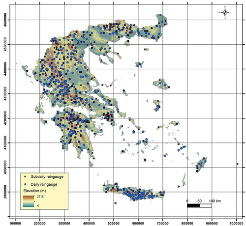
The study area is the Greek territory, comprising a complex topography with an area of 131 957 km² including thousands of islands (Fig. 1). Greek climate is generally characterized as Mediterranean, yet it shows marked spatial diversity in terms of its rainfall regime, with average daily precipitation ranging geographically within an order of magnitude, from 0.6 mm/d (219 mm/year) to 7.3 mm/d (2666 mm/year) (Koutsoyiannis et al. 2023b). The wettest part is northwestern Greece, while the driest parts include Athens, some of the Aegean islands, and parts of central Macedonia and Thessaly.

Figure 1. Elevation map of Greece along with the locations of the daily and sub-daily resolution rainfall stations used in the analysis. The coordinate reference system is the GGRS87/Greek Grid (EPSG:2100).

2.2 Data processing and quality control

The construction of rainfall intensity–time scale–return period relationships requires rainfall data at a range of time scales, from fine scales, i.e. 5 to 60 min, up to 24 or 48 h scales. Such data are usually not publicly available in Greece but are managed independently by different private and public operating services. After laborious national-scale efforts (Koutsoyiannis et al. 2023a), two types of ground rainfall data were collected: (a) data from rainfall recorders (tipping bucket rain recorders and automatic sensors) having more than 10 years of fine-scale data, and (b) data from daily rainfall gauges with more than 15 years of measurements, totalling to an initial dataset of 940 raingauge records.

The methodology is based on the analysis of annual maxima series instead of peaks-over-threshold, or even the complete data series for the estimation of the extremes since many historical records are available only in this form. The original series were aggregated at a range of time scales k from 5 min to 48 h, with k = 0.083, 0.167, 0.25, 0.5, 1, 2, 3, 6, 12, 24, 48 h (depending on data availability at the finest scale), and the maximum rainfall depth at each scale h^(k) was extracted for all hydrological years. Accordingly, the corresponding rainfall intensity at the given scale is computed as x^(k) = h^(k)/k, thereby deriving the empirical rainfall intensities corresponding to the annual maxima of the hydrological years. It is noted that following the stochastic reasoning explained in Koutsoyiannis et al. (2024), a fixed, rather than a moving, time window is used to extract the maximum for each scale while a correction factor (usually termed the Hershfield coefficient) for the annual daily maxima is not used.

To ensure a high-quality dataset, we undertook extended quality checks starting from basic consistency checks across time scales to ensure that annual maximum rainfall depths are not decreasing with increasing time scale, and respective intensities are not increasing. In addition, we performed hydrological consistency checks, i.e. to ensure that single-site empirical maximum rainfall is consistent with hydrological experience worldwide, suggesting an unbounded right tail of sub-exponential type (e.g. Koutsoyiannis and Papalexiou 2017, Courty et al. 2019). We note that records from poorly maintained daily raingauges (e.g. in remote mountainous areas) sometimes exhibit maximum rainfall recordings of the same (or nearly the same) amount due to spillage effects during storm events. In this case, a bounded Generalized Extreme Value (GEV) distribution might falsely emerge. We also performed preliminary statistical analyses for all recorded maxima per station in Greece, and we identified extremely high rainfall values as the ones significantly deviating from all other maxima values in the same region. We excluded the extreme values that were not in agreement with available local rainfall information recorded in the same period from other ground stations, and satellite data from the IMERG product (Integrated Multi-satellitE Retrievals for Global Precipitation Mission (GPM), Huffman et al. 2019). For instance, in a few cases, neighbouring stations and satellite data both recorded rainfall events of low to moderate magnitude, and therefore distinctly high values could be attributed to typographic errors during digitization of the daily records (e.g. decimal place errors). Finally, we performed spatial consistency checks, rejecting stations with systematic deviations from neighbouring ones.

After the above meticulous quality control processing, from the initial set of 940 stations we compiled a final dataset of 783 stations (Table 1), comprising:

• 503 daily raingauges, 130 of which are at locations where there is also a rain recorder; and

• 280 raingauges (rain recorders) with sub-daily resolution.

Table 1. Number of stations with data at each time scale.

	Daily raingauges		Sub-daily raingauges
	1 d	2 d	5 min	10 min	15 min	30 min	1 h	2 h	3 h	6 h	12 h	24 h	48 h
Count	503	490	38	128	47	231	273	279	269	280	280	280	223

The selected stations are distributed over 651 geographical locations (Fig. 1). The longest available record is the daily raingauge station in Athens which covers the period from 1863 to 2022. As shown in Table 2, the daily raingauges are generally characterized by longer lengths compared to the sub-daily ones.

Table 2. Number of stations with 24-h annual maximum time series longer than 30, 60 and 90 years.

	Length 24 h ≥ 30 years	Length 24 h ≥ 60 years	Length 24 h ≥ 90 years
Sub-daily raingauges	109	2	1
Daily raingauges	383	129	1

A critical issue in the regionalization analysis is the specification of its spatial resolution, i.e. the size of the cell of which it is composed (grid size resolution). In this respect, it is important that the cell size for the regionalization grid reflects the given spatial information, i.e. the spatial density of known points (Hengl 2006). Taking into account the number and the geographical distribution of the stations, while considering the needs of hydrological design in Greece, a cell size of 5 km × 5 km was chosen for the regionalization analysis.

3 Methods

3.1 Stochastic framework for rainfall intensity–time scale–return period modelling

3.1.1 Οmbrian model

The mathematical framework for design rainfall relationships applied herein is a simplified version of the stochastic model for rainfall intensity, valid at any scale supported by the data and termed the “ombrian model,” as proposed by Koutsoyiannis (2023). Here we apply the framework only for small time scales, on the order of minutes to a few days, for which a Pareto distribution for the non-zero rainfall intensity is justified. In this case, by virtue of some simplifications detailed in the companion paper (Koutsoyiannis et al. 2024), the rainfall intensity $\mathit{x}$ is linked to the time scale $\mathit{k}$ and return period $\mathit{T}$ via the following relationship, which can also be expressed as the ratio of the distribution function $\mathit{b}\left(\mathit{T}\right)$ to the time scale function $\mathit{a}\left(\mathit{k}\right)$:

(1) $\mathit{x}=\frac{\mathit{b}\left(\mathit{T}\right)}{\mathit{a}\left(\mathit{k}\right)}=\mathit{\lambda }\frac{{\left(T/\beta \right)}^{\xi }-1}{{\left(1+\mathit{k}/\alpha \right)}^{\eta }},\mathit{\xi }>0$(1)

where the following five parameters are involved: $\mathit{\lambda }$, an intensity scale parameter in units of $\mathit{x}$ (e.g. mm/h); $\mathit{\beta }$, a time scale parameter in units of time (conventionally, years to correspond to the standard unit for return period); $\mathit{\alpha }$, a time scale parameter in units of time (conventionally, hours to correspond to the standard unit for time scale) with $\mathit{\alpha }$ > 0, $\mathit{\eta }$ a dimensionless parameter with $0<\mathit{\eta }<1$; and $\mathit{\xi }>0$, the tail index of the process. In the case that the return period is determined based on series of annual maxima of rainfall intensity where Δ = 1 year, the respective relationship is:

(2) $\mathit{x}=\frac{\mathit{b}\left(\mathit{T}\right)}{\mathit{a}\left(\mathit{k}\right)}=\mathit{\lambda }\frac{{\left(-\left(\mathit{\beta }/\mathrm{\Delta }\right)ln\left(1-\mathrm{\Delta }/T\right)\right)}^{-\mathit{\xi }}-1}{{\left(1+\mathit{k}/\alpha \right)}^{\eta }},\mathit{\hspace{0.17em}}\mathit{\xi }>0$(2)

The latter equation is used for calibrating the model, since annual maxima are available, but once the parameters are identified the former and simpler relationship is used for design purposes, following the rationale explained in Koutsoyiannis et al. (2024).

3.1.2 Parameter estimation procedures

The advantage of the simplified version of the model is the separability of $\mathit{a}\left(\mathit{k}\right)$ and $\mathit{b}\left(\mathrm{T}\right)$ functions that enables a two-step procedure for the parameter estimation. This turns out to be convenient for practical applications utilizing various sources of rainfall data. Specifically, the estimation of the parameters of the time scale function (of the expression $\mathit{\alpha }$(k)) is performed using sub-daily or even sub-hourly data, available from tipping-bucket rain recorders and automated sensors. The estimation of the distribution parameters (of the expression b(T)) may be performed using in priority (if available at the same location) the daily rainfall records due to (a) the longer record lengths of the daily raingauge observations compared to those of the sub-daily stations, and (b) the greater reliability of rainfall measurement from daily raingauges during storm events (Molini et al. 2005).

The parameters of the time scale function, $\mathit{\alpha }$ and $\mathit{\eta }$, are estimated following the optimization procedure detailed in Koutsoyiannis et al. (2024), under the assumption that the stochastic variables ${\underset{\_}{y}}_{\mathit{j}}:=\mathit{a}\left(k_j\right)\underset{\_}{x}$ follow the same distribution for the different scales $k_j$. In order to improve the fit to the higher quantile region, we calibrate the parameters to the highest 1/2 of the data for each time scale.

The parameters of the distribution function, $\mathit{\xi }$, $\mathit{\lambda }$ and $\mathit{\beta }$, are also estimated through optimization techniques minimizing the root mean square error (RMSE) between the logarithms of the theoretical return periods and the logarithms of the empirical return periods which are assigned through the K-moments framework, according to the methodology outlined in Koutsoyiannis et al. (2024). In general, we use only a portion of the estimated K-moments (here, the lower orders up to 20% of the record length, with a minimum of 5 and a maximum of 20 orders) for calibration and employ the higher-order moments for validation. The regional estimation of the tail-index $\mathit{\xi }$ is performed following a separate K-moments procedure that also considers the dependence structure and is detailed later (Section 4.2.1).

To achieve robust modelling of the distribution function parameters $\mathit{\lambda }$ and $\mathit{\beta }$ in space and avoid boundary effects, it is useful to employ alternative expressions of these parameters. For instance, the parameter $\mathit{\beta }$ which is lower bounded (here with an assumed minimum value of 0.01 years, see Koutsoyiannis et al. 2024) and takes values close to the lower bound at many stations, is not a convenient parameter for spatial interpolation as many spatial estimates below the bound are likely to appear. It is preferable to express such a parameter as a function of another characteristic variable, with a smoother spatial distribution, as described below.

Let ${\mathit{T}}_1$ and ${\mathit{T}}_2$ denote two characteristic return periods, here ${\mathit{T}}_1=2$ years and ${\mathit{T}}_2=100$ years. We define a time scale, e.g. $\mathit{k}=24$ h and let $\mathit{b}:={\left(1+\mathit{k}/\alpha \right)}^{\eta }$ for the given $\mathit{k}$. Assuming known rainfall intensities $x_1$ and $x_2$ for ${\mathit{T}}_1$ and ${\mathit{T}}_2$ respectively, then from Equation (1) follows:

(3) $\mathit{b}{x}_1=\mathit{\lambda }\left({\left({\mathit{T}}_1/\mathit{\beta }\right)}^{\mathit{\xi }}-1\right),\mathit{b}{x}_2=\mathit{\lambda }\left({\left({\mathit{T}}_2/\mathit{\beta }\right)}^{\mathit{\xi }}-1\right),\text{break}\frac{x_2}{x_1}=\frac{{\left({\mathit{T}}_2/\mathit{\beta }\right)}^{\mathit{\xi }}-1}{{\left({\mathit{T}}_1/\mathit{\beta }\right)}^{\mathit{\xi }}-1}$(3)

Setting $\begin{array}{l}{\left(T_1/\mathit{\beta }\right)}^{\mathit{\xi }}=:\mathit{c}\left(\text{unknown}\right),x_2/x_1=:r_x\left(\text{known}\right),\\ {\left(T_2/T_1\right)}^{\mathit{\xi }}=:r_T\left(\text{known}\right)\end{array}$, we get:

(4) $r_x=\frac{r_T\mathit{c}-1}{\mathit{c}-1},\mathit{c}=\frac{r_x-1}{r_x-r_T},\mathit{\beta }={\left(\frac{r_x-r_T}{r_x-1}\right)}^{1/\mathit{\xi }}{\mathit{T}}_1,\mathit{\lambda }=\frac{\mathit{b}{x}_1}{\mathit{c}-1}$(4)

and finally, the parameters $\mathit{\beta }$ and $\mathit{\lambda }$ can be expressed as:

(5) $\mathit{\beta }={\left(\frac{r_x-r_T}{r_x-1}\right)}^{1/\mathit{\xi }}{\mathit{T}}_1,\mathit{\lambda }=\mathit{b}\frac{r_x-r_T}{r_T-1}{x}_1$(5)

As the ratio $r_T$ results directly from the choice of the characteristic return periods, parameters $\mathit{\beta }$ and $\mathit{\lambda }$ are then derived as functions of the intensity $x_1$ for the chosen time scale (here, 24 h) and return period (${\mathit{T}}_1=2$ years) and the intensity ratio $r_x$. Therefore, the intensity $x_1$ and the intensity ratio $r_x$ are estimated first to be used in the regionalization and then their grids are converted to the desired parameter grids $\mathit{\beta }$ and $\mathit{\lambda }$ via Equation (5). It is noted that the parameter set $(x_1$, $r_x$) is preferred to the one of $(x_1$, $x_2)$ as the former are found uncorrelated to each other and thus the pair’s information content is greater, which is beneficial to the regionalization.

3.2 Regionalization

3.2.1 Investigation of point variability

Before proceeding to the regionalization of the five parameters, an independent, at-site estimation thereof is conducted for all locations. The observed variability of the parameters is evaluated in terms of the existence of random vs systematic geographic variation including the dependence on other geophysical and hydroclimatic variables, such as the elevation and the average daily rainfall. Parameters that are characterized by pronounced uncertainty and do not show robust physically reasoned patterns are identified and treated as common over the entire area. For the calibration of common parameters, we employ appropriate optimization procedures, namely a simultaneous combined optimization procedure for the $\mathit{\alpha }$ parameter using multiple high-quality fine-scale records, and a pooled estimation of the shape parameter $\mathit{\xi }$ using the longest daily high-quality records available and corroborated by stochastic simulations. These procedures along with the variability investigation and the respective findings are described in detail in Sections ‎4.1.1 and ‎4.2.1, for the $\mathit{\alpha }$ and $\mathit{\xi }$ parameters, respectively. For each of the three remaining parameters, we calibrate a set of spatial models that are evaluated against each other as described below.

3.2.2 Spatial models

The regional estimation of distribution parameters of the ombrian model has been accomplished by Iliopoulou et al. (2023, 2022), by implementing the bilinear surface smoothing (BSS) framework (Malamos and Koutsoyiannis 2016a, 2016b). This incorporates smoothing terms with adjustable weights, defined by means of the angles formed by consecutive bilinear surfaces, into a piecewise surface regression model with known break points. There are two variants, in terms of applying the framework with an explanatory variable, available from measurements in a considerably denser dataset than the initial main variable, (BSSE) or not (BSS).

In the context of the present study, the BSSE variant was evaluated using the elevation of the stations, extracted from the Shuttle Radar Topography Mission (SRTM) data (Jarvis et al. 2008), as the additional explanatory variable. Only a brief overview of the mathematical framework of BSS is presented since it is detailed in the aforementioned publications. The general idea behind both method variants is to compromise the trade-off between the objectives of minimizing the fitting error and the roughness of the fitted bilinear surface, therefore termed bilinear surface smoothing (BSS). The larger the weight of the first objective, the rougher the surface will appear, while the opposite is true for a larger weight of the second objective.

The mathematical framework of BSS suggests that fitting is meant in terms of minimizing the generalized cross-validation error (GCV; Wahba and Wendelberger 1980) between the set of the given data points and the corresponding estimates.

BSSE introduces an additional explanatory variable in a denser dataset compared to that of the main variable, as follows. We assume that at the locations of the given data points, we also know the value of an explanatory variable, and therefore for each point z there corresponds a value t. In this case, the general estimation function for point u is:

(6) ${\hat{z}}_{\mathit{u}}=d_u+t_u{e}_u$(6)

where $d_u$, $e_u$ are the values of two fitted bilinear surfaces at that point, namely d and e, while $t_u$ is the value of the explanatory variable at that point. This is not a global linear relationship but a local linear one as the quantities $d_u$ and $e_u$ change in space.

In the case of the BSSE, there are six adjustable parameters: the numbers of intervals along the horizontal and vertical direction, respectively, i.e. mx, my, and the corresponding smoothing parameters τ_λx and τ_λy for surface d along with the smoothing parameters τ_μx and τ_μy corresponding to surface $\mathit{e}$. The values of all the smoothing parameters are restricted in the interval [0, 1) for both directions (Malamos and Koutsoyiannis 2016a). When the smoothing parameters are close to 1, the resulting bilinear surfaces exhibit greater smoothness, whereas for small values of these parameters, interpolation among the known points is obtained. The method is proven reliable even in the case of few and scarce data, in contrast to common geostatistical methods that require a denser data network to be applied reliably (Malamos and Koutsoyiannis 2018, Iliopoulou et al. 2022).

We also evaluated the performance of ordinary kriging (OK) and IDW. OK is similar to simple kriging; the only difference is that OK estimates the local constant mean, then performs simple kriging on the corresponding residuals, and only requires the stationary mean of the local search window (Goovaerts 1997). The method performed well in spatial modelling of complex environmental variables (Malamos and Koutsoyiannis 2018).

The method of OK calculates the mean of samples within the search window and approximates the value of the estimate of the unknown value ${\hat{z}}_{\mathit{u}}$ for point u as the sum of the local mean μ₀ and a stochastic term ε_u:

(7) ${\hat{z}}_{\mathit{u}}={\mu }_0+{\epsilon }_u$(7)

OK requires fitting a theoretical variogram to the empirical one. However, the actual process of fitting a model to an empirical variogram is highly challenging as it involves the evaluation of several types of models, a procedure that is time consuming and to some extent subjective, with different authorities suggesting different methods and protocols (Bohling 2005).

On the other hand, IDW is a straightforward and non-computationally intensive method, quite effective in many aspects (Tegos et al. 2015, 2017, Malamos and Koutsoyiannis 2018). In this case, the estimate of the unknown value ${\hat{z}}_{\mathit{u}}$ for point u on the (x, y) plane, given the observed z_i values at sampled locations (x_i, y_i) is acquired in the following manner:

(8) ${\hat{z}}_{\mathit{u}}=\sum _{\mathit{i}=1}^n{w}_i{z}_i\left(x_i,y_i\right)$(8)

where the estimated value ${\hat{z}}_{\mathit{u}}$ is a linear combination of the weights (w_i) and observed z_i values. The weights w_i are defined as:

(9) $w_i=\frac{d_{ui}^{-\theta }}{{\sum }_{i=1}^n{d}_{ui}^{-\theta }},\sum _{\mathit{i}=1}^n{w}_i=1$(9)

In Equation (9), the numerator is the inverse of distance (d_{u i}) between point u and the sampled locations (x_i, y_i) with a power θ, and the denominator is the sum of all inverse-distance weights for all locations i so that the sum of all w_i for an unsampled point will be unity. The parameter θ is specified as a geometric form for the weight while other specifications are possible. This specification implies that if θ is larger than 1, the so-called distance-decay effect will be more than proportional to an increase in distance, and vice versa. In the present study the parameter θ was decided based on the leave-one-out cross-validation (LOOCV) results (Malamos and Koutsoyiannis 2018), as discussed in the following section.

3.2.3 Model evaluation criteria

The criteria used for the evaluation of the regionalization performance are the mean bias error (MBE), the mean absolute error (MAE), the root-mean-square error (RMSE), the square of the correlation coefficient (R²) and the Nash-Sutcliffe modelling efficiency (EF) (Malamos and Koutsoyiannis 2016b, 2018). However, the evaluation of spatial interpolation methods using different statistical metrics may not be representative with respect to the validity of the interpolation results in other locations, except for those incorporated in the interpolation procedure. Furthermore, using the entire dataset for comparison between the results of methods that respect the data points exactly, such as IDW, against inexact-smoothing methods such as BSS and OK could be misleading. To tackle this, an LOOCV procedure was implemented for the evaluation of the four methods (BSS, BSSE, IDW, OK) efficiency, based on the already presented criteria.

The LOOCV procedure is one of the commonly used methods to evaluate spatial interpolation methodologies, with several researchers reporting various applications in the discipline of water resources (Li and Heap 2008, Burrough et al. 2015, Malamos and Koutsoyiannis 2018), and it has been implemented in almost every Geographic Information System (GIS) software package.

3.2.4 Steps of implementation

After characterizing the type of variability (i.e. random or physically reasoned) for each parameter, the spatial generalization methodology is implemented in a sequential order which is necessary due to data availability. In particular, the daily raingauges cannot be used for the estimation of the parameters of the time scale function, since the latter requires data at a range of sub-daily, including sub-hourly, scales for its determination. Therefore, the regionalization of the parameters of the time scale function from the raingauges with sub-daily resolution is implemented first (Section 4.1), followed by the regionalization of the parameters of the distribution function (Section 4.2), which also incorporates the daily raingauges. The following steps are performed:

1. Parameter $\mathit{\alpha }$ is estimated as a common value from an optimization procedure which utilizes all high quality sub-daily stations simultaneously.

2. With the $\mathit{\alpha }$ value fixed, the $\mathit{\eta }$ parameter is re-estimated from all stations with sub-daily resolution.

3. The four spatial models (BSS, BSSE, IDW, OK) are calibrated to the local estimates of the $\mathit{\eta }$ parameter and the best model is identified through LOOCV.

4. Regionalization of the $\mathit{\eta }$ parameter is performed using the selected model and a grid of η parameters is produced. This concludes the fitting of the parameters of the time scale function.

5. Parameter $\mathit{\xi }$ is estimated as a common value resulting from a stochastic investigation of the longest records.

6. Conditional on the already regionalized parameters ($\mathit{\alpha }$, $\mathit{\eta }$, $\mathit{\xi }$) the auxiliary parameters $x_1$ and $r_x$ (or, equivalently, parameters $\mathit{\beta }$ and $\mathit{\lambda }$, see Section 3.1.2) are estimated for all locations, i.e. from both daily and sub-daily records.

7. The spatial models are fitted for both parameters and the best model per parameter is selected based on LOOCV performance.

8. Regionalization is performed for the $x_1$ and $r_x$ parameters based on the best model, and the resulting parameter grids are transformed to the original parameters $\mathit{\beta }$ and $\mathit{\lambda }$. This concludes the fitting of the distribution parameters and the regionalization of all parameters.

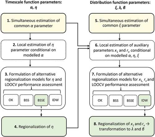
The workflow of the methodology is presented in Fig. 2.

Figure 2. Workflow of the regionalization procedure. Yellow boxes correspond to procedures for simultaneous parameter estimation (shared parameters), green ones correspond to the final regionalization procedures and the remaining white boxes denote procedures that are intermediate and auxiliary to the regionalization.

3.3 At-site deviations metrics

After the regionalization procedure, we aim to evaluate the deviations between the regionalized model estimates and the empirical rainfall quantiles. To investigate the impact of the regionalization on estimation for different return periods, we also estimate the deviations between the local (at-site) independently fitted parameters and the ones obtained after the regionalization. The following three deviation statistics are used for each scale:

1. The dimensionless (%) mean deviation of the model from the empirical K-moments, for a given time scale $\mathit{k}$:

(10) ${{\mathit{D}}_{\mathrm{a}}}^{\left(\mathit{k}\right)}:=\frac{100}{n_k}\sum _{\mathit{p}=1}^{n_k}\frac{x_{T_p}^{\left(\mathit{k}\right)}-{{\hat{K}}_{\mathit{p}}^{\prime }}^{\left(\mathit{k}\right)}}{{{\hat{K}}_{\mathit{p}}^{\prime }}^{\left(\mathit{k}\right)}}$(10)

where ${\hat{K}}_{\mathit{p}}^{\prime }$ is the empirical K-moment of order $\mathit{p}$ corresponding to return period $T_p$, $n_k$ is the data length for the given time scale, and $x_{T_p}$ is the model-derived rainfall intensity corresponding to the same return period $T_p$. The methodology to assign return periods to the empirical K-moments is detailed in the companion paper (Koutsoyiannis et al. 2024).

• (2) The dimensionless (%) RMSE of the model estimates from the empirical K-moments, for a given time scale $\mathit{k}$:

(11) $\mathrm{RMS}{\mathrm{E}}^{\left(\mathit{k}\right)}=\frac{100}{{{\hat{K}}^{\prime }}_{p_{\mathrm{avg}}}^{\left(\mathit{k}\right)}}\sqrt{\frac{1}{n_k}\sum _{\mathit{p}=1}^{n_k}{\left(x_{T_p}^{\left(\mathit{k}\right)}-{{\hat{K}}^{\prime }}_{\mathit{p}}^{\left(\mathit{k}\right)}\right)}^2}$(11)

where ${{\hat{K}}^{\prime }}_{p_{\text{avg}}}\left(\mathit{k}\right)$ the average of the empirical K-moments for the given time scale, which is used to standardize and compare the RMSE of the different time scales.

• (3) The dimensionless (%) deviation of the regional model from the local model:

(12) ${{\mathit{D}}_{\mathrm{r}}}^{\left(\mathit{k},\mathit{T}\right)}:=100\frac{\left({\mathit{x}}_{\mathit{T}{,}_{\mathrm{reg}}}^{\left(\mathit{k}\right)}-x_{\mathit{T}{,}_{\mathrm{point}}}^{\left(\mathit{k}\right)}\right)\times 2}{x_{\mathit{T}{,}_{\mathrm{reg}}}^{\left(\mathit{k}\right)}+x_{\mathit{T}{,}_{\mathrm{point}}}^{\left(\mathit{k}\right)}}$(12)

where $x_{\mathit{T}{,}_{\mathrm{reg}}}^{\left(\mathit{k}\right)}$ and $x_{\mathit{T}{,}_{\mathrm{point}}}^{\left(\mathit{k}\right)}$ are the regional and at-site (point) model estimate for a given scale $\mathit{k}$ and return period $\mathit{T}$. The $D_{\mathrm{r}}$ is estimated only for the set of the sub-daily raingauges since they allow full calibration of the ombrian relationships prior to regionalization (in contrast to the daily raingauges for which the parameters of the time scale function cannot be determined beforehand).

4 Results and analysis

4.1 Regionalization of parameters of the time scale function

4.1.1 Parameter α

From the preliminary point estimation of the parameters of the time scale function, we found that the estimation of the parameter $\mathit{\alpha }$ greatly depends on the temporal resolution of the measuring instrument, as shown in Fig. A1 and A2 in Appendix A. Specifically, in stations with fine temporal resolution (5 or 10 min) the resulting values of parameter $\mathit{\alpha }$ were small – and vice versa. This is interpreted as an artificial statistical effect rather than representing some physical reality. To compensate for the sensitivity of the α parameter to time resolution of the data, we identified a single value of this parameter for Greece, by the following procedure:

1. We selected the 53 stations with the longest records having temporal resolution of 30 min or finer, distributed over all 14 water districts.

2. We re-estimated the parameters of the equation $\mathit{a}\left(\mathit{k}\right)$, α and η, through optimization in which we set as a constraint that the value of the α parameter is the same among all 53 stations, while the $\mathit{\eta }$ value was allowed to vary.

As a result of this optimization, the common value of α = 0.18 h is obtained and used in all further analyses.

4.1.2 Parameter η

Conditional on the common α parameter, $\mathit{\alpha }=0.18$ h, the η parameter is re-estimated for all stations with sub-daily resolution. The four spatial models, BSS, BSSE, IDW and OK, are fitted to the point estimates and results are evaluated through multiple error metrics for the entire dataset and for the LOOCV analysis, as shown in Table 3 and Table 4, respectively. As explained in Section ‎3.2.3, the best model is chosen based on the LOOCV analysis, which in this case favours the BSSE model, having as an additional explanatory variable the elevation. In particular, an inverse relationship of $\mathit{\eta }$ with the altitude is identified, i.e. lower (higher) values of the parameter are more likely at high (low) altitudes, as seen in Fig. 3.

Figure 3. Regionalized η parameter resulting from the application of the BSSE model. The coordinate reference system is the GGRS87/Greek Grid (EPSG:2100).

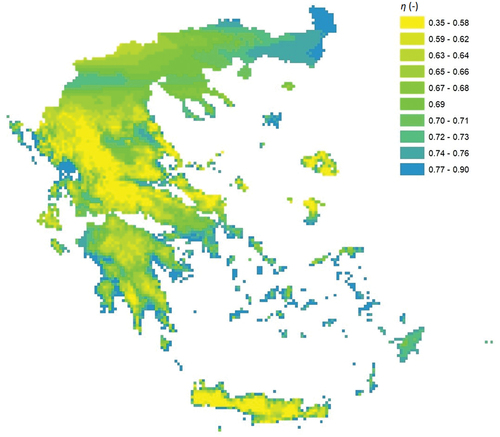
Table 3. Entire dataset statistics for η, x₁ and $r_x$.

Interpolation method	MBE	MAE	RMSE	R^2	EF
η
BSS	0.00	0.07	0.08	0.25	0.26
BSSE*	0.00	0.05	0.06	0.57	0.57
OK	0.00	0.03	0.03	0.91	0.88
IDW	0.00	0.01	0.02	0.98	0.98
x1
BSS	0.00	0.02	0.04	0.28	0.27
BSSE	0.00	0.38	0.54	0.63	0.43
OK	0.00	0.21	0.31	0.90	0.88
IDW*	0.01	0.13	0.24	0.93	0.92
$r_x$
BSS	0.00	0.17	0.26	0.26	0.20
BSSE	0.00	0.18	0.26	0.27	0.26
OK	0.00	0.15	0.23	0.38	0.33
IDW*	0.01	0.13	0.24	0.93	0.92

*denotes best performance according to LOOCV.

Table 4. Leave-one-out cross-validation statistics for η, x₁ and $r_x$.

Interpolation method	MBE	MAE	RMSE	R^2	EF
η
BSS	0.00	0.07	0.08	0.28	0.28
BSSE*	0.00	0.06	0.07	0.40	0.40
OK	0.00	0.07	0.08	0.30	0.28
IDW	0.00	0.06	0.08	0.28	0.28
x1
BSS	0.00	0.02	0.04	0.18	0.17
BSSE	–0.01	0.51	0.75	0.43	0.40
OK	0.00	0.43	0.64	0.49	0.47
IDW*	0.01	0.44	0.65	0.49	0.48
$r_x$
BSS	0.00	0.18	0.27	0.16	0.12
BSSE	0.00	0.18	0.27	0.18	0.15
OK	0.00	0.18	0.28	0.08	0.07
IDW*	–0.01	0.17	0.29	0.32	0.28

*denotes best performance according to LOOCV.

4.2 Regionalization of parameters of the distribution function

4.2.1 Tail-index ξ

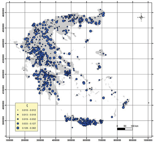
In the preliminary point investigation of the parameter variability, the parameter ξ (tail index of the distribution) is estimated individually per station and per instrument, and simultaneously with the optimization of the other parameters of the ombrian curves. As expected, a large spatial variability of the parameter estimates is obtained (Fig. A3 in Appendix A), which indicates both the measurement uncertainty of maximum rainfall and the estimation uncertainty due to varying record lengths of the employed stations. To assess whether this variability might also reflect physically reasoned patterns in the regional realization of extreme rainfall, we perform the following investigations.

We form two datasets: (a) one comprising 61 daily raingauge stations which have at least 60 years of complete daily time series (termed complete daily long dataset, CDLD) and (b) a second one comprising 147 stations across the Greek territory which have at least 60 years of annual maxima values (termed annual maxima long dataset, AMLD) and which can support the estimation of the parameter with greater reliability. Using the CDLD, we attempt to link the variability of the tail index with (i) elevation, (ii) average daily rainfall, (iii) wet-day average daily rainfall and (iv) the average of the n largest rainfall depths, where n is the number of years. To reduce the uncertainty, we condition the β parameter to represent the probability dry estimated from the daily series (see Koutsoyiannis et al. 2024) and allow only $\mathit{\xi }$ and $\mathit{\lambda }$ to vary. We find:

1. a weak negative correlation with elevation, explaining only 9% of the variance,

2. a moderate positive correlation with the inverse of average daily rainfall, explaining 28% of the variance,

3. a moderate positive correlation with the inverse of the wet-day average daily rainfall, explaining 31% of the variance, and

4. a weak correlation with the average of the n largest rainfall depths, explaining 18% of the variance of the estimates.

It is thus deemed that only cases (ii) and (iii) might be useful for the estimation of the parameter, with case (ii) being practically superior because information for the average daily rainfall is already available in a grid produced by the BSSE method (Koutsoyiannis et al. 2023b).

We attempt to reproduce analysis (ii) using the AMLD dataset, thus making the estimation based only on annual maxima data and extracting the average daily rainfall information from the BSSE model grid, since otherwise this covariate should be estimated from complete daily series. In this case, we observed (not shown) that although the tail index estimates from the two datasets retained a satisfactory match (y = 0.88x, R² = 0.79), the correlation with the average daily rainfall weakened dramatically with respect to the CDLD analysis and the explained variance decreased to zero. Considering the above results and the data limitations, we conclude that there is no strong basis to model the tail index estimated from the annual maxima dataset employing other available explanatory variables, representing a physical regime.

We continue the investigation by assuming that the entire variability of ξ estimates is a statistical effect. Making this assumption, we can unify (merge) all CDLD records at a certain time scale after standardizing with the mean, and we estimate a unique value of ξ from the unified record comprising 299 481 (standardized) non-zero daily rainfall values (the value of 0.1 mm is used as the threshold for a wet day). We fit the Pareto distribution, which in preliminary analyses proved to be a good model for non-zero daily rainfall, using the method of K-moments. 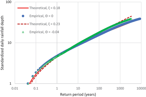Parameters $\mathit{\lambda }$ and $\mathit{\xi }$ are estimated conditional on a fixed $\mathit{\beta }$ parameter which is in turn estimated based on the probability wet (see Koutsoyiannis et al. 2024). For this estimation (which is based on the unified full daily records), we exclude the record’s largest K-moment to avoid potential outlier effects, and we also exclude the K-moments which are lower than the mean value of the unified record, to make the estimation more focused on larger events. The resulting ξ is estimated to be 0.18 if the different stations are assumed independent (Θ = 0) or larger if dependence is assumed (ξ = 0.23 for Θ = −0.04, where Θ denotes bias; see Koutsoyiannis et al. 2024 for details), as shown in Fig. 4. The lower value ξ = 0.18 is finally chosen.

Figure 4. Theoretical (Pareto) and empirical distribution of the standardized daily rainfall depth for the case where dependence bias is considered ($\mathrm{\Theta }$ = −0.04) and the case where dependence is neglected ($\mathrm{\Theta }$ = 0).

To validate the assumption of a common ξ parameter, we perform the following six Monte Carlo scenarios, in each of which we produce 70 simulations with 70 values from the Pareto distribution. In the first three we assume a ξ value of 0.18 and in the rest 0.01, while the λ value is 1 for all cases. The scenarios are generated based on the following three assumptions:

1. For each series, the 70 values are generated from the unbounded Pareto distribution, P(λ,ξ).

2. For each series, the 70 values are assumed to constitute the upper c = 20% of a larger sample (350 values) which is generated from the conditional Pareto distribution P(λ,ξ,c).

3. For each series, the 70 values are assumed to constitute the upper c = 2% of a larger sample (3500 values) which is generated from the conditional Pareto distribution P(λ,ξ,c).

The third assumption is more representative of the historical data and is also the one yielding the smallest uncertainty among the three; relevant results are shown in Fig. 5 and Fig. 6. The findings show the (expected) large variability of the estimates in the case of a large tail index, even for the third case. Specifically, when the true value is 0.01 the estimates span from −0.13 to 0.14, but the respective variability of the estimated value of ξ (ξ_e) spans from ~ −0.1 to ~0.5 when the true value is ξ = 0.18. This finding supports the consistency of the assumption of a single ξ = 0.18 for the entire Greek territory, which is kept for the rest of the analysis.

Figure 5. Probability distribution of simulated tail index ξ_e, generated from a Pareto distribution with scale parameter λ = 1 and theoretical tail index ξ = 0.01 and ξ = 0.18 assuming that the generated values are the upper 2% of a larger sample. The results are obtained from 70 simulated series of 70 values, for each of which the empirical values λ_e and ξ_e are estimated by optimization. In addition to the empirical distributions, the theoretical normal distributions N(ξ – ζ, σ) are also shown, where ζ = −0.03 is the bias and σ the standard deviation, with values as in the legend of the figure, both estimated with Monte Carlo.

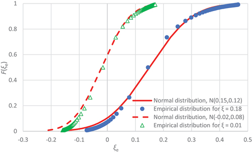
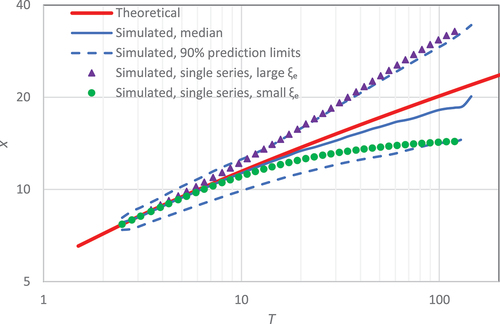
Figure 6. Probability distribution of simulated standardized daily rainfall, generated from a Pareto distribution with scale parameter λ = 1 and tail index ξ = 0.18 assuming that the simulated values are the upper 2% of a larger sample. In addition to the median and 90% confidence limits of the simulated empirical distributions, two individual simulated distributions are shown with an empirical (optimized) index ξ_e approximately equal to its upper and lower confidence limits (where the high and low ξ_e are 0.35 and −0.02, respectively).

4.2.2 Parameters β and λ

At this step, we estimate the final two parameters $x_1$ and $r_x$ (to be transformed into β and λ), conditional on the previously estimated α, η and ξ parameters. 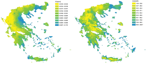These are estimated as the theoretical rainfall intensities $x_1$ corresponding to return periods ${\mathit{T}}_1$= 2 years and $\mathit{k}$ =24 h and the ratio of intensities $r_x:=x_2/x_1$, where $x_2$ the theoretical intensity corresponding to ${\mathit{T}}_2$= 100 years and $\mathit{k}$ = 24 h. The spatial models are fitted independently to the auxiliary parameters and the results evaluated as in the case of the η parameter are shown in Table 3 and Table 4. In this case, both evaluations favour the IDW model, which is applied for both parameters. After the regionalization, the grids are transformed (via Equation (5)) into the original parameters β and λ, the geographic distribution of which is shown in Fig. 7.

Figure 7. Regionalized β (years) and λ (mm/h) parameters using the IDW method. The coordinate reference system is the GGRS87/Greek Grid (EPSG:2100).

4.3 Performance assessment

4.3.1 Regionalization models

Table 3 and Table 4 summarize the regionalization performance for the three spatially varying parameters η, x₁ and r_x, in terms of the statistics calculated for the entire dataset and the ones calculated based on the LOOCV, respectively. It is recalled that the best regionalization method per parameter is chosen as the one showing superior performance in LOOCV mode, as this is a better index of its performance in pragmatic design conditions, in which ungauged areas are more likely. Expectedly, results as per the best model may differ in these two evaluations, i.e. for the η parameter the BSSE model does not show the best performance when the entire dataset is used, yet it is superior in LOOCV evaluation. The latter is an indication of the increased uncertainty involved in the regionalization of this parameter, which is based on records with sub-daily resolution. On the other hand, the IDW is consistently selected as the best model for the x₁ and r_x parameters in both evaluations. The superiority of the IDW method may be surprising given its simplicity and the exactness of the interpolation, but these aspects make it superior in the frame of the sequential order of the regional scheme, having previously incorporated smoothing schemes. We note that the regionalization of the x₁ and r_x parameters is performed simultaneously at the end of the regionalization process, after the choice of two common parameters and one regionally varying one derived by the BSSE smoothing method. Therefore, a considerable amount of smoothing has been implemented in the conditional point estimates, and hence the more exact IDW method, preserving the local effects, is selected to compensate for the existing smoothing effect and retain a greater degree of accuracy in the final estimates.

The inter-comparison of the BSS and the BSSE performance, with the latter employing elevation as an additional covariate, allows us to also evaluate the impact of orography in an objective manner. It is seen that elevation is useful as a covariate both for the η parameter (in this case the BSSE is also the best-performing model), and in the case of the x₁ parameter which stands for a low (2-year) return period estimate of rainfall intensity. On the other hand, the amelioration of the $r_x$ regionalization after the inclusion of elevation information is minor, which suggests that elevation is less informative in the case of an extremeness ratio (it is recalled that $r_x$ is the ratio of the 100-year return period estimate to the 2-year one).

It is noted that Tables 3 and 4 report the global error statistics, while the spatial distribution thereof was also visually checked, and no systematic errors were identified over Greece. However, a few higher errors in the regionalization of the η parameter (controlling the time scale function of the ombrian curves) were identified in orographically complex areas, exhibiting various and abrupt changes in elevation. These may indicate local orographic effects which are difficult to capture given the sparse resolution of the sub-daily raingauges, which are used for the regionalization of the η parameter.

4.3.2 At-site deviations of rainfall quantiles

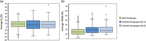
To evaluate the performance of the regionalization with respect to the at-site rainfall quantiles, we estimate the deviations of the regional model estimates from the empirical values for all stations, daily and sub-daily. The latter are statistically evaluated according to the metrics defined in Section ‎3.3, based on the K-moments framework. The average deviation over all time scales is shown (Figure 8) separately for the daily raingauges (averaged over the 24 h and 48 h scales) and the sub-daily raingauges (averaged over all available scales), also differentiating between those at unique locations used for the calibration of all parameters (Set A) and those that were at the same location with a daily raingauge, which was preferred for the calibration of the distribution function (Set B). It is observed that the distribution of average deviation is slightly biased towards positive values (due to the correction of the shape parameter in the regional model, see also investigation in Section 4.2.1 and Discussion) with the median being 8.14% for the daily raingauges, 5.6% for Set A and 6.19% for Set B, while the median of the average RMSE is 14.51% for the daily raingauges, 18.67% for Set A and 17.56% for Set B. Interestingly, a similarly good performance is obtained for Set B, which acts as a validation set, since these records were not used for the calibration of the distribution function, but only for the estimation of the parameters of the time scale function. Detailed results for all time scales are shown in Appendix B (Fig. B1 and B2), suggesting the increased uncertainty prevalent at the small time scales – for which, however, fewer records are available (Table 1).

Figure 8. Dimensionless (%) mean deviation of the model from the empirical K-moments (a) and dimensionless (%) RMSE (b), both averaged over all time scales available from the daily and sub-daily raingauges. Set A indicates the sub-daily raingauges used for the full calibration of the ombrian relationships, while Set B denotes the sub-daily raingauges used only for the calibration of the parameters of the time scale function.

To inspect the impact of regionalization on design rainfall estimates for various return periods, we compare the deviations between the estimates using the regional parameters and the ones obtained using the local (at-site) parameters estimated only from the set of sub-daily raingauges (see Section 3.3.), shown for two characteristic scales in Fig. 9.

Figure 9. Dimensionless (%) deviation of the regional model from the local model (estimated from the set of sub-daily raingauges) for 1 h scale (a) and 24 h scale (b) and different return periods.

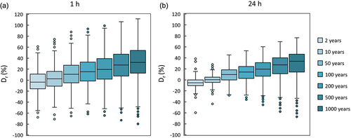
For both scales, the deviations consistently tend to increase towards larger values as the return period increases. This is attributed to the use of the single high value of the parameter ξ in the regionalization (estimated from the high-quality set of long daily raingauges, see Section 4.2.1), the influence of which is stronger in high return periods (for T = 1000 years, median 32.35% at 1 h and 33.86% at 24 h). In the low return periods (of the order of 2 years), the spatially generalized rainfall model leads to slightly smaller rainfall estimates (for T = 2 years, median −3.55% at 1 h and −5.22% at 24 h).

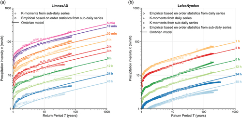
An illustration of the fitting is shown in Fig. 10 for two stations: Limnos, a station with only sub-daily data at a single location (example of Set A); and Lofos Nymfon (Hill of Nymphs), a station with two gauges, a daily raingauge used for the calibration of the distribution function and a sub-daily raingauge used for the calibration of the time scale function (an example of Set B). It is noted that the daily raingauge at the Lofos Nymfon is also the longest rainfall record available in Greece (dating back to 1863).

Figure 10. Theoretical and empirical distributions of annual maximum intensities at scales of 5 min to 48 h (depending on the available samples) from the sub-daily stations of Limnos (a) and Lofos Nymphon-Athens (b). For the latter, the empirical intensities at the 24 h and 48 h scales from the daily raingauge are shown as well. The empirical intensities plotted based on order statistics are also shown for validation.

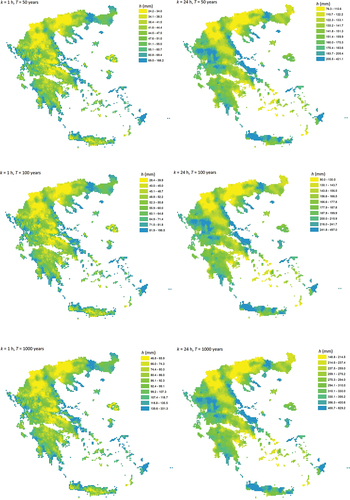
4.4 Design rainfall maps

The design rainfall (in mm) maps for scales of 1 and 24 h are shown in Fig. 11 for return periods T = 50, 100 and 1000 years. The emerging spatial patterns are consistent with known Greek climatology, namely the impact of orography and the increased spatial diversity, with lower amounts of rainfall occurring in eastern Greece compared to its western counterpart, except for some coastal areas in eastern Greece, in which rainfall rates are very intense. Geographic patterns are more abrupt at the 1 h scale, reflecting the erratic nature of fine-scale precipitation, whereas patterns are smoother over the 24 h scale and in accordance with the orographic effect, i.e. higher rainfall amounts at the daily scale are more likely in the mountainous regions. On the other hand, the orographic enhancement of precipitation is not evident at the 1 h scale; rather, the rainfall depths appear decreased in some regions with higher elevations (namely along the Pindus Mountain range) compared to lower elevation/coastal areas.

Figure 11. Left panel: estimated rainfall depth (mm) for 1 h and return periods 50, 100 and 1000 years, right panel: estimated rainfall depth (mm) for 24 h and return periods 50, 100 and 1000 years. Quantile classification is employed for all legends. The coordinate reference system is the GGRS87/Greek Grid (EPSG:2100).

5 Discussion

The large-scale regionalization scheme employed herein entails several methodological choices that warrant further discussion, aside from the discussion of the findings.

A critical choice, stemming from a thorough physically reasoned and stochastic investigation of the longest high-quality records (Section 4.2.1), is the implementation of a common tail-index (parameter $\mathit{\xi }$) over Greece. In the absence of robust geographic and hydroclimatic links, this choice is dictated by the substantial uncertainty involved in the estimation of the tail index, which is particularly relevant given the limited record lengths available (Koutsoyiannis 2004). This uncertainty is re-estimated herein by means of Monte Carlo simulations and found consistent with the observed variability of the (at-site) point estimates. It is noted that the alternative approach of independent estimation and interpolation of the ξ parameters, despite being simple, is likely to result in unrealistic spatial patterns and abrupt changes, as already shown by Uboldi et al. (2014) and Jalbert et al. (2022). On the other hand, a spatially invariant tail-index is a widely used approach in regionalization of extreme rainfall (see e.g. Jalbert et al. 2022), even used in the global-scale investigation of IDF curves by Courty et al. (2019). Shehu et al. (2023), in the regionalization of the curves for Germany, also concluded on keeping the tail-index constant, and simultaneously regionalizing the rest of the parameters using kriging methods. As a result of the common and high tail index, the regional model’s predictions, for the higher return periods, tend to be greater than the single-station rainfall quantiles, as well as the single-site (independently estimated) model predictions. This is to be expected as the pooling methodology (Section 4.2.1) used for the estimation of the tail-index in the regional model aimed in the first place to compensate for the underestimation bias of the tail-index due to the small sample size of the individual records.

Another finding worth discussing is the inclusion of the IDW method in the regionalization framework, which demonstrated its superiority in the case of the x₁ and $r_x$ parameters. Bloeschl and Grayson (2001) showed that the IDW generates spurious artefacts in the case of highly variable quantities and irregularly spaced data sites. We also deem that this would be true had we applied IDW as the primary regionalization method. Yet by applying this method at the end of the sequential regionalization, we have already smoothed out a significant degree of variation, and at that point of the regionalization process, greater precision is a desired fact. Indeed, the resulting patterns are relatively smooth and can be efficiently interpolated by a simpler method. This is the reason why IDW is often part of hybrid approaches (e.g. Perica et al. 2009) and even sophisticated algorithms incorporate some sort of IDW (e.g. PRISM, Daly 2006). It is also important to consider that the superiority of no method is guaranteed under general conditions. For instance, recently, Sangüesa et al. (2023) suggested that IDW outperformed kriging in the case of sparse data.

Finally, the usefulness of elevation as a geographic covariate for extreme rainfall is an open research question, with various methodologies and regions reporting diverse results. For instance, Szolgay et al. (2009) did not find elevation significant as an additional explanatory variable for 2- and 100-year daily rainfall depths in Central Slovakia. In contrast, regional rainfall studies in Greece at smaller spatial scales (e.g. Iliopoulou and Koutsoyiannis 2022, Iliopoulou et al. 2022) identified elevation as a good explanatory variable mainly affecting the mean of the annual maxima distribution at the daily scale. Here, elevation is found useful for the regionalization of the η parameter (controlling the scaling of the intensity) and to a lesser extent found meaningful for the 2-year daily rainfall intensity (although this model did not rank best). Resulting maps (Section ‎4.4) suggest that orography enhances precipitation at the 24 h scale, but this effect is not evident at the 1 h scale; instead, a tendency for intensity to drop with elevation at the short time scales is identified for some regions. Therefore, the dependence of rainfall intensity on elevation is not uniform even across scales. Similar results have been reported for Italy (see e.g. Mazzoglio et al. 2022), where a decrease of annual maxima 1 h rainfall with elevation has been identified and called a “reverse orographic effect” (Avanzi et al. 2015). More research is required, however, to disentangle the effect of elevation across the different scales and to investigate the usefulness of other proxies of the rainfall generating mechanisms (e.g. convection) into the regionalization of the parameters.

6 Conclusions

In this work, we have developed a sequential regionalization methodology for design rainfall in the form of rainfall intensity–time scale–return period relationships and applied the latter over the entire Greek territory (131 957 km²). This is the first time a regional design rainfall model has been available in gridded form (in a 5 km × 5 km grid) for Greece. The approach followed incorporates an advanced framework for regional probability analysis employing knowable (K-) moments and a more physically sound re-parameterization of the Koutsoyiannis et al. (1998) model. The theoretical background is extensively discussed in the companion paper by Koutsoyiannis et al. (2024), whereas the regional implementation and the results are presented herein.

The regionalization process was informed by extensive analyses using the independent, at-site estimation results as a basis. Via comprehensive evaluations of the variability involved in the estimation of the parameters, two parameters were considered spatially invariant, i.e. the time scale parameter $\mathit{\alpha }$ and the tail-index $\mathit{\xi }$, and were estimated simultaneously employing the longest high-quality records, in order to increase the robustness of the estimation. The calibration of the tail index has been corroborated by extensive stochastic investigations. The other three parameters ($\mathit{\eta }$, $\mathit{\lambda }$ and $\mathit{\beta }$) were regionalized following a sequential implementation scheme that exploits information from both daily and sub-daily raingauges. In particular, by first regionalizing the parameters of the time scale function from the sub-daily raingauges, the methodology allows an efficient incorporation of the denser and more reliable network of daily raingauges for the subsequent calibration of the distribution function. Four regionalization methods, ranging from smoothing to exact interpolation schemes, namely the BSS, BSSE, OK and IDW, were applied and evaluated for each of the three parameters, while the impact of elevation was also considered. The best method was selected per parameter in terms of the LOOCV performance, and a final hybrid scheme emerged that combines smoothing and exact interpolation techniques. In particular, the BSSE smoothing method with the altitude as explanatory variable was selected for the regionalization of the $\mathit{\eta }$ parameter of the time scale function, performed first, while the exact IDW was selected for the remaining two parameters, $\mathit{\lambda }$ and $\mathit{\beta }$, the regionalization of which was performed at the end of the sequential procedure. Therefore, the framework allowed the evaluation of the necessary degree of smoothing at each step of the sequential regionalization based on the cross-validation performance.

The final product consists of a five-parameter relationship, with two constant parameters and three spatially varying parameters available in a 5 km ×5 km grid. This forms a powerful and easy to apply design tool covering the entire territory of Greece, while the methodology can be readily transferred to other countries or parts thereof.

Acknowledgements

We are grateful to Associate Editor Elena Volpi, as well as to Professor Pierluigi Claps and a second (anonymous) reviewer, for their comments which helped us to improve the manuscript.

Disclosure statement

No potential conflict of interest was reported by the author(s).

Data availability statement

The data of the General Directorate of Water of the Greek Ministry of Environment and Energy are available online for free from the Hydroscope platform (http://www.hydroscope.gr/, accessed 25 March 2023). All other data belong to other Greek organizations and are not publicly available.

Additional information

Funding

This research was funded by the General Directorate of Water of the Greek Ministry of Environment and Energy through the unit “Eπιτελική ∆oμή EΣΠA Υπoυργείoυ Περιβάλλoντoς και Eνέργειας Toμέα Περιβάλλoντoς” in the framework of the project “Production of maps with updated parameters of the ombrian curves at country level (implementation of the EU Directive 2007/60/EC in Greece).”

Appendix

Appendix A: Results from point investigation

Figure A1. Estimate of parameter $\mathit{\alpha }$ vs temporal resolution of the rain recorder.

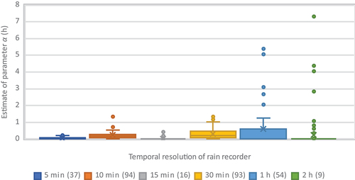
Figure A2. Average of estimated $\mathit{\alpha }$ parameters vs the temporal resolution of the rain recorders.

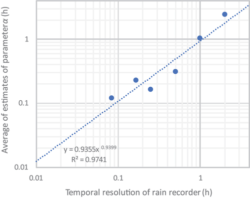
Figure A3. Geographic distribution of the independently estimated ξ parameters.

Appendix B:

Supplementary results from regionalization

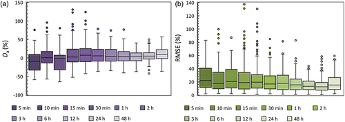
Figure B1. Dimensionless (%) mean deviation of the model from the empirical K-moments (a) and dimensionless (%) root mean square error (RMSE, (b)), for all time scales available from the daily raingauges.

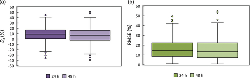
Figure B2. Dimensionless (%) mean deviation of the model from the empirical K-moments (a) and dimensionless (%) RMSE (b), for all time scales available from the sub-daily raingauges.

References

- Ahrens, B., 2006. Distance in spatial interpolation of daily rain gauge data. Hydrology and Earth System Sciences, 10 (2), 197–208. doi:10.5194/hess-10-197-2006.
- Aron, G., et al. 1987. Regional Rainfall intensity‐duration‐frequency curves for Pennsylvania 1. Journal of the American Water Resources Association, 23 (3), 479–485. doi:10.1111/j.1752-1688.1987.tb00826.x.
- Avanzi, F., et al. 2015. Orographic signature on extreme precipitation of short durations. Journal of Hydrometeorology, 16 (1), 278–294. doi:10.1175/JHM-D-14-0063.1.
- Barbosa, A.D.G., et al. 2022. Assessing intensity-duration-frequency equations and spatialization techniques across the Grande River Basin in the state of Bahia, Brazil. RBRH, 27.
- Bernard, M.M., 1932. Formulas for rainfall intensities of long duration. Transactions of the American Society of Civil Engineers, 96 (1), 592–606. doi:10.1061/TACEAT.0004323.
- Blanchet, J., et al. 2016. A regional GEV scale-invariant framework for intensity–duration–frequency analysis. Journal of Hydrology, 540, 82–95. doi:10.1016/j.jhydrol.2016.06.007.
- Blöschl, G. and Grayson, R., 2001. Spatial observations and interpolation. In: R. Grayson and G. Blöschl, eds. Spatial patterns in catchment hydrology. Cambridge, UK: Cambridge University Press, 17–50.
- Bohling, G., 2005. Introduction to geostatistics and variogram analysis. Kansas Geological Survey, 1 (10), 1–20.
- Burlando, P. and Rosso, R., 1996. Scaling and muitiscaling models of depth-duration-frequency curves for storm precipitation. Journal of Hydrology, 187 (1–2), 45–64. doi:10.1016/S0022-1694(96)03086-7.
- Burn, D.H., 2014. A framework for regional estimation of intensity–duration–frequency (IDF) curves. Hydrological Processes, 28 (14), 4209–4218. doi:10.1002/hyp.10231.
- Burrough, P.A., McDonnell, R.A., and Lloyd, C.D., 2015. Principles of geographical information systems. USA: Oxford University Press.
- Cassalho, F., et al. 2019. Artificial intelligence for identifying hydrologically homogeneous regions: a state‐of‐the‐art regional flood frequency analysis. Hydrological Processes, 33 (7), 1101–1116. doi:10.1002/hyp.13388.
- Ceresetti, D., et al. 2012. Evaluation of classical spatial-analysis schemes of extreme rainfall. Natural Hazards and Earth System Sciences, 12 (11), 3229–3240. doi:10.5194/nhess-12-3229-2012.
- Claps, P., Ganora, D., and Mazzoglio, P., 2022. Rainfall regionalization techniques. In: R. Morbidelli, ed. Rainfall. Elsevier, 327–350. doi:10.1016/B978-0-12-822544-8.00013-5.
- Courty, L.G., et al. 2019. Intensity-duration-frequency curves at the global scale. Environmental Research Letters, 14 (8), 084045. doi:10.1088/1748-9326/ab370a.
- Daly, C., 2006. Guidelines for assessing the suitability of spatial climate data sets. International Journal of Climatology: A Journal of the Royal Meteorological Society, 26 (6), 707–721. doi:10.1002/joc.1322.
- Deidda, R., Hellies, M., and Langousis, A., 2021. A critical analysis of the shortcomings in spatial frequency analysis of rainfall extremes based on homogeneous regions and a comparison with a hierarchical boundaryless approach. Stochastic Environmental Research and Risk Assessment, 35 (12), 2605–2628. doi:10.1007/s00477-021-02008-x.
- De Luca, D.L. and Napolitano, F., 2023. A user-friendly software for modelling extreme values: EXTRASTAR (EXTRemes Abacus for STAtistical Regionalization). Environmental Modelling and Software, 161, 105622. doi:10.1016/j.envsoft.2023.105622.
- Faulkner, D.S. and Prudhomme, C., 1998. Mapping an index of extreme rainfall across the UK. Hydrology and Earth System Sciences, 2 (2/3), 183–194. doi:10.5194/hess-2-183-1998.
- Forestieri, A., et al. 2018. Regional frequency analysis of extreme rainfall in Sicily (Italy). International Journal of Climatology, 38, e698–e716. doi:10.1002/joc.5400.
- Goovaerts, P., 1997. Geostatistics for natural resources evaluation. New York: Oxford University Press.
- Goovaerts, P., 2000. Geostatistical approaches for incorporating elevation into the spatial interpolation of rainfall. Journal of Hydrology, 228 (1–2), 113–129. doi:10.1016/S0022-1694(00)00144-X.
- Hailegeorgis, T.T., Thorolfsson, S.T., and Alfredsen, K., 2013. Regional frequency analysis of extreme precipitation with consideration of uncertainties to update IDF curves for the city of Trondheim. Journal of Hydrology, 498, 305–318. doi:10.1016/j.jhydrol.2013.06.019.
- Haruna, A., Blanchet, J., and Favre, A.C., 2023. Modeling intensity‐duration‐frequency curves for the whole range of non‐zero precipitation: a comparison of models. Water Resources Research, 59 (6), e2022WR033362. doi:10.1029/2022WR033362.
- Hengl, T., 2006. Finding the right pixel size. Computers & Geosciences, 32 (9), 1283–1298. doi:10.1016/j.cageo.2005.11.008.
- Hosking, J.R.M. and Wallis, J.R., 1997. Regional frequency analysis.
- Huffman, G.J., et al. 2019. GPM IMERG final precipitation L3 half hourly 0.1 degree x 0.1 degree V06. Greenbelt, MD: Goddard Earth Sciences Data and Information Services Center (GES DISC). doi:10.5067/GPM/IMERG/3B-HH/06.
- Hutchinson, M.F., 1995. Interpolating mean rainfall using thin plate smoothing splines. International Journal of Geographical Information Systems, 9 (4), 385–403. doi:10.1080/02693799508902045.
- Iliopoulou, T., et al. 2023. Regionalized design rainfall curves for Greece ( No. EGU23-8740). Copernicus Meetings.
- Iliopoulou, T. and Koutsoyiannis, D. 2022. A parsimonious approach for regional design rainfall estimation: the case study of Athens. In: Proceedings of 7th IAHR Europe Congress “Innovative Water Management in a Changing Climate” Athens: International Association for Hydro-Environment Engineering and Research (IAHR).
- Iliopoulou, T., Malamos, N., and Koutsoyiannis, D., 2022. Regional ombrian curves: design rainfall estimation for a spatially diverse rainfall regime. Hydrology, 9 (5), 67. doi:10.3390/hydrology9050067.
- Jalbert, J., Genest, C., and Perreault, L., 2022. Interpolation of precipitation extremes on a large domain toward idf curve construction at unmonitored locations. Journal of Agricultural, Biological and Environmental Statistics, 27 (3), 461–486. doi:10.1007/s13253-022-00491-5.
- Jarvis, A., et al. 2008. Hole-filled SRTM for the globe Version 4. Available from the CGIAR-CSI SRTM 90m Database. http://srtm.csi.cgiar.org [Accessed 01 Sep 2022].
- Koutsoyiannis, D., 2004. Statistics of extremes and estimation of extreme rainfall: i. Theoretical investigation/Statistiques de valeurs extrêmes et estimation de précipitations extrêmes: i. Recherche théorique. Hydrological Sciences Journal, 49 (4), 590.
- Koutsoyiannis, D., 2019. Knowable moments for high-order stochastic characterization and modelling of hydrological processes. Hydrological Sciences Journal, 64 (1), 19–33. doi:10.1080/02626667.2018.1556794.
- Koutsoyiannis, D., 2023. Stochastics of hydroclimatic extremes - a cool look at risk. 3ed. Athens: Kallipos Open Academic Editions.
- Koutsoyiannis, D., et al. 2023a. Technical report, production of maps with updated parameters of the ombrian curves at country level (implementation of the EU directive 2007/60/EC in Greece). Department of Water Resources and Environmental Engineering – National Technical University of Athens.
- Koutsoyiannis, D., et al. 2023b. In search of climate crisis in Greece using hydrological data: 404 not found. Water, 15 (9), 1711. doi:10.3390/w15091711.
- Koutsoyiannis, D., et al., 2024. A stochastic framework for rainfall intensity–timescale–return period relationships. Part I: theory and estimation strategies. Hydrological Sciences Journal. doi:10.1080/02626667.2024.2345813
- Koutsoyiannis, D. and Iliopoulou, T., 2022. Ombrian curves advanced to stochastic modeling of rainfall intensity. In: R. Morbidelli, ed. Rainfall. Elsevier, 261–284. doi:10.1016/B978-0-12-822544-8.00003-2.
- Koutsoyiannis, D., Kozonis, D., and Manetas, A., 1998. A mathematical framework for studying rainfall intensity-duration-frequency relationships. Journal of Hydrology, 206 (1–2), 118–135. doi:10.1016/S0022-1694(98)00097-3.
- Koutsoyiannis, D. and Papalexiou, S.M., 2017. Extreme rainfall: global perspective. In: V.P. Singh, ed. Handbook of applied hydrology. 2nd ed. New York, NY: McGraw-Hill, 74.1–74.16.
- Lanciotti, S., et al. 2022. Intensity–duration–frequency curves in a data-rich era: a review. Water, 14 (22), 3705. doi:10.3390/w14223705.
- Libertino, A., et al. 2018. Regional-scale analysis of extreme precipitation from short and fragmented records. Advances in Water Resources, 112, 147–159. doi:10.1016/j.advwatres.2017.12.015.
- Li, J. and Heap, A.D., 2008. A review of spatial interpolation methods for environmental scientists.
- Lin, G.F. and Chen, L.H., 2006. Identification of homogeneous regions for regional frequency analysis using the self-organizing map. Journal of Hydrology, 324 (1–4), 1–9. doi:10.1016/j.jhydrol.2005.09.009.
- Madsen, H., et al. 2017. Regional frequency analysis of short duration rainfall extremes using gridded daily rainfall data as co-variate. Water Science & Technology, 75 (8), 1971–1981. doi:10.2166/wst.2017.089.
- Malamos, N. and Koutsoyiannis, D., 2016a. Bilinear surface smoothing for spatial interpolation with optional incorporation of an explanatory variable. Part 1: theory. Hydrological Sciences Journal, 61 (3), 519–526. doi:10.1080/02626667.2015.1051980.
- Malamos, N. and Koutsoyiannis, D., 2016b. Bilinear surface smoothing for spatial interpolation with optional incorporation of an explanatory variable. Part 2: application to synthesized and rainfall data. Hydrological Sciences Journal, 61 (3), 527–540. doi:10.1080/02626667.2015.1080826.
- Malamos, N. and Koutsoyiannis, D., 2018. Field survey and modelling of irrigation water quality indices in a Mediterranean island catchment: a comparison between spatial interpolation methods. Hydrological Sciences Journal, 63 (10), 1447–1467. doi:10.1080/02626667.2018.1508874.
- Marta, B.M., et al. 2009. Estimation of IDF curves of extreme rainfall by simple scaling in Slovakia. Contributions to Geophysics and Geodesy, 39 (3), 187–206.
- Mascaro, G., 2020. Comparison of local, regional, and scaling models for rainfall intensity–duration–frequency analysis. Journal of Applied Meteorology and Climatology, 59 (9), 1519–1536. doi:10.1175/JAMC-D-20-0094.1.
- Mazzoglio, P., et al. 2022. The role of morphology in the spatial distribution of short-duration rainfall extremes in Italy. Hydrology and Earth System Sciences, 26 (6), 1659–1672. doi:10.5194/hess-26-1659-2022.
- Molini, A., Lanza, L.G., and La Barbera, P., 2005. The impact of tipping‐bucket raingauge measurement errors on design rainfall for urban‐scale applications. Hydrological Processes: An International Journal, 19 (5), 1073–1088. doi:10.1002/hyp.5646.
- Ombadi, M., et al. 2018. Developing intensity‐duration‐frequency (IDF) curves from satellite‐based precipitation: methodology and evaluation. Water Resources Research, 54 (10), 7752–7766. doi:10.1029/2018WR022929.
- Overeem, A., Buishand, A., and Holleman, I., 2008. Rainfall depth-duration-frequency curves and their uncertainties. Journal of Hydrology, 348 (1–2), 124–134. doi:10.1016/j.jhydrol.2007.09.044.
- Perica, S., et al. 2009. Precipitation-frequency Atlas of the United States. Volume 4 Version 3. Hawaiian Islands.
- Rao, A.R. and Srinivas, V.V., 2008. Introduction. In: A.R. Rao and V.V. Srinivas, eds. Regionalization of watersheds: an approach based on cluster analysis. Dordrecht: Springer Science+Business Media B.V, 1–16. doi:10.1007/978-1-4020-6852-2_1.
- Sangüesa, C., et al. 2023. Comparing methods for the regionalization of intensity− duration− frequency (IDF) curve parameters in sparsely-gauged and ungauged areas of Central Chile. Hydrology, 10 (9), 179. doi:10.3390/hydrology10090179.
- Shehu, B., et al. 2023. Regionalisation of rainfall depth–duration–frequency curves with different data types in Germany. Hydrology and Earth System Sciences, 27 (5), 1109–1132. doi:10.5194/hess-27-1109-2023.
- Sherman, C.W., 1931. Frequency and intensity of excessive rainfalls at Boston, Massachusetts. Transactions of the American Society of Civil Engineers, 95 (1), 951–960. doi:10.1061/TACEAT.0004286.
- Svensson, C. and Jones, D.A., 2010. Review of rainfall frequency estimation methods. Journal of Flood Risk Management, 3 (4), 296–313. doi:10.1111/j.1753-318X.2010.01079.x.
- Szolgay, J., et al. 2009. Comparison of mapping approaches of design annual maximum daily precipitation. Atmospheric Research, 92 (3), 289–307. doi:10.1016/j.atmosres.2009.01.009.
- Tegos, A., et al. 2017. Parametric modelling of potential evapotranspiration: a global survey. Water, 9, 795. doi:10.3390/w9100795
- Tegos, A., Malamos, N., and Koutsoyiannis, D., 2015. A parsimonious regional parametric evapotranspiration model based on a simplification of the Penman–Monteith formula. Journal of Hydrology, 524, 708–717. doi:10.1016/j.jhydrol.2015.03.024.
- Trefry, C.M., Watkins, D.W., Jr, and Johnson, D., 2005. Regional rainfall frequency analysis for the state of Michigan. Journal of Hydrologic Engineering, 10 (6), 437–449. doi:10.1061/(ASCE)1084-0699(2005)10:6(437).
- Uboldi, F., et al. 2014. A spatial bootstrap technique for parameter estimation of rainfall annual maxima distribution. Hydrology and Earth System Sciences, 18 (3), 981–995. doi:10.5194/hess-18-981-2014.
- Ulrich, J., et al. 2020. Estimating IDF curves consistently over durations with spatial covariates. Water, 12 (11), 3119. doi:10.3390/w12113119.
- Wahba, G. and Wendelberger, J., 1980. Some new mathematical methods for variational objective analysis using splines and cross validation. Monthly Weather Review, 108 (8), 1122–1143. doi:10.1175/1520-0493(1980)108<1122:SNMMFV>2.0.CO;2.
- Watkins, D.W., Jr, Link, G.A., and Johnson, D., 2005. Mapping regional precipitation intensity duration frequency estimates 1. Journal of the American Water Resources Association, 41 (1), 157–170. doi:10.1111/j.1752-1688.2005.tb03725.x.