The future of droughts in Iran according to CMIP6 projections

ABSTRACT

Anthropogenic climate change is exerting immense pressure on water resources in Iran. This study investigates future precipitation and meteorological droughts across the country considering performances of 41 general circulation models (GCMs). The findings indicate a significant increase in long-term average annual precipitation (LAAP) across Iran with an overall north-to-south increasing gradient, particularly in areas prone to extreme events. However, focusing solely on LAAP is misleading. Projected precipitation reveals substantial inter-annual variability, impacting both the severity and duration of meteorological droughts. For instance, 100-year return period droughts are expected to intensify in severity (The Shared Socio-economic Pathway SSP1-2.6: 4–91%, SSP8-5.5: 46–204%) and duration (SSP1-2.6: 19–76%, SSP8-5.5: 40–127%) across most regions, except the Persian Gulf coastal zone, where droughts may become less severe (SSP1-2.6: 23%, SSP8-5.5: 23%) and shorter in duration (SSP1-2.6: 27%, SSP8-5.5: 10%). Additionally, bivariate frequency analysis suggests that major droughts could become significantly more frequent in the future.

KEYWORDS:

• climate change
• earth system models
• precipitation indices
• extreme events

Editor A. Castellarin; Associate Editor B. Bonaccorso

1 Introduction

Various criteria such as geography, geology, history, and anthropogenic activity affect the spatial distribution of natural hazards. Catastrophic natural disasters are 4 times more likely to occur in Asia and the Pacific region than in Africa and 25 times more likely than the status quo in Europe or North America (Seidler et al. 2018). Climatic disasters such as floods, cyclones, droughts, or heatwaves frequently occur in South Asia due in part to its powerful seasonal monsoon patterns (Zittis et al. 2022, Awadh 2023, Qiu et al. 2023, Tripathy et al. 2023, Westley et al. 2023). Iran, a large country (1.684 million m²) in the Middle East, has suffered severe climatic disasters, most notably those causing severe water shortages (Saemian et al. 2022). Drying rivers, lakes, and wetlands; deforestation; soil erosion; and sand and dust storms are evidence of reduced surface water in Iran. Beyond surface water loss, falling groundwater levels are causing problems such as land subsidence across the country (Clarke 2007, Noori et al. 2021, Saemian et al. 2022). Increasing water abstraction to accommodate the country’s growing population, combined with frequent meteorological droughts (related to climate change), are contributing to the reduction in water resources.

Climate change concerns the shift in weather patterns caused by greenhouse gas emissions from anthropogenic activities (Fawzy et al. 2020) This anthropogenic climate change is the prime suspect in terms of causing increasing meteorological disasters (Raymond et al. 2020) and changing precipitation patterns (Yousefi and Moridi 2022). Drought is a major, growing challenge for humanity, with long-lasting impacts on food security (Ahmed 2020). For example, according to Haile et al. (2020), drought-prone lands in East Africa might increase in extent up to 54% by the end of the century under the Representative Concentration Pathway (RCP) 8.5. In another example, Won et al. (2020) showed that droughts in Korea might become more intensive by 89% but slightly less frequent, a projection based on copula analysis of the Standardized Precipitation Index (SPI) and Evaporative Demand Drought Index (EDDI). Zarrin and Dadashi-Roudbari (2021) investigated the impact of recent climate change scenarios known as Shared Socioeconomic Pathways (SSPs). They employed a multi-model ensemble consisting of five general circulation models (GCMs) to analyse the intensity of extreme precipitation (IEP). Their study revealed that the trend and slope of IEP are increasing in most zones across Iran. Ukkola et al. (2020) observed that future drought changes exhibit greater consistency and magnitude in (The Coupled Model Intercomparison Project Phase 5) CMIP6 compared to CMIP5. While drought intensity is projected to increase across most regions, historical simulations by climate models do not accurately capture this trend. The authors emphasize that further research on CMIP6 projections is essential for water resource planning.

Accurate assessment of climate change impacts on future droughts is of key value for decision making around planning and management of water resources systems. Atmosphere and ocean GCMs have proven useful for future climate projections. However, different GCMs have different accuracies for different parts of the world, due to different model configurations and limited computational resources. Therefore, finding the most appropriate GCM for a given research application is challenging and largely depends on the study area. For instance, Abbasian et al. (2019) focused on evaluating the performance of the GCMs participating in the Coupled Model Intercomparison Project phase 5 (CMIP5) in simulating temperature and precipitation over Iran. They found two GCMs, namely (Euro-Mediterranean Center on Climate Change) CMCC-CMS and (Meteorological Research Institute) MRI-CGCM3, to be the best models for the region in reproducing historical climate conditions.

The current study aimed to find suitable projections of future precipitation in Iran based on the sixth phase of the Coupled Model Intercomparison Project (CMIP6). After determining the best GCMs, the focus on the analysis is on the probable reasons for water deficiency related to climate change in Iran, such as precipitation pattern shifts and the duration and severity of projected meteorological droughts.

2 Data and methodology

2.1 Study area

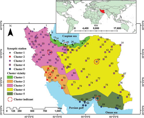
Iran is the second largest country in the Middle East (Fig. 1) with an average annual rainfall of about 230 mm, around 30% of the global average terrestrial precipitation. The mean annual precipitation in the central areas of Iran is less than 50 mm, while the corresponding value in the northern areas is typically greater than 1000 mm. It is worth noting that ¾ of the total volume of precipitation of Iran occurs over ¼ of the total area of the country. Therefore, the precipitation spatial pattern in Iran is considerably heterogeneous (Karandish and Hoekstra 2017). Raziei (2022) employed three classification methods to categorize the climate of Iran and observed that the spatial distribution of climate types corresponded to the region’s topography and proximity to water bodies. For example, all three methods identified a humid climate in the western mountainous areas of the Zagros and the northern parts of the Alborz Mountain chains. Additionally, the central-eastern and southeastern regions were consistently characterized as very arid. Consequently, we made an effort to select synoptic stations that would accurately reflect the analysis results, ensuring they were representative of the predominant climate types.

Figure 1. The study area and synoptic station clusters.

2.2 Data

A detailed description of the 41 models participating in CMIP6 whose historical simulations were used in this study is presented in Table 1. The choice of these models was based on data available at the time of the analysis. To reconcile the different spatial and temporal resolutions of the various models and observations, a resampling analysis was performed at the daily time scale for the period from 1986 to 2024.

Table 1. Information on the AR6 (The Sixth Assessment Report) climate models used in this study.

Model number	Model	Institute	Resolution (Long. × Lat.)	Reference
1	ACCESS-CM2	Australian Community Climate and Earth System Simulator (ACCESS)	1.875 × 1.25	Bi et al. (2020)
2	ACCESS-ESM1-5	Australian Community Climate and Earth System Simulator (ACCESS)	1.875 × 1.25	Ziehn et al. (2020)
3	AWI-ESM-1-1-LR	Alfred Wegener Institute (AWI)	1.88 × 1.88	Shi et al. (2020)
4	BCC-CSM2-MR	Beijing Climate Center (BCC) and China Meteorological Administration (CMA)	1.13 × 1.13	Wu et al. (2018)
5	BCC-ESM1	Beijing Climate Center (BCC) and China Meteorological Administration (CMA)	2.81 × 2.81	Zhang (2018)
6	CanESM5	Canadian Earth System Model	2.81 × 2.81	Swart et al. (2019)
7	CESM2	National Center for Atmospheric Research	1.25 × 0.94	Akinsanola et al. (2021)
8	CESM2-FV2	National Center for Atmospheric Research (NCAR)	1.9 x 2.5	Danabasoglu et al. (2019)
9	CESM2-WACCM	National Center for Atmospheric Research	1.25 × 0.94	Liao et al. (2021)
10	CMCC-CM2-HR4	Centro Euro-Mediterraneo sui Cambiamenti Climatici	1.25 × 1.875	Scoccimarro et al. (2022)
11	CMCC-CM2-SR5	Centro Euro-Mediterraneo sui Cambiamenti Climatici	1.25 × 1.875	Lovato and Peano (2020)
12	CMCC-ESM2	Centro Euro-Mediterraneo sui Cambiamenti Climatici	1.25 × 1.875	Peano et al. (2020)
13	CNRM-CM6-1	Centre National de Recherches Météorologiques (CNRM); Centre Européen de Recherches et de Formation Avancéen Calcul Scientifique	1.41 × 1.41	Voldoire et al. (2019)
14	CNRM-CM6-1-HR	Centre National de Recherches Météorologiques, Toulouse 31 057, France	0.5 × 0.5	Xin et al. (2021)
15	CNRM-ESM2-1	Centre National de Recherches Météorologiques, Toulouse 31 057, France	1.41 × 1.41	Lim Kam Sian et al. (2021)
16	EC-Earth3-AerChem	The State Meteorological Agency (AEMET) Spain	3 × 2	van Noije et al. (2021)
17	EC-Earth3-CC	The State Meteorological Agency (AEMET) Spain	3 × 2	EC-Earth (2019)
18	EC-Earth3-Veg-LR	The State Meteorological Agency (AEMET) Spain	0.7 × 0.7	Lim Kam Sian et al. (2021)
19	FGOALS-f3-L	Chinese Academy of Sciences (CAS) Flexible Global Ocean–Atmosphere–Land System	2.81 × 1.66	He et al. (2019)
20	FGOALS-g3	Chinese Academy of Sciences (CAS) Flexible Global Ocean–Atmosphere–Land System	2 × 2.25	Lim Kam Sian et al. (2021)
21	GFDL-ESM4	Geophysical Fluid Dynamics Laboratory (GFDL)	1.25 × 1.00	Krasting et al. (2018)
22	HadGEM3-GC31-LL	Met Office Hadley Centre	1.86 × 1.25	Ridley et al. (2019)
23	HadGEM3-GC31-MM	Met Office Hadley Centre	0.54 × 0.83	Xin et al. (2021)
24	IITM-ESM	Indian Institute of Tropical Meteorology Earth System Models	1.875 × 3.83	Raghavan and Panickal (2019)
25	INM-CM4-8	Institute for Numerical Mathematics, Russian Academy of Science/Russia	2 × 1.5	Lim Kam Sian et al. (2021)
26	INM-CM5-0	Institute for Numerical Mathematics, Russian Academy of Science/Russia	2 × 1.5	Lim Kam Sian et al. (2021)
27	IPSL-CM5A2-INCA	Institute Pierre-Simon Laplace (IPSL)	3.75 × 1.875	Sepulchre et al. (2020)
28	IPSL-CM6A-LR	Institute Pierre-Simon Laplace (IPSL)	2.50 × 1.26	Boucher et al. (2018)
29	KACE-1-0-G	National Institute of Meteorological Sciences/Korea Meteorological Administration, Climate Research Division, Korea	1.875 × 2.5	Byun et al. (2019)
30	KIOST-ESM	Korea Institute of Ocean Science & Technology	1.875 × 3.75	Pak et al. (2021)
31	MIROC6	Japan Agency for Marine-Earth Science and Technology, Atmosphere and Ocean Research Institute, National Institute for Environmental Studies, RIKEN Center for Computational Science	1.4 × 1.4	Lim Kam Sian et al. (2021)
32	MIROC-ES2L	Japan Agency for Marine-Earth Science and Technology, Atmosphere and Ocean Research Institute, National Institute for Environmental Studies, RIKEN Center for Computational Science	2.8 × 2.8	Lim Kam Sian et al. (2021)
33	MPI-ESM1-2-HR	Max Planck Institute for Meteorology/Germany	0.935 × 0.935	Xin et al. (2021)
34	MPI-ESM1-2-LR	Max Planck Institute for Meteorology/Germany	1.875 × 1.875	Lim Kam Sian et al. (2021)
35	MRI-ESM2-0	Meteorological Research Institute (MRI)	1.13 × 1.13	Yukimoto et al. (2019)
36	NESM3	Nanjing University of Information Science and Technology	1.875 × 1.875	Lim Kam Sian et al. (2021)
37	NorCPM1	Norwegian Climate Centre	2.5 × 3.75	Bethke et al. (2019)
38	NorESM2-MM	Norwegian Climate Centre	1.25 × 0.9374	Lim Kam Sian et al. (2021)
39	SAM0-UNICON	Seoul National University Atmosphere Model Version 0 with a Unified Convection Scheme	1.25 × 0.94	Park and Shin (2019)
40	TaiESM1	Research Center for Environmental Changes, Academia Sinica, Taiwan	1.25 × 0.9	Wang et al. (2021)
41	UKESM1-0-LL	Met Office Hadley Centre	1.88 × 1.25	Tang et al. (2023)

To compare the data simulated by GCMs with the corresponding observations, it was essential to compare them in the same spatial location. Each synoptic station was surrounded by four grid points of each GCM, and the Euclidean distance of surrounding grid points of each synoptic station was calculated. Finally, the nearest grid point to each synoptic station was assigned to it. The assigned grid point was considered the simulation of a GCM for a particular synoptic station.

To investigate climate change impacts, we used pathways 1-2.6 (SSP1-2.6) and 5-8.5 (SSP5-8.5) based on (The Sixth Assessment Report) AR6 by the Intergovernmental Panel on Climate Change (IPCC). The SSPs are the scenarios most recently developed by the IPCC to facilitate integrated analysis of vulnerabilities, adaptation, and mitigation of climate change impacts. The SSPs are based on five narratives describing alternative socio-economic developments, including sustainable (SSP1), middle of the road (SSP2), regional rivalry (SSP3), inequality (SSP4), and fossil-fueled development (SSP5). The Integrated Model to Assess the Global Environment (IMAGE) research team developed SSP1, and the Potsdam Institute for Climate Impact Research developed SSP5. A brief description of the SSPs is provided in Table 2 (O’Neill et al. 2017).

Table 2. Summary of SSP (The Shared Socio-economic Pathway) narratives.

SSP element	SSP1	SSP5
Economy and lifestyle:
Growth (per capita)	High in low-income countries (LICs), medium in high-income countries (HICs)	High
Inequality	Reduced across and within countries	Strongly reduced, especially across countries
International trade	Moderate	High, with regional specialization
Globalization	Connected markets, regional production	Strongly globalized, increasingly connected
Consumption and diet	Low growth in material consumption, low-meat diets, first in HICs	Materialism, status, consumption, tourism, mobility, meat-rich diets
Policies and institutions:
International cooperation	Effective	Effective in pursuit of development goals, more limited for environmental goals
Environmental policy	Improved management of local and global issues; tighter regulation of pollutants	Focus on local environment with obvious benefits to well-being, little concern with global problems
Policy orientation	Towards sustainable development	Towards development, free markets, human capital
Institutions	Effective at national and international levels	Increasingly effective, oriented towards fostering competitive markets
Technology:
Development	Rapid	Rapid
Transfer	Rapid	Rapid
Energy tech change	Directed away from fossil fuels, towards efficiency and renewables	Directed towards fossil fuels; alternative sources not actively pursued
Carbon intensity	Low	High
Energy intensity	Low	High
Environment and natural resources:
Fossil constraints	Preferences shift away from fossil fuels	None
Environment	Improving conditions over time	Highly engineered approaches, successful management of local issues
Land use	Strong regulations to avoid environmental tradeoffs	Medium regulations lead to slow decline in the rate of deforestation
Agriculture	Improvements in agricultural productivity; rapid diffusion of best practices	Highly managed, resource-intensive; rapid increase in productivity

2.3 Methodology

2.3.1 GCM comparison

In the present study, nine non-parametric indices describing moderate extremes with maximum return periods equal to one year were adopted according to the recommendation of (The World Meteorological Organization) WMO’s Expert Team on Climate Change Detection and Indices (ETCCDI). The indices are calculated based on daily precipitation records. Descriptions of the indices are presented in Table 3. More detail on the selected indices is provided by Zhang et al. (2011). Two statistical coefficients, percent absolute bias (PBias; Equation 1)(1) $\mathit{PBias}=\left(\frac{{\sum }_{\mathit{i}=1}^{\mathit{n}}\left|{\mathit{P}}_{\mathit{o},\mathit{i}}-{\mathit{P}}_{\mathit{h},\mathit{i}}\right|}{{\sum }_{\mathit{i}=1}^{\mathit{n}}{\mathit{P}}_{\mathit{o},\mathit{i}}}\right)\times 100$(1) and root mean square relative error (RMSRE; Equation 2(2) $\mathit{RMSRE}=\sqrt{\frac{1}{\mathit{n}}\times \sum _{\mathit{i}=1}^{\mathit{n}}{\left(\frac{{\mathit{P}}_{\mathit{o},\mathit{i}}-{\mathit{P}}_{\mathit{h},\mathit{i}}}{{\mathit{P}}_{\mathit{o},\mathit{i}}}\right)}^2}$(2) ), were used to evaluate the results related to the nine precipitation indices calculated from observed and historical GCM data:

(1) $\mathit{PBias}=\left(\frac{{\sum }_{\mathit{i}=1}^{\mathit{n}}\left|{\mathit{P}}_{\mathit{o},\mathit{i}}-{\mathit{P}}_{\mathit{h},\mathit{i}}\right|}{{\sum }_{\mathit{i}=1}^{\mathit{n}}{\mathit{P}}_{\mathit{o},\mathit{i}}}\right)\times 100$(1)

(2) $\mathit{RMSRE}=\sqrt{\frac{1}{\mathit{n}}\times \sum _{\mathit{i}=1}^{\mathit{n}}{\left(\frac{{\mathit{P}}_{\mathit{o},\mathit{i}}-{\mathit{P}}_{\mathit{h},\mathit{i}}}{{\mathit{P}}_{\mathit{o},\mathit{i}}}\right)}^2}$(2)

Table 3. List of extreme precipitation indices used in this study.

S/N	Indices	Name	Definition	Unit
1	SDII	Simple daily intensity	Let $P_{\mathit{w},\mathit{y}}$ be the daily precipitation amount on wet days, $P_w\ge 1$ mm in period $\mathit{y}$. If $\mathit{W}$ represents the number of wet days in y, then: $\mathit{SDI}{I}_y=\frac{{\sum }_{w=1}^W{P}_{\mathit{w},\mathit{y}}}{\mathit{W}}$	mm/ day
2	CDD	Consecutive dry days	Let $P_{\mathit{d},\mathit{y}}$ be the daily precipitation amount on day $\mathit{d}$ in period $\mathit{y}$. Count the largest number of consecutive days where $P_{\mathit{d},\mathit{y}}<1$ mm	day
3	CWD	Consecutive wet days	Let $P_{\mathit{d},\mathit{y}}$ be the daily precipitation amount on day $\mathit{d}$ in period $\mathit{y}$. Count the largest number of consecutive days where $P_{\mathit{d},\mathit{y}}\ge 1$ mm	day
4	PRCPTOT	Total wet-day precipitation	Let $P_{\mathit{d},\mathit{y}}$ be the daily precipitation amount on day $\mathit{d}$ in period $\mathit{y}$. If $\mathit{D}$ represents the number of days in y, then: $\mathit{PRCPTO}{T}_y=\sum _{\mathit{d}=1}^D{P}_{\mathit{d},\mathit{y}}$	mm
5	R10mm	Heavy precipitation days	Let $P_{\mathit{d},\mathit{y}}$ be the daily precipitation amount on day $\mathit{d}$ in period $\mathit{y}$. Count the number of days where $P_{\mathit{d},\mathit{y}}\ge 10$ mm	day
6	R20mm	Very heavy precipitation days	Let $P_{\mathit{dy}}$ be the daily precipitation amount on day $\mathit{d}$ in period $\mathit{y}$. Count the number of days where $P_{\mathit{d},\mathit{y}}\ge 20$ mm	day
7	RX5day	Max 5-day precipitation	Let $P_{\mathit{d},\mathit{y}}$ be the daily precipitation amount on day $\mathit{d}$ in period $\mathit{y}$. If $\mathit{D}$ represents the number of days in y, then: $\mathit{RX}5\mathit{da}{y}_y=\mathit{Max}\left\{\left(P_{\mathit{d},\mathit{y}}+P_{\mathit{d}-1,y}+P_{\mathit{d}-2,\mathit{y}}+P_{\mathit{d}-3,y}+P_{\mathit{d}-4,y}\right)\right\}$ and $\mathit{d}\in \left\{5,6,7,..,\mathit{D}\right\}$	mm
8	R95pTOT	Very wet days	Let $P_{\mathit{w},\mathit{y}}$ be the daily precipitation amount on wet days, $P_w\ge 1$ mm in period $\mathit{y},$ and let $\mathit{Pwn}95$ be the 95th percentile of precipitation on wet days in the 1986–2014 period (observation period). If W represents the number of wet days in y, then: $\mathrm{R}95\mathrm{pTO}{\mathrm{T}}_y=\sum _{\mathit{w}=1}^W{P}_{\mathit{w},\mathit{y}}$, where $P_{\mathit{w},\mathit{y}}>\mathit{Pwn}95$	mm
9	R99pTOT	Extremely wet days	Let $P_{\mathit{w},\mathit{y}}$ be the daily precipitation amount on wet days, $P_w\ge 1$ mm in period $\mathit{y},$ and let $\mathit{Pwn}99$ be the 99th percentile of precipitation on wet days in 1986–2014 period (observation period). If W represents the number of wet days in y, then: $\mathrm{R}95\mathrm{pTO}{\mathrm{T}}_y=\sum _{\mathit{w}=1}^W{P}_{\mathit{w},\mathit{y}}$, where $P_{\mathit{w},\mathit{y}}>\mathit{Pwn}99$	mm

where $P_o$ is observed precipitation, $P_h$ is the historical GCM precipitation data, and $\mathit{i}$ is the data counter.

For statistical analysis, the nine extreme precipitation indices (EPIs) (Table 3) were calculated for each station. The error measures PBias and RMSRE were computed for each station, then the average for each of the EPIs and GCMs was calculated. The total values for each measure were used to compare GCMs.

2.3.2 Downscaling and bias correction

In the current study, the Euclidean distance was used to find the closest GCM grid points to each climate station as in Equation (3)(3) $\mathbf{\Delta }{\mathit{d}}_{\mathit{a},\mathit{b}}=\sqrt{{\left(\mathit{Lo}{\mathit{n}}_{\mathit{b}}-\mathit{Lo}{\mathit{n}}_{\mathit{a}}\right)}^2+{\left(\mathit{La}{\mathit{t}}_{\mathit{b}}-\mathit{La}{\mathit{t}}_{\mathit{a}}\right)}^2}$(3) :

(3) $\mathbf{\Delta }{\mathit{d}}_{\mathit{a},\mathit{b}}=\sqrt{{\left(\mathit{Lo}{\mathit{n}}_{\mathit{b}}-\mathit{Lo}{\mathit{n}}_{\mathit{a}}\right)}^2+{\left(\mathit{La}{\mathit{t}}_{\mathit{b}}-\mathit{La}{\mathit{t}}_{\mathit{a}}\right)}^2}$(3)

where $\mathrm{\Delta }{\mathrm{d}}_{\mathrm{a},\mathrm{b}}$ is the two-dimensional spatial distance between points a and b with the specific longitude and latitude.

The period of ground-based observations used in this study is 1986 to 2015. CMIP6 historical datasets are available up to 2014. Therefore, the 29-year period from 1986 to 2014 was selected as the reference period. Statistical downscaling and bias correction were done by the quantile mapping method with the aid of the “qmap” R-package version 1-0.4 (Gudmundsson et al. 2012). The quantile mapping method is one of the most widely used methods for bias correction. The method is utilized to map the probability distribution of the simulated values based on a scenario to the probability distribution of the observed values (Gudmundsson 2012, Yang et al. 2018, Sangelantoni et al. 2019, Lee et al. 2020). Quantile mapping is implemented for the cumulative distribution functions of both the observed and simulated values over the same time period:

(4) ${\mathit{Z}}_{\mathit{i}}={\mathit{F}}_{\mathit{O}\mathit{i}}^{-1}({\mathit{F}}_{\mathit{Si}}\left({\mathit{Y}}_{\mathit{i}}\right)$(4)

where $Y_i$ is the simulation value before correction, $Z_i$ is the simulation value after calibration, $F_{\mathit{si}}$ is the cumulative distribution function of the simulated values and $F_{\mathit{oi}}$ is the cumulative distribution function of the observed values.

2.3.3 Clustering

To make the results for synoptic stations more comprehensible, we employed Delaunay triangulation clustering (DTC). In mathematics and computational geometry, the Delaunay triangle for a set of points P is a triangular plane T_s such that no point on the set of points S is inside any of the circumferential circles of $T_s$. Delaunay triangulation has been widely used in various geographic information system (GIS) applications (Liu et al. 2008, Deng et al. 2011). ArcMap software and the pseudo-F statistical method were utilized to find the optimum number of clusters (Kuswanto et al. 2021). The formula for the pseudo-F statistic is (Caliński and Harabasz 1974):

(5) $\mathit{PseudoF}=\frac{\left(\frac{{\mathit{R}}^2}{\mathit{c}-1}\right)}{\left(\frac{1-{\mathit{R}}^2}{\mathit{n}-\mathit{c}}\right)}$(5)

where $\mathit{n}$ is the number of objects, $\mathit{C}$ is the number of clusters, and $R^2$ is the coefficient of determination. For each station, the latitude, longitude, elevation, and average annual precipitation were assumed as clustering features.

2.3.4 Standardized precipitation index (SPI)

The SPI is a robust and adaptable indicator, making it a straightforward choice for drought monitoring (McKee et al. 1993). Its primary strength lies in its capacity to compare drought characteristics across varying temporal and spatial contexts and different climate types, thanks to its standardized nature (Peres et al. 2023).

A long-term precipitation time series provides the only data needed to calculate the SPI. To calculate this index, a Pearson type III distribution function (Raziei 2021) is fitted to a long-term data record of precipitation. After calculating the cumulative probability, the cumulative function is transformed into the standard norms:

(6) $\mathit{SPI}=\frac{{\mathit{P}}_{\mathit{i}}-\bar{\mathit{P}}}{\mathit{\sigma }}$(6)

where $\bar{P}$ is the average precipitation in a specific time step (e.g. monthly), $\mathit{\sigma }$ is the standard deviation, and $P_i$ is the amount of precipitation in time step i. This index can be calculated on any time scale (Hayes et al. 1999). To simplify duration–severity analysis, the time periods with negative SPI values are regarded as dry and the periods with positive SPI values are considered wet; the absolute value of the SPI thus indicates the severity of dry or wet years. The drought duration is the result of several consecutive negative SPI values.

2.3.5 Copulas and drought period calculation

If $\mathit{n}\ge 2$, then for $\mathit{G}$ as an n-dimensional distribution function with one-dimensional marginal functions $F_{x_1},\dots ,F_{x_n}$ there exists an n-copula $\mathit{C}$ (Nelsen 2006):

(7) $\mathit{G}\left({\mathit{x}}_1,\dots ,{\mathit{x}}_{\mathit{n}}\right)=\mathit{C}\left[{\mathit{F}}_{{\mathit{x}}_1}\left({\mathit{x}}_1\right),\dots ,{\mathit{F}}_{{\mathit{x}}_{\mathit{n}}}\left({\mathit{x}}_{\mathit{n}}\right)\right]$(7)

Marginal distributions can be selected independently. So, copulas have great flexibility for building a multivariate model (Srinivas et al. 2006). One of the well-known copula families is the Archimedean family. These copulas have simple forms and different dependence structures. In addition, contrary to the elliptical copulas, they have closed-form expressions which do not need to use Sklar’s theorem to be derived from multivariate distribution functions. The Archimedean bivariate copula is defined as (Nelsen 2006):

(8) $\mathit{C}\left(\mathit{u},\mathit{v}\right)={\varphi }^{-1}\left(\mathit{\varphi }\left(\mathit{u}\right),\mathit{\varphi }\left(\mathit{v}\right)\right)0<\mathit{u},\mathit{v}\le 1$(8)

where $\mathit{\varphi }$, the generator of the Archimedean copula, is a continuous, strictly decreasing function from $\left[0,1\right]$ to $\left[\left.0,\mathrm{\infty }\right)\right.$ such that $\mathit{\varphi }\left(1\right)=0$; and ${\varphi }^{\left[-1\right]}$ is the pseudo inverse of $\mathit{\varphi }$ defined in the domain $\left[\left.0,\mathrm{\infty }\right)\right.$ and range $\left[0,1\right]$:

(9) $\left\{\begin{array}{c}{\varphi }^{\left[-1\right]}\left(\mathit{x}\right)={\varphi }^{-1}\left(\mathit{x}\right)\mathit{x}\in \left[0,\mathit{\varphi }\left(0\right)\right]\\ {\varphi }^{\left[-1\right]}\left(\mathit{x}\right)=0\mathit{x}>\mathit{\varphi }\left(0\right)\end{array}\right.$(9)

Three Archimedean copulas – Clayton, Gumbel, and Frank – were applied in this study to obtain the joint distribution. Equation (11)(11) $\mathit{C}\left(\mathit{u},\mathit{v}\right)=\mathbf{max}\left({\left[{\mathit{u}}^{-\mathit{\alpha }}+{\mathit{v}}^{-\mathit{\alpha }}-1\right]}^{-1/\mathit{\alpha }},0\right)$(11) is Clayton’s copula with Equation (10)(10) $\mathit{\varphi }\left(\mathit{x}\right)=\left(\frac{1}{\mathit{\alpha }}\right)\left({\mathit{x}}^{-\mathit{\alpha }}-1\right),\mathit{\alpha }\in \left[\left.-1,\mathrm{\infty }\right)\right.$(10) as a generator (Reddy and Ganguli 2012):

(10) $\mathit{\varphi }\left(\mathit{x}\right)=\left(\frac{1}{\mathit{\alpha }}\right)\left({\mathit{x}}^{-\mathit{\alpha }}-1\right),\mathit{\alpha }\in \left[\left.-1,\mathrm{\infty }\right)\right.$(10)

(11) $\mathit{C}\left(\mathit{u},\mathit{v}\right)=\mathbf{max}\left({\left[{\mathit{u}}^{-\mathit{\alpha }}+{\mathit{v}}^{-\mathit{\alpha }}-1\right]}^{-1/\mathit{\alpha }},0\right)$(11)

Equation (13)(13) $\mathit{C}\left(\mathit{u},\mathit{v}\right)={\mathit{e}}^{\left(-{\left[{(-ln\mathit{u})}^{-\mathit{\alpha }}+{(-ln\mathit{v})}^{-\mathit{\alpha }}-1\right]}^{-1/\mathit{\alpha }}\right)}$(13) is Gumbel’s copula with Equation (12)(12) $\mathit{\varphi }\left(\mathit{x}\right)={\left(-ln\mathit{x}\right)}^{\mathit{\alpha }},\mathit{\alpha }\in \left[\left.-1,\mathrm{\infty }\right)\right.$(12) as a generator (Reddy and Ganguli 2012):

(12) $\mathit{\varphi }\left(\mathit{x}\right)={\left(-ln\mathit{x}\right)}^{\mathit{\alpha }},\mathit{\alpha }\in \left[\left.-1,\mathrm{\infty }\right)\right.$(12)

(13) $\mathit{C}\left(\mathit{u},\mathit{v}\right)={\mathit{e}}^{\left(-{\left[{(-ln\mathit{u})}^{-\mathit{\alpha }}+{(-ln\mathit{v})}^{-\mathit{\alpha }}-1\right]}^{-1/\mathit{\alpha }}\right)}$(13)

Equation (15)(15) $\mathit{C}\left(\mathit{u},\mathit{v}\right)=-\frac{1}{\mathit{\alpha }}ln\left(1+\frac{\left({\mathit{e}}^{-\mathit{\alpha u}}-1\right)-\left({\mathit{e}}^{-\mathit{\alpha v}}-1\right)}{{\mathit{e}}^{-\mathit{\alpha }}-1}\right)$(15) is Frank’s copula with Equation (14)(14) $\mathit{\varphi }\left(\mathit{x}\right)=-ln\left(\frac{{\mathit{e}}^{-\mathit{\alpha x}}-1}{{\mathit{e}}^{-\mathit{\alpha }}-1}\right),\mathit{\alpha }\ge 1$(14) as a generator (Reddy and Ganguli 2012):

(14) $\mathit{\varphi }\left(\mathit{x}\right)=-ln\left(\frac{{\mathit{e}}^{-\mathit{\alpha x}}-1}{{\mathit{e}}^{-\mathit{\alpha }}-1}\right),\mathit{\alpha }\ge 1$(14)

(15) $\mathit{C}\left(\mathit{u},\mathit{v}\right)=-\frac{1}{\mathit{\alpha }}ln\left(1+\frac{\left({\mathit{e}}^{-\mathit{\alpha u}}-1\right)-\left({\mathit{e}}^{-\mathit{\alpha v}}-1\right)}{{\mathit{e}}^{-\mathit{\alpha }}-1}\right)$(15)

where $\mathit{\alpha }$ is the parameter of the copula function that represents the dependencies between the variables $\mathit{u}$ and $\mathit{v}$. To use the copulas, there must be a significant correlation between the drought characteristics (duration and severity). Kendall, Pearson, and Spearman correlation coefficients were used to investigate the correlation between the two drought characteristics. The non-parametric method of the maximum logarithmic likelihood estimation (MLE) function was used to estimate the parameter $\mathit{\alpha }$ (Favre et al. 2004). Severity and duration are the two variables used for bivariate drought frequency analysis. Both parameters should be considered to calculate the probability of occurrence and return period to reduce uncertainty.

We used Equation (16)(16) $\begin{array}{rl}& {\mathit{P}}_{\mathit{DS}}=\mathit{P}\left(\mathit{d}\le \mathit{D}\mathbf{and}\mathit{s}\le \mathit{S}\right)={\mathit{F}}_{\mathit{DS}}\left(\mathrm{\infty },\mathrm{\infty }\right)-{\mathit{F}}_{\mathit{DS}}\left(\mathit{d},\mathrm{\infty }\right)\\ & -{\mathit{F}}_{\mathit{DS}}\left(\mathrm{\infty },\mathit{s}\right)+{\mathit{F}}_{\mathit{DS}}\left(\mathit{d},\mathit{s}\right)=1-{\mathit{F}}_{\mathit{D}}\left(\mathit{d}\right)-{\mathit{F}}_{\mathit{S}}\left(\mathit{s}\right)\\ & +\mathit{C}\left({\mathit{F}}_{\mathit{D}}\left(\mathit{d}\right),{\mathit{F}}_{\mathit{S}}\left(\mathit{s}\right)\right)\end{array}$(16) (Shiau 2006) to calculate the probability of occurrence of both severity and duration of drought when both variables are above the threshold:

(16) $\begin{array}{rl}& {\mathit{P}}_{\mathit{DS}}=\mathit{P}\left(\mathit{d}\le \mathit{D}\mathbf{and}\mathit{s}\le \mathit{S}\right)={\mathit{F}}_{\mathit{DS}}\left(\mathrm{\infty },\mathrm{\infty }\right)-{\mathit{F}}_{\mathit{DS}}\left(\mathit{d},\mathrm{\infty }\right)\\ & -{\mathit{F}}_{\mathit{DS}}\left(\mathrm{\infty },\mathit{s}\right)+{\mathit{F}}_{\mathit{DS}}\left(\mathit{d},\mathit{s}\right)=1-{\mathit{F}}_{\mathit{D}}\left(\mathit{d}\right)-{\mathit{F}}_{\mathit{S}}\left(\mathit{s}\right)\\ & +\mathit{C}\left({\mathit{F}}_{\mathit{D}}\left(\mathit{d}\right),{\mathit{F}}_{\mathit{S}}\left(\mathit{s}\right)\right)\end{array}$(16)

After calculating the joint probability using Equation (16)(16) $\begin{array}{rl}& {\mathit{P}}_{\mathit{DS}}=\mathit{P}\left(\mathit{d}\le \mathit{D}\mathbf{and}\mathit{s}\le \mathit{S}\right)={\mathit{F}}_{\mathit{DS}}\left(\mathrm{\infty },\mathrm{\infty }\right)-{\mathit{F}}_{\mathit{DS}}\left(\mathit{d},\mathrm{\infty }\right)\\ & -{\mathit{F}}_{\mathit{DS}}\left(\mathrm{\infty },\mathit{s}\right)+{\mathit{F}}_{\mathit{DS}}\left(\mathit{d},\mathit{s}\right)=1-{\mathit{F}}_{\mathit{D}}\left(\mathit{d}\right)-{\mathit{F}}_{\mathit{S}}\left(\mathit{s}\right)\\ & +\mathit{C}\left({\mathit{F}}_{\mathit{D}}\left(\mathit{d}\right),{\mathit{F}}_{\mathit{S}}\left(\mathit{s}\right)\right)\end{array}$(16) , the return period of specific duration and severity joint probability can be calculated:

(17) ${\mathit{T}}_{\mathit{DS}}=\mathit{T}\left(\mathit{D}\ge \mathit{d},\mathit{S}\ge \mathit{s}\right)=\frac{\mathit{E}\left(\mathit{L}\right)}{\mathit{P}\left(\mathit{D}\ge \mathit{d},\mathit{S}\ge \mathit{s}\right)}=\frac{\mathit{E}\left(\mathit{L}\right)}{1-{\mathit{F}}_{\mathit{D}}\left(\mathit{d}\right)-{\mathit{F}}_{\mathit{S}}\left(\mathit{s}\right)+\mathit{C}\left({\mathit{F}}_{\mathit{S}}\left(\mathit{s}\right),{\mathit{F}}_{\mathit{D}}\left(\mathit{d}\right)\right)}$(17)

where $T_{\mathit{DS}}$ is the joint return period of duration and severity, L is the time interval between the beginning of a drought and the beginning of the next drought, and E (L) is the mean of those intervals.

3 Results and discussion

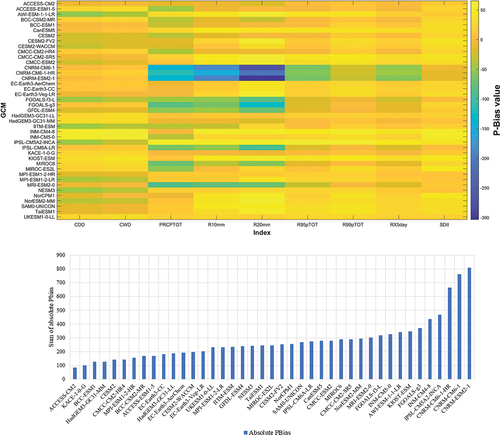
Diagrams for the two statistical measures are shown in Figs 2 and 3. The RMSRE and PBias coefficients are dimensionless, so the sum of PBias or RMSRE values for the different indices can be used to choose the models with the best performance.

Figure 2. Root mean square relative error (RMSRE) (top) and decreasing sorted sum of RMSRE (bottom) for the nine extreme precipitation indices (EPIs) for 41 GCMs.

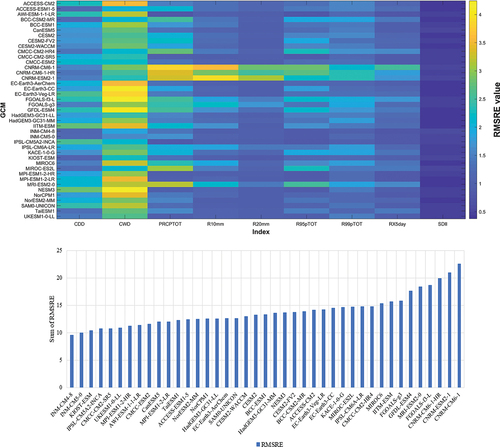
Figure 3. Percent bias (PBias) (top) and decreasing sorted sum of the absolute PBias (bottom) for the nine EPIs for 41 GCMs.

The results of the RMSRE analysis are shown in Fig. 2. The CNRM-CM6-1, CNRM-CM6-1-HR, and CNRM-ESM2-1 models substantially diverged from historical data and thus do have not sufficient accuracy for Iran. FGOALS-f3-L, MRI-ESM2-0, and GFDL-ESM4 are also unacceptable for the study area. The INM models have lower RMSRE values than other models, especially INM-CM4-8.

The PBias measure varies between −303 and 65 for the investigated GCMs. Figure 3 calculates the sum of the absolute value of the PBias for all EPIs for each GCM model. Similar to the RMSRE results, the PBias values show the CNRM models do not have acceptable accuracy. The IPSL-CM5A2-INCA and INM-CM4-8 models are also unacceptable. The best PBias result is related to the ACCESS-CM2 model.

Overall, IPSL-CM5A2-INCA, KIOST-ESM, and INM-CM4-8 had the worst PBias results but the best RMSRE results. Based on the statistical analysis, we decided to use the ACCESS-CM2 model, which has a smaller PBias than the other GCMs, and INM-CM4-8, which has a lower RMSRE than other GCMs in the study area.

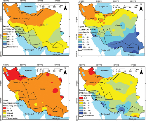
Figure 4 shows the difference between the observed and projected precipitation across Iran. The ACCESS-CM2 model shows a greater increase in precipitation than INM-CM4-8. In both GCMs, the southeast part of Iran will have a greater increase in precipitation than other regions.

Figure 4. Annual precipitation projected by GCMs (top: ACCESS-CM2, bottom: INM-CM4-8) during the future period (2023–2099) under climate change scenarios SSP1-2.6 (left) and SSP5-8.5 (right).

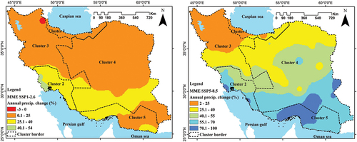
To reduce uncertainty, a multi-model ensemble (MME) of MCGCMs was created. Figure 5 shows the MME-projected precipitation variation during the future period (2023–2099). In both scenarios, the precipitation is increasing, but the precipitation change in SSP5-8.5 is about double that in SSP1-2.6. The results obtained from this research are consistent with the findings of Dezfuli et al. (2022) and the increasing pattern of precipitation from north to south. Dezfuli et al. (2022) investigated precipitation change according SSP5-8.5 based on 22 models from CMIP6. They estimated the amount of annual precipitation will increase by about 25% in the southeast of Iran but decrease by less than 10% in the northwest. Although we found a similar northwest-to-southeast increasing gradient, the future changes in precipitation estimated by our analysis were more substantial (Fig. 5).

Figure 5. MME (The Multi-Model Ensemble) projected precipitation variation during the future period (2023–2099) under climate change scenarios SSP1-2.6 (left) and SSP5-8.5 (right).

The above estimates based on CMIP6 are in sharp contrast with prior estimates of the future annual precipitation of Iran based on the results of CMIP5. Previous studies based on CMIP5 had indicated that the precipitation in Iran would be decreasing (Katiraie‐Boroujerdy et al. 2019, Zarenistanak 2019, Zamani et al. 2020, Behzadi et al. 2022). In particular, the CMIP5-based estimates of Vaghefi et al. (2019) for Iran are noteworthy. They indicated that, according to RCP4.5, humid watersheds will experience increased precipitation, while arid zones will become drier. The coastal areas of the Persian Gulf and Oman Sea will see a modest increase in precipitation (up to 50 mm/year), whereas the precipitation in other watersheds will decrease by up to 150 mm/year.

To interpret the results, the nearest synoptic station to the centre of a given cluster was chosen as the indicant of that cluster. Chalus, Ahvaz, Kabudarahang, Tabas, and Minab synoptic stations were chosen for Clusters 1 to 5, respectively. The average monthly precipitation for cluster indicants under SSP1-2.6 and SSP5-8.5 are shown in Figs 6 and 7, respectively. In Fig. 6, the average monthly precipitation of Ahvaz decreases from December to March and increases from April to November. Tabas has a similar pattern of decreasing/increasing precipitation, and the decreasing pattern is extended from October to April at Kabudarahang. According to Fig. 6, Minab will not only experience increasing spring and summer precipitation but will also have increasing precipitation in winter and late fall. Minab is the indicant of some areas that are prone to monsoon storms and rainfall in summer. The projected average monthly precipitation at Chalus is the inverse of the observed data, with intensive increasing precipitation in spring and early summer (February to July) and decreasing precipitation in fall and late summer (August to January).

Figure 6. Precipitation variation based on SSP1-2.6 and a multi-model ensemble (ACCESS-CM2 and INM-CM4-8) during the future period (2023–2099). Each plot is for a representative station of a particular cluster.

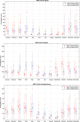
Figure 6. (Continued).

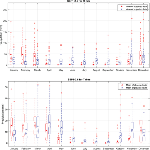
Figure 7. Precipitation variation based on SSP5-8.5 and a multi-model ensemble (ACCESS-CM2 and INM-CM4-8) during the future period (2023–2099). Each plot is for a representative station of a particular cluster.

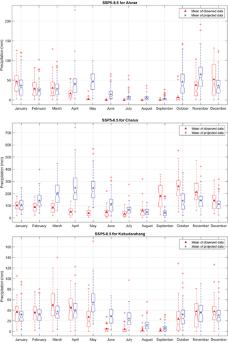
Figure 7. (Continued).

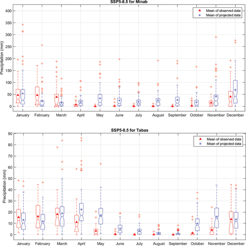
Similar to SSP1-2.6 (Fig. 6), SSP5-8.5 shows the average monthly precipitation of Ahvaz will decrease from December to March and increase from April to November (Fig. 7). This decreasing pattern is extended in Kabudarahang from late fall (December) to mid spring (April). Tabas will experience a decreasing precipitation pattern as in SSP1-2.6, except in March. The projected average monthly precipitation at Chalus again shows a pattern that is the inverse of observed data and same as SSP1-2.6. The decreasing pattern of precipitation in Minab is limited to the winter, and the pattern increases for the rest of the year.

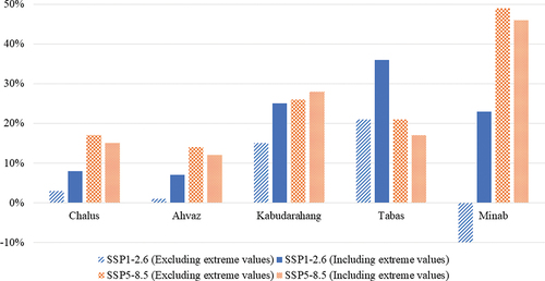
To investigate the impact of extreme values on the average annual precipitation, we calculated the averages in both conditions, i.e. including and excluding extreme values. Figure 8 demonstrates the extreme values do not sizably affect the average annual precipitation based on SSP5-8.5. However, the SSP1-2.6 simulations show major variations related to the existence of extreme values in the future. For instance, after omitting extreme values, the future average annual precipitation at Minab station will decrease by 10% in comparison with the observed average, but the average of all the future data (including extreme values) will increase by 25%. It is essential to note that a significant increase in precipitation is expected to occur in areas where frequent extreme events take place (i.e. Minab city) based on Figs 5 and 8.

Figure 8. The effect of extreme values on the observed average annual precipitation during the future period (2023–2099).

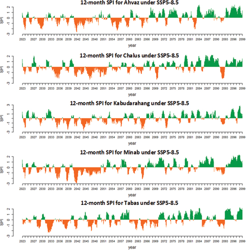
Different time scales in SPI indicate different types of droughts. Short-term SPI (less than 6 months) represents meteorological and agricultural droughts, while long-term SPI (12–48 months) demonstrates hydrological and groundwater droughts (Peres et al. 2023). Computing SPI for short time scales (3–6 months) in arid and semi-arid climates is prone to more errors due to the zero-inflated precipitation time series. So, it is recommended to use long time scales (6–12 months) to reduce the SPI calculation bias in arid and semi-arid regions (Raziei 2021). Since the dominant climate of Iran is arid and semi-arid (Vaghefi et al. 2019, Raziei 2022), the 12-month SPI was chosen as the most reliable drought index for Iran (Raziei 2021).

Recent studies propose that calculating SPI characteristics should rely on a future-inclusive period rather than historical data. This approach aims to mitigate the impact of stationary climate conditions when projecting drought index values. Additionally, it considers future adaptation and mitigation strategies (Cammalleri et al. 2022, Peres et al. 2023). In our research, we adopted a future time series as the base period for SPI calculation. By doing so, we account for nonstationary conditions and align with strategies aimed at adapting to and mitigating the effects of changing climate patterns. In summary, using future data as the reference period allows us to better address the challenges posed by climate variability and enhance the accuracy of SPI calculations.

Most droughts will happen in the early future (up to 2065) and most of the late future years (2065–2100) will be wet, based on SSP5-8.5 projections (Fig. 9). We emphasize that the increase in long-term average annual precipitation does not directly translate into an increase in water resources availability. Furthermore, we highlight that this increase alone cannot improve the situation, as other factors such as temporal shifts must also be considered.

Figure 9. The effect of extreme values on the average annual precipitation during the future period (2023–2099) for SSP5-8.5.

Droughts in terms of their severity and duration were analysed using copulas. To fit the copula functions to drought severity and duration, the parameters of the functions for the 12-month SPI were estimated (Figs 9 and 10). Copulas with the highest logarithmic maximum likelihood function were selected as the best ones (Hasebe 2013). The best-fitted copulas for each cluster are presented in Table 4. For the SSP1-2.6 outputs (severity and duration variables), the Gumbel copula is the best fitting for three clusters or stations (Chalus, Tabas, and Minab), while the Frank copula is the best fitting for the two remaining clusters or stations (Ahvaz and Kabudarahang). For the SSP5-8.5 outputs, the Frank copula is the best for three stations (Chalus, Ahvaz, and Tabas) and the Gumbel copula is the best for the two remaining stations (Kabudarahang and Minab). As such, these two copulas were identified as the best choices to fit the severity and duration output values of SSP1-2.6 and SSP5-8.5.

Figure 10. The effect of extreme values on the average annual precipitation during the future period (2023–2099) for SSP1-2.6.

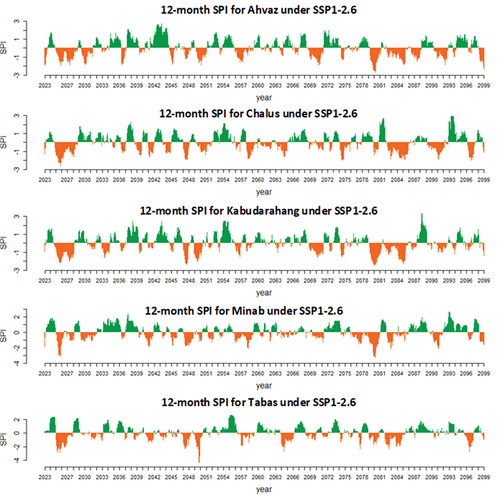
Table 4. The best-fitted distributions for copulas.

Cluster ID	Cluster indicant station	The best-fitted distributions
		SSP1-2.6	SSP5-8.5
Cluster #1	Chalus	Gumbel	Frank
Cluster #2	Ahvaz	Frank	Frank
Cluster #3	Kabudarahang	Frank	Gumbel
Cluster #4	Tabas	Gumbel	Frank
Cluster #5	Minab	Gumbel	Gumbel

Among the copulas applied in this study, Gumbel and Frank copulas were identified as the best options based on their goodness of fit to the model outputs. The Frank copula was previously introduced as a suitable option to fit the drought variables of the model outputs, by Cong and Brady (2012), Bezak et al. (2018), and Mesbahzadeh et al. (2019).

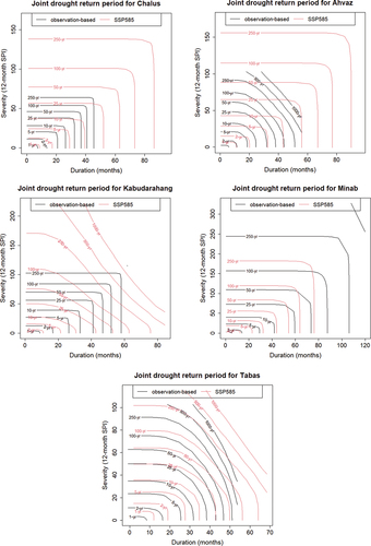
According to Fig. 11, the copulas based on the SSP1-2.6 results usually demonstrate shorter return periods than those from observation-based models in terms of both drought severity and duration. This means the same drought is more probable based on the SSP1-2.6 results than the observation-based results. The only exception is at Minab, where the return periods estimated based on the SSP1-2.6 outputs are usually greater than those calculated by the observation-based model. In addition, the similarity between the return periods estimated based on the SSP1-2.6 results and the observations is more considerable at Tabas compared to the other stations.

Figure 11. The joint drought return period due to SSP1-2.6 and multi-model ensemble (ACCESS-CM2 and INM-CM4-8).

Figure 12 shows the return periods estimated based on the SSP5-8.5 outputs and the observations. The results indicate that, for the same drought events (in terms of the severity and duration magnitudes), the copulas based on SSP5-8.5 outputs estimate shorter return periods than those estimated based on the observations. The occurrence of the same drought event is more probable based on the results of SSP5-8.5 compared to the model based on the observations. This is similar to the results provided by SSP1-2.6. However, the deviations of the return periods estimated based on SSP5-8.5 outputs from the observations-based estimates are considerably greater than those based on SSP1-2.6 outputs. Again, the results related to Minab are different from those for other stations. For the same drought events (in terms of severity and duration), the return period estimated based on the SSP5-8.5 outputs is usually longer than the return period calculated by the observation-based model. Contrary to the results related to SSP1-2.6, the return period estimates based on the SSP5-8.5 outputs at Tabas are not similar to the return periods estimated based on the observations.

Figure 12. The joint drought return period due to SSP5-8.5 and multi-model ensemble (ACCESS-CM2 and INM-CM4-8).

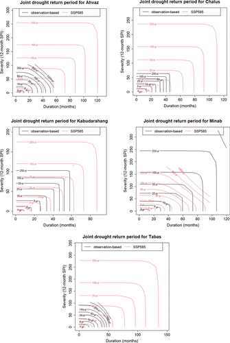
Generally, it can be concluded that in the future, drought events will intensify for the same return period, as indicated by the outputs of SSP1-2.6 and SSP5-8.5. This is consistent with the conclusion of some previous studies (e.g. Mesbahzadeh et al. 2019, Ballarin et al. 2021). While in the current study the increase is observed in both drought variables – duration and severity – Mesbahzadeh et al. (2019) and Ballarin et al. (2021) recognized the future drought intensification based on precipitation and temperature anomalies. The unique findings for the Minab station, which deviate from those for the other stations, may be attributed to its high seasonal variation in thermal and moisture characteristics, as discussed by Raziei (2022).

4 Conclusion

In this research, 41 GCMs were statistically investigated, with ACCESS-CM2 and INM-CM4-8 chosen for further study based on selection using Pbias and RMSRE statistical measures. Precipitation and drought variation in the future were investigated using a multi-GCM ensemble, which showed increasing annual precipitation but decreasing winter and fall precipitation over all of Iran except the Caspian Sea coastal area. Using SSP1-2.6, we estimated an increase by up to 40% in precipitation across the southern half of Iran (SSP5-8.5: increase by up to 100%) and an increase by up to 25% in the northern half (SSP5-8.5: increase by up to 55%). Nonetheless, only considering average annual precipitation is deceptive, as our projected precipitation indicates temporal pattern shifts in precipitation from fall and winter to spring and summer. Drought analysis showed that, for the same drought events (in terms of severity and duration), the return periods estimated based on the outputs of SSP1-2.6 and SSP5-8.5 are usually lower than estimates based on the observations, i.e. a given event is more probable based on the results provided by SSP1-2.6 and SSP5-8.5. Furthermore, SSP1-2.6 outputs seem more accurate than SSP5-8.5 outputs in terms of their deviation from the estimates based on observations.

Iran is in a water crisis, so sustainable water management is of critical importance. It is vital to consider that the increase in long-term average annual precipitation does not mean a direct increase in water resources availability, and there are more factors such as temporal shifts of precipitation to be considered. As our inter-annual projections and joint probability analysis showed, the temporal shifts in precipitation patterns or decreasing return periods of droughts will affect sustainability in the whole country in terms of impacts on crop and irrigation patterns, potable water demand, water evaporation, food security, and urban and agricultural development. The information provided herein can contribute to sustainable integrated water resources management plans. Finally, changes in temperature will impact evapotranspiration, which can affect the amount of water use. Therefore, it will be necessary to investigate temperature changes and evaporation and transpiration using this methodology in future research.

Acknowledgements

We express our thanks to the data providers.

Disclosure statement

No potential conflict of interest was reported by the author(s).

Data availability statement

All data described in the main text are available. The observed dataset of synoptic stations is available from Iran’s meteorological organization website (https://data.irimo.ir/). All climate model simulations are from CMIP6 and are publicly available, and are hosted on various servers including the Copernicus datasets (https://cds.climate.copernicus.eu/cdsapp#!/dataset/projections-cmip6?tab=form).

References

• Abbasian, M., Moghim, S., and Abrishamchi, A., 2019. Performance of the general circulation models in simulating temperature and precipitation over Iran. Theoretical and Applied Climatology, 135 (3–4), 1465–1483. doi:10.1007/s00704-018-2456-y.
   Web of Science ®Google Scholar
• Ahmed, S.M., 2020. Impacts of drought, food security policy and climate change on performance of irrigation schemes in Sub-saharan Africa: the case of Sudan. Agricultural Water Management, 232, 106064. doi:10.1016/j.agwat.2020.106064.
   Web of Science ®Google Scholar
• Akinsanola, A.A., Ongoma, V., and Kooperman, G.J., 2021. Evaluation of CMIP6 models in simulating the statistics of extreme precipitation over Eastern Africa. Atmospheric Research, 254, 105509. doi:10.1016/j.atmosres.2021.105509.
   Web of Science ®Google Scholar
• Awadh, S.M., 2023. Impact of North African sand and dust storms on the Middle East using Iraq as an example: causes, sources, and mitigation. Atmosphere, 14 (1), 180. doi:10.3390/atmos14010180.
   Web of Science ®Google Scholar
• Ballarin, A.S., et al., 2021. A copula-based drought assessment framework considering global simulation models. Journal of Hydrology: Regional Studies, 38, 100970.
   Google Scholar
• Behzadi, F., et al., 2022. Meteorological drought duration–severity and climate change impact in Iran. Theoretical and Applied Climatology, 149 (3), 1297–1315. doi:10.1007/s00704-022-04113-5.
   Web of Science ®Google Scholar
• Bethke, I., et al., 2019. NCC NorCPM1 model output prepared for CMIP6 CMIP. Norway: Earth System Grid Federation. doi:10.22033/ESGF/CMIP6.10843.
   Google Scholar
• Bezak, N., Zabret, K., and Šraj, M., 2018. Application of copula functions for rainfall interception modelling. Water, 10 (8), 995. doi:10.3390/w10080995.
   Web of Science ®Google Scholar
• Bi, D., et al., 2020. Configuration and spin-up of ACCESS-CM2, the new generation Australian community climate and earth system simulator coupled model. Journal of Southern Hemisphere Earth Systems Science, 70 (1), 225–251. doi:10.1071/ES19040.
   Web of Science ®Google Scholar
• Boucher, O., et al., 2018. Ipsl ipsl-cm6a-lr model output prepared for cmip6 cmip historical. Earth System Grid Federation. doi:10.22033/ESGF/CMIP6.5195.
   Google Scholar
• Byun, Y.-H., et al., 2019. NIMS-KMA KACE1.0-G model output prepared for CMIP6 CMIP amip. England: Earth System Grid Federation. doi:10.22033/ESGF/CMIP6.8350.
   Google Scholar
• Caliński, T. and Harabasz, J., 1974. A dendrite method for cluster analysis. Communications in Statistics-Theory and Methods, 3 (1), 1–27. doi:10.1080/03610927408827101.
   Google Scholar
• Cammalleri, C., et al., 2022. The effects of non-stationarity on SPI for operational drought monitoring in Europe. International Journal of Climatology, 42 (6), 3418–3430. doi:10.1002/joc.7424.
   Web of Science ®Google Scholar
• Clarke, L.E., 2007. Scenarios of greenhouse gas emissions and atmospheric concentrations: report. Vol. 2. Washington, DC., USA: Department of Energy, Office of Biological & Environmental Research.
   Google Scholar
• Cong, R.-G. and Brady, M., 2012. The interdependence between rainfall and temperature: copula analyses. The Scientific World Journal, 2012, 1–11. doi:10.1100/2012/405675.
   Web of Science ®Google Scholar
• Danabasoglu, G., et al., 2019. NCAR CESM2 model output prepared for CMIP6 CMIP historical. Earth System Grid Federation, Version, 20190912, 485.
   Google Scholar
• Deng, M., et al., 2011. An adaptive spatial clustering algorithm based on Delaunay triangulation. Computers, Environment and Urban Systems, 35 (4), 320–332. doi:10.1016/j.compenvurbsys.2011.02.003.
   Web of Science ®Google Scholar
• Dezfuli, A., Razavi, S., and Zaitchik, B.F., 2022. Compound effects of climate change on future transboundary water issues in the Middle East. Earth’s Future, 10 (4), e2022EF002683. doi:10.1029/2022EF002683.
   Web of Science ®Google Scholar
• (EC-Earth), E.-E. C, 2019. EC-Earth-Consortium EC-Earth3 model output prepared for CMIP6 CMIP historical. Spain: Earth System Grid Federation. doi:10.22033/ESGF/CMIP6.4700.
   Google Scholar
• Favre, A., et al., 2004. Multivariate hydrological frequency analysis using copulas. Water Resources Research, 40 (1). doi:10.1029/2003WR002456.
   Web of Science ®Google Scholar
• Fawzy, S., et al., 2020. Strategies for mitigation of climate change: a review. Environmental Chemistry Letters, 18 (6), 2069–2094. doi:10.1007/s10311-020-01059-w.
   Web of Science ®Google Scholar
• Gudmundsson, L., et al., 2012. Downscaling RCM precipitation to the station scale using statistical transformations–a comparison of methods. Hydrology and Earth System Sciences, 16 (9), 3383–3390. doi:10.5194/hess-16-3383-2012.
   Web of Science ®Google Scholar
• Gudmundsson, L., 2012. Technical note: downscaling RCM precipitation to the station scale using quantile mapping – a comparison of methods. Hydrology and Earth System Sciences Discussions, 9 (5), 6185–6201. doi:10.5194/hessd-9-6185-2012.
   Google Scholar
• Haile, G.G., et al., 2020. Projected impacts of climate change on drought patterns over East Africa. Earth’s Future, 8 (7), e2020EF001502. doi:10.1029/2020EF001502.
   Web of Science ®Google Scholar
• Hasebe, T., 2013. Copula-based maximum-likelihood estimation of sample-selection models. The Stata Journal, 13 (3), 547–573. doi:10.1177/1536867X1301300307.
   Web of Science ®Google Scholar
• Hayes, M.J., et al., 1999. Monitoring the 1996 drought using the standardized precipitation index. Bulletin of the American Meteorological Society, 80 (3), 429–438. doi:10.1175/1520-0477(1999)080<0429:MTDUTS>2.0.CO;2.
   Web of Science ®Google Scholar
• He, B., et al., 2019. CAS FGOALS-f3-L model datasets for CMIP6 historical atmospheric model Intercomparison project simulation. Advances in Atmospheric Sciences, 36 (8), 771–778. doi:10.1007/s00376-019-9027-8.
   Web of Science ®Google Scholar
• Karandish, F. and Hoekstra, A., 2017. Informing national food and water security policy through water footprint assessment: the case of Iran. Water, 9 (11), 831. doi:10.3390/w9110831.
   Web of Science ®Google Scholar
• Katiraie‐Boroujerdy, P., et al., 2019. Assessment of seven CMIP5 model precipitation extremes over Iran based on a satellite‐based climate data set. International Journal of Climatology, 39 (8), 3505–3522. doi:10.1002/joc.6035.
   Web of Science ®Google Scholar
• Krasting, J.P., et al., 2018. Noaa-gfdl gfdl-esm4 model output prepared for cmip6 cmip historical.
   Google Scholar
• Kuswanto, H., et al., 2021. Drought analysis in East Nusa Tenggara (Indonesia) using regional frequency analysis. The Scientific World Journal, 2021, 1–10. doi:10.1155/2021/6626102.
   Google Scholar
• Lee, D., et al., 2020. Future runoff analysis in the Mekong river basin under a climate change scenario using deep learning. Water (Switzerland), 12 (6), 1–19.
   Google Scholar
• Liao, E., et al., 2021. Future weakening of the ENSO ocean carbon buffer under anthropogenic forcing. Geophysical Research Letters, 48 (18), e2021GL094021. doi:10.1029/2021GL094021.
   Web of Science ®Google Scholar
• Lim Kam Sian, K.T.C., et al., 2021. Multi-decadal variability and future changes in precipitation over Southern Africa. Atmosphere, 12 (6), 742. doi:10.3390/atmos12060742.
   Web of Science ®Google Scholar
• Liu, D., Nosovskiy, G.V., and Sourina, O., 2008. Effective clustering and boundary detection algorithm based on Delaunay triangulation. Pattern Recognition Letters, 29 (9), 1261–1273. doi:10.1016/j.patrec.2008.01.028.
   Web of Science ®Google Scholar
• Lovato, T. and Peano, D., 2020. CMCC CMCC-CM2-SR5 model output prepared for CMIP6 CMIP historical. Earth System Grid Federation.
   Google Scholar
• McKee, T.B., Doesken, N.J., and Kleist, J., 1993. The relationship of drought frequency and duration to time scales. Proceedings of the 8th Conference on Applied Climatology, 17 (22), 179–183.
   Google Scholar
• Mesbahzadeh, T., et al., 2019. Joint modeling of precipitation and temperature using copula theory for current and future prediction under climate change scenarios in arid lands (case study, Kerman Province, Iran). Advances in Meteorology, 2019, 1–15. doi:10.1155/2019/6848049
   Web of Science ®Google Scholar
• Nelsen, R.B., 2006. An introduction to copulas. Portland, USA: Springer Science & Business Media.
   Google Scholar
• Noori, R., et al., 2021. Anthropogenic depletion of Iran’s aquifers. Proceedings of the National Academy of Sciences, 118 (25), e2024221118. doi:10.1073/pnas.2024221118.
   PubMed Web of Science ®Google Scholar
• O’Neill, B.C., et al., 2017. The roads ahead: narratives for shared socioeconomic pathways describing world futures in the 21st century. Global Environmental Change, 42, 169–180. doi:10.1016/j.gloenvcha.2015.01.004
   Web of Science ®Google Scholar
• Pak, G., et al., 2021. Korea institute of ocean science and technology earth system model and its simulation characteristics. Ocean Science Journal, 56 (1), 18–45. doi:10.1007/s12601-021-00001-7.
   Web of Science ®Google Scholar
• Park, S. and Shin, J., 2019. SNU SAM0-UNICON model output prepared for CMIP6 CMIP historical. Seoul, South Korea: Earth System Grid Federation.
   Google Scholar
• Peano, D., Lovato, T., and Materia, S., 2020. CMCC CMCC-ESM2 model output prepared for CMIP6 LS3MIP. France: Earth System Grid Federation. doi:10.22033/ESGF/CMIP6.13165.
   Google Scholar
• Peres, D.J., et al., 2023. A dynamic approach for assessing climate change impacts on drought: an analysis in Southern Italy. Hydrological Sciences Journal, 68.9, 1213–1228.
   Google Scholar
• Qiu, J., Shen, Z., and Xie, H., 2023. Drought impacts on hydrology and water quality under climate change. Science of the Total Environment, 858, 159854. doi:10.1016/j.scitotenv.2022.159854.
   PubMed Web of Science ®Google Scholar
• Raghavan, K. and Panickal, S., 2019. CCCR-IITM IITM-ESM model output prepared for CMIP6 CMIP piControl. India: Earth System Grid Federation.
   Google Scholar
• Raymond, C., et al., 2020. Understanding and managing connected extreme events. Nature Climate Change, 10 (7), 611–621. doi:10.1038/s41558-020-0790-4.
   Web of Science ®Google Scholar
• Raziei, T., 2021. Performance evaluation of different probability distribution functions for computing standardized precipitation index over diverse climates of Iran. International Journal of Climatology, 41 (5), 3352–3373. doi:10.1002/joc.7023.
   Web of Science ®Google Scholar
• Raziei, T., 2022. Climate of Iran according to Köppen-Geiger, Feddema, and UNEP climate classifications. Theoretical and Applied Climatology, 148 (3–4), 1395–1416. doi:10.1007/s00704-022-03992-y.
   Web of Science ®Google Scholar
• Reddy, M.J. and Ganguli, P., 2012. Bivariate flood frequency analysis of upper Godavari River flows using archimedean copulas. Water Resources Management, 26 (14), 3995–4018. doi:10.1007/s11269-012-0124-z.
   Web of Science ®Google Scholar
• Ridley, J., et al., 2019. MOHC HadGEM3-GC31-LL model output prepared for CMIP6 CMIP historical. Earth System Grid Federation. doi:10.22033/ESGF/CMIP6.6109.
   Google Scholar
• Saemian, P., et al., 2022. How much water did Iran lose over the last two decades? Journal of Hydrology: Regional Studies, 41, 101095.
   Google Scholar
• Sangelantoni, L., Russo, A., and Gennaretti, F., 2019. Impact of bias correction and downscaling through quantile mapping on simulated climate change signal: a case study over Central Italy. Theoretical and Applied Climatology, 135 (1–2), 725–740. doi:10.1007/s00704-018-2406-8.
   Web of Science ®Google Scholar
• Scoccimarro, E.,et al. 2022. Extreme events representation in CMCC-CM2 standard and high-resolution general circulation models. Geoscientific Model Development, 15, 1841–1854. doi:10.5194/gmd-15-1841-2022.
   Web of Science ®Google Scholar
• Seidler, R., et al., 2018. Progress on integrating climate change adaptation and disaster risk reduction for sustainable development pathways in South Asia: evidence from six research projects. International Journal of Disaster Risk Reduction, 31, 92–101. doi:10.1016/j.ijdrr.2018.04.023.
   Web of Science ®Google Scholar
• Sepulchre, P., et al., 2020. IPSL-CM5A2–an earth system model designed for multi-millennial climate simulations. Geoscientific Model Development, 13 (7), 3011–3053. doi:10.5194/gmd-13-3011-2020.
   Web of Science ®Google Scholar
• Shi, X., et al., 2020. Early-holocene simulations using different forcings and resolutions in AWI-ESM. The Holocene, 30 (7), 996–1015. doi:10.1177/0959683620908634.
   Web of Science ®Google Scholar
• Shiau, J.T., 2006. Fitting drought duration and severity with two-dimensional copulas. Water Resources Management, 20 (5), 795–815. doi:10.1007/s11269-005-9008-9.
   Web of Science ®Google Scholar
• Srinivas, S., Menon, D., and Meher Prasad, A., 2006. Multivariate simulation and multimodal dependence modeling of vehicle axle weights with copulas. Journal of Transportation Engineering, 132 (12), 945–955. doi:10.1061/(ASCE)0733-947X(2006)132:12(945).
   Google Scholar
• Swart, N.C., et al., 2019. The Canadian earth system model version 5 (CanESM5. 0.3). Geoscientific Model Development, 12 (11), 4823–4873. doi:10.5194/gmd-12-4823-2019.
   Web of Science ®Google Scholar
• Tang, Y.,et al., 2023. MOHC UKESM1.0-LL model output prepared for CMIP6 CMIP. World Data Center for Climate (WDCC) at DKRZ. https://www.wdc-climate.de/ui/entry?acronym=C6CMMOU0 .
   Google Scholar
• Tripathy, K.P., et al., 2023. Climate change will accelerate the high-end risk of compound drought and heatwave events. Proceedings of the National Academy of Sciences, 120 (28), e2219825120. doi:10.1073/pnas.2219825120.
   PubMed Web of Science ®Google Scholar
• Ukkola, A.M., et al., 2020. Robust future changes in meteorological drought in CMIP6 projections despite uncertainty in precipitation. Geophysical Research Letters, 47 (11), e2020GL087820. doi:10.1029/2020GL087820.
   Web of Science ®Google Scholar
• Vaghefi, S.A., et al., 2019. The future of extreme climate in Iran. Scientific Reports, 9 (1), 1–11. doi:10.1038/s41598-018-37186-2.
   PubMedGoogle Scholar
• van Noije, T., et al., 2021. EC-Earth3-AerChem: a global climate model with interactive aerosols and atmospheric chemistry participating in CMIP6. Geoscientific Model Development, 14 (9), 5637–5668. doi:10.5194/gmd-14-5637-2021.
   Web of Science ®Google Scholar
• Voldoire, A., et al., 2019. Evaluation of CMIP6 deck experiments with CNRM‐CM6‐1. Journal of Advances in Modeling Earth Systems, 11 (7), 2177–2213. doi:10.1029/2019MS001683.
   Web of Science ®Google Scholar
• Wang, Y., et al., 2021. Performance of the Taiwan earth system model in simulating climate variability compared with observations and CMIP6 model simulations. Journal of Advances in Modeling Earth Systems, 13 (7), e2020MS002353. doi:10.1029/2020MS002353.
   Web of Science ®Google Scholar
• Westley, K., et al., 2023. Climate change and coastal archaeology in the Middle East and North Africa: assessing past impacts and future threats. The Journal of Island and Coastal Archaeology, 18 (2), 251–283. doi:10.1080/15564894.2021.1955778.
   Web of Science ®Google Scholar
• Won, J., et al., 2020. Copula-based joint drought index using SPI and EDDI and its application to climate change. Science of the Total Environment, 744, 140701. doi:10.1016/j.scitotenv.2020.140701.
   PubMed Web of Science ®Google Scholar
• Wu, T., et al., 2018. BCC BCC-CSM2MR model output prepared for CMIP6 CMIP historical. Earth System Grid Federation, 10.
   Google Scholar
• Xin, X., et al., 2021. Impact of higher resolution on precipitation over China in CMIP6 HighResMIP models. Atmosphere, 12 (6), 762. doi:10.3390/atmos12060762.
   Web of Science ®Google Scholar
• Yang, X., et al., 2018. Bias correction of historical and future simulations of precipitation and temperature for China from CMIP5 models. Journal of Hydrometeorology, 19 (3), 609–623. doi:10.1175/JHM-D-17-0180.1.
   Web of Science ®Google Scholar
• Yousefi, H. and Moridi, A., 2022. Multiobjective optimization of agricultural planning considering climate change impacts: Minab reservoir upstream watershed in Iran. Journal of Irrigation and Drainage Engineering, 148 (4). doi:10.1061/(ASCE)IR.1943-4774.0001675.
   Web of Science ®Google Scholar
• Yukimoto, S., et al., 2019. MRI MRI-ESM2. 0 model output prepared for CMIP6 CMIP historical. Earth System Grid Federation.
   Google Scholar
• Zamani, Y., et al., 2020. A comparison of CMIP6 and CMIP5 projections for precipitation to observational data: the case of Northeastern Iran. Theoretical and Applied Climatology, 142 (3–4), 1613–1623. doi:10.1007/s00704-020-03406-x.
   Web of Science ®Google Scholar
• Zarenistanak, M., 2019. Historical trend analysis and future projections of precipitation from CMIP5 models in the Alborz mountain area, Iran. Meteorology and Atmospheric Physics, 131 (5), 1259–1280. doi:10.1007/s00703-018-0636-z.
   Web of Science ®Google Scholar
• Zarrin, A. and Dadashi-Roudbari, A., 2021. Projection of future extreme precipitation in Iran based on CMIP6 multi-model ensemble. Theoretical and Applied Climatology, 144 (1–2), 643–660. doi:10.1007/s00704-021-03568-2.
   Web of Science ®Google Scholar
• Zhang, J., 2018. BCC BCC-ESM1 model output prepared for CMIP6 CMIP historical. Earth System Grid Federation.
   Google Scholar
• Zhang, X., et al., 2011. Indices for monitoring changes in extremes based on daily temperature and precipitation data. Wiley Interdisciplinary Reviews: Climate Change, 2 (6), 851–870.
   Web of Science ®Google Scholar
• Ziehn, T., et al., 2020. The Australian earth system model: ACCESS-ESM1. 5. Journal of Southern Hemisphere Earth Systems Science, 70 (1), 193–214. doi:10.1071/ES19035.
   Web of Science ®Google Scholar
• Zittis, G., et al., 2022. Climate change and weather extremes in the Eastern Mediterranean and Middle East. Reviews of Geophysics, 60 (3), e2021RG000762. doi:10.1029/2021RG000762.
   Web of Science ®Google Scholar

Additional information

Funding

This research received no specific grant from any funding agency in the public, commercial, or not-for-profit sectors.