Low-flow period seasonality, trends, and climate linkages across the United States

ABSTRACT

Low-flow period properties, including timing, magnitude, and duration, influence many key processes for water resource managers and ecosystems. We computed annual low-flow period duration and timing metrics from 1951 to 2020 for 1032 conterminous United States (CONUS) streamgages and analyzed spatial patterns, trends through time, and relationships to climate. Results show northwestern and eastern CONUS streamgages had longer and more inter-annually consistent low-flow period durations, while central CONUS periods were shorter and more variable. Low-flow periods most often occurred in summer months but start and end dates occurred later in north-central and mountainous western CONUS, which have the greatest number of low flows during cold seasons. Low-flow periods are becoming longer in southeastern and northwestern CONUS but shorter in much of the rest of CONUS. Temperature was correlated with low-flow period duration in southeastern and northwestern CONUS, and precipitation was correlated with duration everywhere, but most strongly in eastern CONUS.

KEYWORDS:

• low flows
• hydrological variability
• trend analysis
• conterminous US
• streamflow

Editor S. Archfield; Associate Editor B. Bonaccorso

1 Introduction

Understanding low-flow period properties is important for meeting the needs of riverine ecosystems (Rolls et al. 2012), agriculture (Li et al. 2017), water use and supply (Naz et al. 2018), and energy production (Bartos and Chester 2015). Low flows are important components of streamflow regimes and typically occur during a specific season or seasons (Smakhtin 2001). There has been substantial interest in understanding the role of low flows in ecosystem health and diversity, such as shifts in low-flow magnitude and timing, and ecological impacts from anthropogenic and climatic factors (Carlisle et al. 2019).

In most conterminous United States (CONUS) regions, low flows primarily occur during warm seasons due to watershed moisture deficits. In some regions, mostly north-central and mountainous western CONUS, low flows often occur during cold seasons. Cold-season low flows can result from cold temperatures causing precipitation and runoff to accumulate as snow and ice rather than percolating through the shallow subsurface or contributing to short-term streamflow. Because of process differences, sites with predominantly cold-season low flows are often examined separately from those with predominantly warm-season low flows (Ehsanzadeh and Adamowski 2007, Fiala et al. 2010, Kormos et al. 2016, Laaha 2023), although evidence exists that lagged effects spanning multiple seasons or even years can influence annual low flows across seasons (Van Loon et al. 2015).

Understanding low-flow magnitudes, often quantified as the annual 7-day mean low-flow magnitude (Q7), has received much attention in the literature, principally due to the use of Q7-based metrics in management guidelines and regulations (Smakhtin 2001, US EPA 2018). Recent papers have characterized trends (Dudley et al. 2020) and seasonality (Floriancic et al. 2021) of low-flow magnitudes in CONUS and investigated the importance of precipitation, evapotranspiration, and temperature as drivers of low-flow magnitudes (Floriancic et al. 2021). Investigations considering the timing and duration of low flows often look at extreme events (Caillouet et al. 2017), such as the number of days below the Q7 10% annual exceedance probability (Pournasiri Poshtiri et al. 2019), or consider streamflow intermittency timing and duration across CONUS (Zipper et al. 2021). Some studies have considered common low-flow deficits in individual basins (Woo and Thorne 2016) or small regions. However, there has been limited investigation focused on common, or normal, low-flow period duration and timing across large regions such as CONUS. A better understanding of normal low-flow processes across the entire period of low flows, and not just the lowest inter-annual extreme, may also improve understanding of hydrological droughts, which are, by definition, timespans of abnormally low flows (Van Loon 2015). Drought metrics often focus on the duration, intensity, severity, onset (beginning), and recovery (ending) of periods of drought (Mishra and Singh 2010, Van Loon 2015). Expanding low-flow study metrics to include the duration, beginning, and ending of periods of low flows in all years of record at a site will help characterize normal conditions against which abnormal drought conditions can be compared. This study uses many of the datasets and some of the methods from a recent streamflow drought paper (Hammond et al. 2022) to evaluate low-flow period duration and timing in a similar framework to that used to evaluate drought.

While prior studies have primarily focused on the magnitude of annual or extreme low flows and their relationship to climatic variables, we further understanding of low-flow variability and its implications for hydrological drought by (1) examining national and regional patterns in normal annual low-flow period timing and duration (analogous to frost-free periods from McCabe et al. 2015); (2) computing trends in these metrics; and (3) assessing precipitation and temperature relationships to low-flow period duration, start date, and end date. Improved characterization of timing and duration provides a more complete understanding of normal, regularly occurring low-flow periods than magnitude alone.

2 Data and methods

2.1 Data

We selected 1032 USGS GAGES-II (Falcone 2011, USGS 2021) streamgages with daily streamflow data for climate years (CY = April 1 through March 31; named for the calendar year in which it ends) from 1951 through 2020. These streamgages, hereafter referred to as sites, were selected because they had streamflow data for at least 95% of days per CY, for at least 8/10 years for all decades in the time span. Climate years were chosen because they more consistently contain the entire annual low-flow period than calendar years (January through December) or water years (October through September; Carpenter and Hayes 1996, Feaster and Lee 2017). Sites where upstream reservoirs regulated more than 48 days of long-term mean daily streamflow (Wieczorek et al. 2021, Hodgkins et al. 2023) were removed to control for regulation effects on timing. We removed nested basins (>50% drainage area ratio overlap; Collins et al. 2022; see Supplementary material, Fig. S1) and non-perennial sites (>20% of days with zero flow, the threshold for low flows).

USGS National Water Information System (US Geological Survey 2021) daily streamflow data were downloaded using the R package dataRetrieval (Hirsch and DeCicco 2015, R Core Team 2021). A 7-day moving average was applied to smooth minor daily variations.

To examine relationships between annual low-flow period metrics from USGS streamgages and climate data, we obtained 5 km, spatially distributed monthly water balance model output for 1951–2020 (Wieczorek et al. 2022) forced with NOAA NClimGrid (Vose et al. 2014). Monthly grids for each variable were extracted as area-weighted watershed average time series with the exactextractr (Baston 2020) R package.

2.2 Methods

Streamflow time series were normalized by converting streamflow values to percentiles using Weibull plotting positions (Laaha et al. 2017, Hammond et al. 2022, Simeone 2022). We defined low flows as streamflows below the 20th percentile (Yevjevich 1967, McCabe et al. 2016, Austin et al. 2018). Selecting the single largest continuous low-flow period as the annual low-flow period ignored many low-flow days. Conversely, combining all CY low-flow periods captured many non-low-flow days (see Supplementary material, Fig. S2, which highlights this issue). To strike a balance between these two options and capture the maximum number of low-flow days while minimizing the inclusion of non-low-flow days, we adopted rules to conservatively eliminate low-flow periods with substantially different timing from other low-flow periods in the CY before combining the remaining periods. We eliminated low-flow periods below the 20th percentile that were shorter than 7 days or more than 45 days from another period (see Supplementary material, Fig. S3). The remaining periods were combined into the low-flow period for each CY (start date through the end date), and duration, start date, and end date metrics were computed (Fig. 1), along with 7-day low-flow magnitude. We computed each metric’s monotonic trends using Sen’s slope (Sen 1968, Helsel et al. 2020) for magnitude and the Mann-Kendall test for significance (p ≤ 0.05). We used two serial structure assumptions of time series data for the null hypotheses of the Mann-Kendall test: (1) independence, which assumes no consecutive-year data relationships, and (2) short-term persistence (AR1; Hamed and Rao 1998, Hamed 2008). Accounting for one-year lag autocorrelation (which is a measure of short-term persistence) is important when investigating low streamflows, which can be affected by a variety of processes spanning multiple years, such as groundwater contribution, making some annual low-flow period metrics correlated between neighboring years. Using a trend test that assumes independence for a time series exhibiting persistence may overestimate the statistical significance of trends (Cohn and Lins 2005, Dudley et al. 2020). Both Mann-Kendall test versions use the same test statistics, but the short-term persistence version uses an autoregressive model with a 1-year lag (AR1) to inflate the variance of the test statistic. This usually leads to lower significance (higher p values) compared to assuming independence (Dudley et al. 2020). This follows similar evaluations of trends in peak (Hodgkins et al. 2019) and low-flow period metrics (Dudley et al. 2020, Hammond and Fleming 2021). For each metric, we evaluated the suitability of assuming independence versus short-term persistence by calculating the number of sites with statistically significant lag-one autocorrelation at the 95% confidence interval (CI) (Vogel et al. 1998, Dudley et al. 2020; see Supplementary material, Fig. S4).

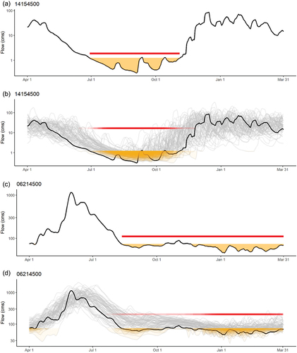
Figure 1. Low-flow period examples: (a, b) is a river (USGS 14154500) with a short low-flow period and low inter-annual variability. (c, d) is a river (USGS 06214500) with both summer and winter low-flow periods and high inter-annual variability. The x-axis is the date. The y-axis is streamflow in log-scaled cubic meters per second (cms). (a) and (c) show low-flow periods for the climate year 2004. Low flows are highlighted in yellow. The red line is the identified low-flow period. Panels (b) and (d) show all study years plotted in gray and 2004 in black. Low flows in yellow and the low-flow period in red for all years are plotted with transparency so more transparent red and yellow indicate low flows during only some years while more solid colors indicate low flows during most or all years. Additional detail can be seen in Fig. S2 (Supplementary material).

We calculated Spearman rank correlations between annual mean monthly temperature (°C) and mean monthly precipitation (mm) and annual low-flow period duration, start date, and end date to evaluate how important each climate input might be as a potential driver of low-flow periods. We considered the relative importance of the associations that precipitation and temperature each have on annual low-flow periods by calculating Spearman’s semi-partial correlations using the function spcor from the R package ppcor (Kim 2015a, 2015b). In addition, we used multiple ordinary least squares modeling with temperature, precipitation, and an interaction term as covariates to investigate the potential confounding effects of temperature and precipitation interactions on low-flow duration and timing. We also evaluated Mann-Kendall trends in annual climate values and compared them to trends in low-flow period metrics.

To identify sites with cold or warm low-flow periods, we used the mean temperature of the month with the most days of low flows for each CY. Sites with a median temperature of this month across CYs below 0°C were classified as having a predominantly cold low-flow period.

3 Results and discussion

3.1 Low-flow period properties

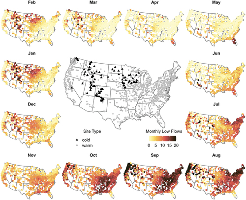
Low flows occur at most sites from August to October (Fig. 2), consistent with Q7 magnitude timing in Floriancic et al. (2021). Referring to the seven CONUS regions identified by the National Climate Adaptation Science Center (2021; see Supplementary material, Fig. S5), these sites are primarily located across eastern and northwestern CONUS. In contrast, low flows in north-central CONUS mostly occur during cold seasons in December, January, and February. Other regions, including mountainous western and southwestern CONUS, experience low flows across many months with less spatial coherence, possibly due to more variable basin properties and mixed cold-season effects.

Figure 2. The average number of low-flow days by month. Darker colors indicate more low-flow days. The center plot displays each site’s classification as having primarily cold- or warm-season low-flow periods.

Low-flow periods start earliest in southern regions, followed by eastern and coastal western CONUS. North-central and mountainous western CONUS have the latest CY start dates (Fig. 3(b)), generally agreeing with Floriancic et al. (2021). Northeastern and northwestern CONUS show the least low-flow period start date variation, while north-central CONUS shows the most variation, especially in regions with both warm and cold-season low flows. Low-flow period end dates are earliest in eastern and coastal northwestern CONUS and latest in north-central and mountainous western CONUS (Fig. 3(c)). Predominantly cold low-flow period sites have later CY start dates and end dates than warm sites but otherwise do not appear to differ substantially in overall period duration or inter-annual variability.

Figure 3. Means (panels a, b, c) and standard deviations (panels d, e, f) of low-flow period duration (days), start date, and end date (day of climate year, April 1st = 1). Histograms show the distribution of adjacent mapped metrics. Cold-season low-flow streamgages are triangular.

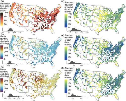
Average low-flow period durations are similar for much of CONUS (mean = 82.6 days; standard deviation = 7.61 days; Fig. 3(a); see Supplementary material, Table S1). The longest consistent low-flow periods are in eastern CONUS (except Florida); central CONUS has shorter periods but more annual variability in low-flow period duration (Fig. 3(a) and (d)). This resembles previous studies on Q7 magnitude variability and timing (Floriancic et al. 2021) and median hydrological drought durations (Hammond et al. 2022). Longer mean annual low-flow periods observed in wetter eastern CONUS as compared to drier western and central regions seems counterintuitive but could be influenced by several causes. Low-flow periods in eastern CONUS tend to be spread over longer time spans than in western CONUS since they are more commonly interspersed with convective rainfall events during their late summer period (see Supplementary material, Fig. S6(a)). Eastern CONUS has relatively few sites with multiple distinct low-flow periods which may result in one, longer single low-flow period (see Supplementary material, Fig. S6(b)). The combination of these two factors likely explains much of why eastern CONUS sites have relatively longer low-flow periods as they likely have a longer and consistent single period where low flows are possible and are more likely to briefly exceed the 20^th percentile threshold during periods when low flows are possible. Also, since we use a relative threshold, a longer low-flow period does not mean drier conditions in an absolute sense.

Eastern and northwestern CONUS have more consistent duration and timing of low-flow periods from year to year (Fig. 3(d–f)), which may result in easier identification of abnormal events, including droughts. In contrast, central CONUS has greater inter-annual variability in its low-flow period duration and timing. Western mountains, especially the Rocky Mountains, exhibit a higher degree of spatial variability in low-flow period duration and timing compared to other regions. One possible cause of this variability is that watershed properties, climate drivers (Mock 1996), and primary low-flow season (Fig. 2) are highly variable across this complex mountainous terrain.

Expanding beyond just the magnitude of low flows, especially Q7, and the timing of that magnitude provides a fuller picture of normal low-flow conditions. This fuller picture, which includes the onset, duration, magnitude, timing of the most intense low-flow magnitude, and recovery from low-flow conditions helps set a baseline of normal conditions against which periods of potential drought can be compared using common metrics of drought duration, intensity, severity, and timing.

3.2 Low-flow period trends

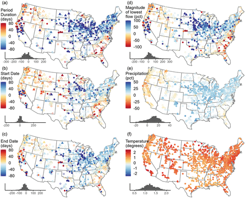
Trends in low-flow period duration vary by region. Many sites (360; 35%) show significant trends from 1951 to 2020, and most (312; 30%) indicate decreased low-flow period durations (Fig. 4). Most sites’ low-flow period duration and magnitude have lag-one autocorrelation coefficients greater than expected for an independent time series (57% and 51% at CI ≥ 95%), indicating persistence, while low-flow period start and end dates were likely to be independent (10% and 12% of sites were autocorrelated at CI ≥ 95%; see Supplementary material, Fig. S4). Sites in northeastern, midwestern, and much of south-central and western CONUS indicate trends toward shorter low-flow periods. In contrast, southeastern sites show increased low-flow period duration, as do many northwestern sites and a few in central CONUS. Spatial patterns of low-flow period start and end date trends are consistent with trend direction in low-flow period duration, although the statistical significance of trends is generally weaker. One exception is that many northern snow-influenced sites have trends toward earlier low-flow period start dates despite decreasing period durations, possibly due to earlier snowmelt (Ryberg et al. 2015). Regional patterns are similar between trends in low-flow period durations and trends in lowest streamflow magnitudes.

Figure 4. Trends in low-flow period duration, low-flow period start and end dates, low-flow magnitude, mean annual precipitation, and mean annual temperature. (a–c) are Sen-slope change over the time span in days. (d, e) are percentage Sen slope relative to the time span mean. (f) is temperature in degrees Celsius over the time span. (a, d, f) use an AR1 assumption, while (b, c, e) assume independence (see Supplementary material, Fig. S4). Red (blue) colors indicate trends toward longer (shorter) low-flow periods or drier (wetter) conditions. Cold-season low-flow streamgages are triangular. Open points represent sites with non-significant trends (p > 0.05).

Generally, spatial patterns at Hydro-Climatic Data Network (HCDN) sites, a subset of all USGS streamgages where streamflow primarily reflects prevailing meteorological conditions and have been screened to have minimal human watershed impacts (Falcone 2011, Lins 2012), and non-HCDN sites are similar across CONUS. However, density plots (see Supplementary material, Fig. S7) suggest that the non-HCDN sites tend to have slightly stronger trends toward shorter low-flow periods, with later start dates and earlier end dates than HCDN gages. In addition to potentially reflecting human impacts, this stronger trend could be influenced by the high density of non-HCDN gages relative to HCDN gages in parts of midwestern and northeastern CONUS that have strong trends toward shorter low-flow periods. Additionally, parts of southwestern CONUS, especially California, appear to have trends toward longer duration low-flow periods with earlier start dates for HCDN sites but have more mixed trends for non-HCDN sites. Overall, these results suggest that spatial patterns of trends in low flows are similar for both natural (HCDN) and modified (non-HCDN) streamgages (besides regulation). These results are consistent with results from previous studies (e.g. Ficklin et al. 2018) that reported that responses of low flows to climate change are similar for natural and modified basins.

Spatial patterns of longer low-flow periods (northwestern and southeastern CONUS) and shorter low-flow periods (northeastern and north-central CONUS) are generally consistent with trends in Q7 magnitudes (Dudley et al. 2020), 10th percentile streamflows (Rice et al. 2015), and streamflow drought duration (Hammond et al. 2022). Longer low-flow periods in northwestern and southeastern CONUS align with previous Q7 work in both regions (NW: Luce and Holden 2009, Kormos et al. 2016; SE: Stephens and Bledsoe 2020). Northwestern and southeastern regions have stronger trends toward earlier start dates than toward later end dates. We find evidence of a north–south dipole in eastern CONUS with trends toward shorter low-flow periods in the northeast and longer low-flow periods in the southeast (Kam and Sheffield 2016, Fleming et al. 2021). Sites have stronger shifts toward earlier start dates in the southeast and earlier end dates in the northeast. Results did not indicate trends toward longer low-flow periods (and aridification) in southwest CONUS. These results agree with Hammond et al. (2022), who found increasing fixed-threshold drought in southwest CONUS from 1981 to 2020, but not from 1951 to 2020. Trend beginning dates can affect the magnitude and significance of low-flow period trends (McCabe and Wolock 2002, Pournasiri Poshtiri and Pal 2016, Dethier et al. 2020, Dudley et al. 2020). We find consistent regional trend patterns across CONUS with varying beginning dates (1951–1981) through 2020 (see Supplementary material, Fig. S8), with possible exceptions of north-central and midwestern CONUS having weaker trends toward shorter low-flow periods with other trend beginning dates.

Northeastern, southeastern, and south-central regions have geographically homogeneous trends in low-flow period duration, whereas trends in western CONUS, especially California, Kansas, and Nebraska, are spatially heterogeneous. Spatial heterogeneity of trends in low-flow period durations in these regions may indicate human influences like large-scale irrigation and groundwater withdrawals (Carlisle et al. 2019, Condon and Maxwell 2019), which we see evidence of (see Supplementary material, Fig. S7).

3.3 Low-flow period drivers

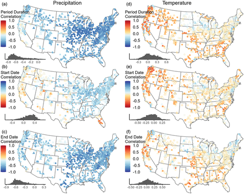
Across CONUS, low-flow period duration is negatively correlated with mean annual precipitation (more precipitation is associated with shorter low-flow periods) and generally positively correlated with mean annual temperature (Fig. 5). Precipitation is more strongly correlated with low-flow period duration and end dates in eastern CONUS than in western CONUS, as western CONUS has a higher correlation with precipitation from the previous year (see Supplementary material, Figs. S9, S10). Precipitation is positively correlated with start dates (more precipitation is associated with later start dates) in eastern CONUS but is negatively correlated with start dates in western CONUS and Florida. Temperature is most positively correlated with low-flow period duration in southeastern, south-central, and western CONUS. Temperatures are negatively correlated with start dates (higher temperature is associated with earlier start dates) and positively correlated with end dates in these regions. Sites with trends toward increased precipitation have trends toward shorter low-flow periods, later start dates, and earlier end dates (see Supplementary material, Fig. S11). In contrast, sites with the strongest increases in temperature have trends toward longer low-flow periods, earlier start dates, and later end dates.

Figure 5. Spearman correlations between mean precipitation (left) and temperature (right) and low-flow period duration (top), start date (center), and end date (bottom). Red colors indicate a positive correlation (blue is negative) between climate metrics and longer low-flow periods. Cold-season low-flow streamgages are triangular. Open points represent sites with non-significant correlations (p > 0.05).

A comparison of correlations between climate metrics (i.e. precipitation and temperature) and low-flow period duration for both HCDN and non-HCDN streamgages (see Supplementary material, Fig. S12) indicates similar regional patterns for the HCDN and non-HCDN sites as it does for trends. This similarity between HCDN and non-HCDN sites suggests that removing highly regulated sites was likely sufficient to control for omitted variable bias and multicollinearity due to anthropogenic influences at the scale of our analysis.

Both semi-partial correlations (see Supplementary material, Fig. S13) and multiple ordinary least-squares (OLS) regression models (see Supplementary material, Fig. S14) reveal that mean annual precipitation is the primary control of variability in low-flow period durations. This aligns with previous findings (e.g. McCabe and Wolock 2011) that precipitation is the primary driver of full water year runoff. Spatial patterns of correlations of precipitation with low-flow period metrics generally are minimally affected by shared variance with temperature. There are some minor exceptions in western CONUS where the semi-partial correlation of precipitation with low-flow periods is weaker after accounting for the effects of temperature, especially for the low-flow period start date (see Supplementary material, Fig. S13). Spatial patterns of slope strength between mean annual temperature and low-flow period metrics tend to be more affected by shared variance with precipitation. The addition of precipitation to multiple OLS regression models generally decreases the explanatory power of temperature on low-flow period metrics, especially in southeastern, south-central, and north-central CONUS, but surprisingly increases the explanatory power of temperature in parts of northeastern CONUS (see Supplementary material, Fig. S14). When only considering statistically significant semi-partial correlations, the explanatory power of temperature on low-flow periods remains strong in western CONUS, is weakened in eastern CONUS for low-flow period duration and start date, and is nearly eliminated in eastern CONUS for low-flow period end date (see Supplementary material, Fig. S13). These findings of the importance of temperature for low-flow periods in western CONUS match previous studies finding that temperature is a strong driver of drought in western basins such as the Colorado River Basin (e.g. Woodhouse et al. 2016). For multiple OLS models that included a precipitation–temperature interaction term, the explained percentage of variance in annual low-flow period duration is not increased. Overall, we find that precipitation has a stronger relationship with low-flow period duration and timing across CONUS than does temperature, except for western CONUS and parts of southeastern CONUS. This result holds true also when only accounting for semi-partial correlations between mean annual temperature and low-flow period metrics, demonstrating that temperature has an especially important influence on the start date of low-flow periods, while precipitation generally controls the end date of low-flow periods in these regions.

The influence of temperature on snowpack may partially explain the relatively high correlation between temperature and low-flow period duration in some snowmelt-dominated regions in western CONUS (see Supplementary material, Figs. S15, S16). Previous studies have found that warmer winter temperatures are an important factor driving long summer and shorter winter low flows (Dierauer et al. 2018) as well as early snowmelt peaks (Dudley et al. 2017), which likely result in early summer low-flow periods. Continued increases in temperatures associated with climate change may drive future decreases in baseflows (Miller et al. 2021), which may create longer low-flow period durations. Positive correlations between temperature and low-flow period duration in other parts of western and southern CONUS suggest that low-flow period duration is also affected by evapotranspiration. In contrast, low-flow period metrics in northeastern and midwestern CONUS have near-zero correlations with mean annual temperature, which agrees with Pournasiri Poshtiri et al. (2019), who found few sites with significant correlations between mean annual temperature and extreme low-flow days. Our finding that precipitation is a more important driver of low-flow period properties in eastern CONUS than temperature contrasts with Floriancic et al. (2021) who reported excess potential evapotranspiration as more important in this area. Different results on the importance of precipitation versus temperature could arise from methodological differences between studies, such as evaluating correlation versus coincidence, or could be due to differing focus on magnitude versus duration.

This work expands on previous work (e.g. Dudley et al. 2020, Floriancic et al. 2021) by examining relationships between climate drivers (i.e. temperature and precipitation) and low-flow characteristics (i.e. low-flow period start and end dates, and duration). Warming temperatures and uncertain changes in precipitation associated with climate change are expected to drive changes in annual and seasonal hydrographs that are expected to challenge water managers, especially in western CONUS (Dettinger et al. 2015). Improved understanding of the driving forces of starting and ending dates, as well as the duration, of low-flow periods is essential to inform effective water resource management. Understanding the climate drivers of low-flow periods also has ecological implications as earlier and longer low-flow periods can adversely affect ecosystems (Patterson et al. 2022). An improved understanding of spatiotemporal patterns of relationships between climate (i.e. temperature and precipitation) and normal low-flow period properties also may provide some improved context for what climate factors influence streamflow drought across CONUS.

3.4 Implications of changing low-flow periods

Changes in low-flow period timing and duration may impact water supply (Wlostowski et al. 2022), power generation (Bartos and Chester 2015), and ecosystem health (Poff and Zimmerman 2010). Shifting normal low-flow conditions may influence what are considered abnormal or drought conditions (Hammond et al. 2022, Hoylman et al. 2022). Understanding these shifts may be more complicated in regions with heterogeneous low-flow period trends or high spatial variability in low-flow period duration and timing like California, Kansas, and Nebraska.

Longer low-flow period durations in northwestern and southeastern CONUS may impact water supply for municipalities, irrigation, and power generation, especially as regional low-flow periods typically occur in summer when water demand can be highest (Griffin and Chang 1991, Gutzler and Nims 2005). Earlier regional low-flow period start dates may impact a manager’s ability to prepare for the driest parts of the year (Vano et al. 2010), while later low-flow period end dates in parts of California, Kansas, and Nebraska may impact recovery afterward. Longer low-flow period durations can have detrimental ecosystem impacts on aquatic and riparian species (Carlisle et al. 2019). Changes in low-flow period timing can disrupt the timing of species migrations and spawning, and impact juvenile survival (Carlisle et al. 2019).

Declining low-flow period durations in northeastern and midwestern CONUS may impact regional ecosystem processes such as advantages of native species (e.g. McMahon and Finlayson 2003) or certain species’ spawning characteristics (e.g. Freeman et al. 2001) that are dependent on low flows. Shorter low-flow periods could ameliorate some regional low-flow-driven water supply issues (US Geological Survey 2014), but confounding factors like changing management or increased urbanization make these water supply benefits more uncertain (Hammond and Fleming 2021).

Future temperature increases may continue to lengthen southern and western low-flow periods due to temperature-driven increases in evapotranspiration and decreases in snowpack. Some temperature influences could be offset by more uncertain changes in precipitation in southeastern CONUS (Payton et al. 2023) and increased winter precipitation but decreased summer precipitation in northwestern CONUS (Hayhoe et al. 2018). Increasing precipitation and runoff in northeastern, midwestern, and north-central CONUS may continue shortening low-flow period durations (Payton et al. 2023), although increased hydrological drought risk through the 21st century is still possible (Prudhomme et al. 2014).

3.5 Limitations

Our low-flow period identification methods have limitations and unavoidable edge cases. For instance, some sites, especially those in Florida, have low-flow periods spanning CY boundaries, resulting in potentially anomalous low-flow periods (this occurs in about 4.5% of CYs). Weak low-flow seasonality may affect the clear selection of a low-flow period at some sites. Using other methods of low-flow period identification could affect the characteristics of these events. Different cold-season selection methods such as those presented by Laaha et al. (2023) could also result in different classifications. The coarse 5 km resolution of modeled precipitation and temperature could also affect our assessment of the drivers and controls of low-flow periods, particularly in small or topographically complex basins, if finer scale processes are driving low flows.

4 Conclusions

In this study, we examined (1) patterns in annual low-flow period start date, end date, and duration across CONUS; (2) trends in low-flow period properties during 1951–2020; and (3) climate drivers of low-flow period characteristics (i.e. start dates, end dates, and duration) to improve understanding of the variability of low-flow periods and the implications for hydrological drought. Low-flow periods in CONUS are characterized by long and geographically homogeneous periods in northwestern and eastern CONUS but short and inter-annually variable periods in central CONUS. Most of CONUS has warm-season low-flow periods, concentrated in August–October. North-central and mountainous western CONUS have many low flows during cold seasons, though low-flow period duration in much of these areas has declined in recent years. In contrast, low-flow periods are becoming longer in southeastern and northwestern CONUS but shorter in other regions like midwestern and northeastern CONUS. Temperature is an important driver of low-flow period duration and timing in southeastern and western CONUS, and continued temperature increases may result in longer future low-flow periods in these regions. Precipitation is an important driver of low-flow period duration and timing across CONUS, but especially in northeastern and midwestern CONUS, where low-flow periods are minimally correlated with temperature.

Evaluating timing, duration, and magnitude metrics helps improve understanding of low-flow period properties, how they are changing, and complex interactions with their drivers, providing critical information for resource managers. This study closes a gap in how low flows and droughts have previously been studied and may also offer insight into when low-flow conditions fall below normal and become droughts.

Acknowledgements

Thank you to Christopher Konrad and two anonymous reviewers for their suggestions and edits that improved this article. Any use of trade, firm, or product names is for descriptive purposes only and does not imply endorsement by the US government. This research was funded by the US Geological Survey Water Mission Area Drought Program.

Disclosure statement

No potential conflict of interest was reported by the authors.

Data availability statement

Open Research: All data used in this study are publicly available from Simeone et al. (2023) at https://doi.org/10.5066/P9ZFKCRJ. R code used in this study is available from Simeone (2024) at https://doi.org/10.5066/P94VR71E.

Supplementary material

Supplemental data for this article can be accessed online at https://doi.org/10.1080/02626667.2024.2369639

References

- Austin, S.H., Wolock, D.M., and Nelms, D.L., 2018. Variability of hydrological droughts in the conterminous United States, 1951 through 2014. US Geological Survey Scientific Investigations Report No. 2017–5099, 16 p. doi:10.3133/sir20175099
- Bartos, M.D. and Chester, M.V., 2015. Impacts of climate change on electric power supply in the Western United States. Nature Climate Change, 5 (8), 748–752. doi:10.1038/nclimate2648.
- Baston, D., 2020. Exactextractr: fast extraction from raster datasets using polygons. R package version 0.2.0. Available from: https://CRAN.R-project.org/package=exactextractr
- Caillouet, L., et al., 2017. Ensemble reconstruction of spatio-temporal extreme low-flow events in France since 1871. Hydrology and Earth System Sciences, 21, 2923–2951. doi:10.5194/hess-21-2923-2017.
- Carlisle, D.M., et al., 2019. Flow modification in the Nation’s streams and rivers. US Geological Survey circular 1461, p. 75. doi:10.3133/cir1461.
- Carpenter, D.H. and Hayes, D.C. 1996. Low-flow characteristics of streams in Maryland and Delaware. Water-Resources Investigations Report. 94, p. 4020
- Cohn, T.A. and Lins, H.F., 2005. Nature’s style: naturally trendy. Geophysical Research Letters, 32 (23). doi:10.1029/2005GL024476.
- Collins, M.J., et al., 2022. The occurrence of large floods in the United States in the modern hydroclimate regime: seasonality, trends, and large-scale climate associations. Water Resources Research, 58, e2021WR030480. doi:10.1029/2021WR030480.
- Condon, L.E. and Maxwell, R.M., 2019. Simulating the sensitivity of evapotranspiration and streamflow to large-scale groundwater depletion. Science Advances, 5 (6), eaav4574. doi:10.1126/sciadv.aav4574.
- Dethier, E.N., et al., 2020. Spatially coherent regional changes in seasonal extreme streamflow events in the United States and Canada since 1950. Science Advances, 6 (49), eaba5939. doi:10.1126/sciadv.aba5939.
- Dettinger, M., Udall, B., and Georgakakos, A., 2015. Western water and climate change. Ecological Applications, 25 (8), 2069–2093. doi:10.1890/15-0938.1.
- Dierauer, J.R., Whitfield, P.H., and Allen, D.M., 2018. Climate controls on runoff and low flows in mountain catchments of Western North America. Water Resources Research, 54 (10), 7495–7510. doi:10.1029/2018WR023087.
- Dudley, R.W., et al., 2017. Trends in snowmelt-related streamflow timing in the conterminous United States. Journal of Hydrology, 547, 208–221. doi:10.1016/j.jhydrol.2017.01.051.
- Dudley, R.W., et al., 2020. Low streamflow trends at human-impacted and reference basins in the United States. Journal of Hydrology, 580, 124254. doi:10.1016/j.jhydrol.2019.124254.
- Ehsanzadeh, E. and Adamowski, K., 2007. Detection of trends in low flows across Canada. Canadian Water Resources Journal, 32 (4), 251–264. doi:10.4296/cwrj3204251.
- Falcone, J.A., 2011. GAGES-II: geospatial attributes of gages for evaluating streamflow (Digit. Spat. Data set). Reston, VA: US Geological Survey. doi:10.5066/P96CPHOT.
- Feaster, T.D. and Lee, K.G., 2017. Low-flow frequency and flow-duration characteristics of selected streams in Alabama through March 2014. US Geological Survey Scientific Investigations Report. p. 2017–5083, 371. doi:10.3133/sir20175083.
- Fiala, T., Ouarda, T., and Hladný, J., 2010. Evolution of low flows in the Czech Republic. Journal of Hydrology, 393 (3–4), 206–218. doi:10.1016/j.jhydrol.2010.08.018.
- Ficklin, D.L., et al., 2018. Natural and managed watersheds show similar responses to recent climate change. Proceedings of the National Academy of Sciences, 115 (34), 8553–8557. doi:10.1073/pnas.1801026115.
- Fleming, B.J., et al., 2021. Spatial and temporal patterns of low streamflow and precipitation changes in the Chesapeake Bay Watershed. JAWRA Journal of the American Water Resources Association, 57 (1), 96–108. doi:10.1111/1752-1688.12892.
- Floriancic, M.G., et al., 2021. Seasonality and drivers of low flows across Europe and the United States. Water Resources Research, 57, e2019WR026928. doi:10.1029/2019WR026928.
- Freeman, M.C., et al., 2001. Flow and habitat effects on juvenile fist abundance in natural and altered flow regimes. Ecological Applications, 11, 179–190. doi:10.1890/1051-0761(2001)011[0179:FAHEOJ]2.0.CO;2.
- Griffin, R.C. and Chang, C., 1991. Seasonality in community water demand. Western Journal of Agricultural Economics, 16 (2), 207–217. http://www.jstor.org/stable/40982746.
- Gutzler, D. S., and Nims, J. S., 2005. Interannual variability of water demand and summer climate in Albuquerque, New Mexico, Journal of Applied Meteorology. 44(12), 1777–1787. doi:10.1175/JAM2298.1.
- Hamed, K.H., 2008. Trend detection in hydrologic data: the Mann-Kendall trend test under the scaling hypothesis. Journal of Hydrology, 349, 350–363. doi:10.1016/j.jhydrol.2007.11.009.
- Hamed, K.H. and Rao, R., 1998. A modified Mann-Kendall trend test for autocorrelated data. Journal of Hydrology, 204, 182–196. doi:10.1016/S0022-1694(97)00125-X.
- Hammond, J.C., et al., 2022. Going beyond low flows: streamflow drought deficit and duration illuminate distinct spatiotemporal drought patterns and trends in the US during the last century. Water Resources Research, 58, e2022WR031930. doi:10.1029/2022WR031930.
- Hammond, J.C. and Fleming, B.J., 2021. Evaluating low flow patterns, drivers and trends in the Delaware River Basin. Journal of Hydrology, 598 (2021), 126246. doi:10.1016/j.jhydrol.2021.126246.
- Hayhoe, K., et al., 2018. Our changing climate. In: D.R. Reidmiller, et al., eds. Impacts, risks, and adaptation in the United States: fourth national climate assessment, volume II. Washington, DC, USA: US Global Change Research Program, 72–144. doi:10.7930/NCA4.2018.CH2.
- Helsel, D.R., et al., 2020, Statistical methods in water resources: US Geological Survey techniques and methods, book 4, chap. A3. p. 458. doi:10.3133/tm4a3. [ Supersedes USGS Techniques of Water-Resources Investigations, book 4, chap. A3, version 1.1.]
- Hirsch, R.M. and DeCicco, L.A., 2015. User guide to Exploration and Graphics for RivEr Trends (EGRET) and dataRetrieval: R packages for hydrologic data (version 2.0, February 2015): US Geological Survey techniques and methods book 4, chap. p. A10,93. doi:10.3133/tm4A10.
- Hodgkins, G.A., et al., 2019. Effects of climate, regulation, and urbanization on historical flood trends in the United States. Journal of Hydrology, 573, 697–709.
- Hodgkins, G.A., et al., 2023. The consequences of neglecting reservoir storage in national-scale hydrologic models: an appraisal of key streamflow statistics. Journal of the American Water Resources Association, 60 (1), 110–131.
- Hoylman, Z.H., Bocinsky, R.K., and Jencso, K.G., 2022. Drought assessment has been outpaced by climate change: empirical arguments for a paradigm shift. Nature Communications, 13, 2715. doi:10.1038/s41467-022-30316-5.
- Kam, J. and Sheffield, J., 2016. Changes in the low flow regime over the Eastern United States (1962–2011): variability, trends, and attributions. Climatic Change, 135, 639–653. doi:10.1007/s10584-015-1574-0.
- Kim, S., 2015a. ppcor: an R package for a fast calculation to semi-partial correlation coefficients. Communications for Statistical Applications and Methods, 22 (6), 665–674. doi:10.5351/CSAM.2015.22.6.665.
- Kim, S., 2015b, ppcor: partial and semi-partial (Part) correlation. R package version 1.1.
- Kormos, P.R., et al., 2016. Trends and sensitivities of low streamflow extremes to discharge timing and magnitude in Pacific Northwest mountain streams. Water Resources Research, 52, 4990–5007. doi:10.1002/2015WR018125.
- Laaha, G., et al., 2017. The European 2015 drought from a hydrological perspective. Hydrology and Earth System Sciences, 21 (6), 3001–3024. doi:10.5194/hess-21-3001-2017.
- Laaha, G., 2023. A mixed distribution approach for low-flow frequency analysis – part 1: concept, performance, and effect of seasonality. Hydrology and Earth System Sciences, 27, 689–701. doi:10.5194/hess-27-689-2023.
- Li, M., Xu, W., and Rosegrant, M.W., 2017. Irrigation, risk aversion, and water right priority under water supply uncertainty. Water Resources Research, 53, 7885–7903. doi:10.1002/2016WR019779.
- Lins, H.F., 2012. USGS hydro-climatic data network 2009 (HCDN-2009). US Geological Survey Fact. Sheet 2012–3047. doi:10.3133/fs20123047.
- Luce, C.H. and Holden, Z.A., 2009. Declining annual streamflow distributions in the Pacific Northwest United States, 1948–2006. Geophysical Research Letters, 36, L16401. doi:10.1029/2009GL039407.
- McCabe, G.J., Betancourt, J.L., and Feng, S., 2015. Variability in the start, end, and length of frost-free periods across the conterminous United States during the past century. International Journal of Climatology, 35, 4673–4680. doi:10.1002/joc.4315.
- McCabe, G.J. and Wolock, D.M., 2002. A step increase in streamflow in the conterminous United States. Geophysical Research Letters, 29 (24), 38–1. doi:10.1029/2002GL015999.
- McCabe, G.J. and Wolock, D.M., 2011. Independent effects of temperature and precipitation on modeled runoff in the conterminous United States. Water Resources Research, 47 (11). doi:10.1029/2011WR010630.
- McCabe, G.J., Wolock, D.M., and Austin, S.H., 2016. Variability of runoff‐based drought conditions in the conterminous United States. International Journal of Climatology, 37 (2), 1014–1021. doi:10.1002/joc.4756.
- McMahon, T.A. and Finlayson, B.L., 2003. Droughts and anti-droughts: the low flow hydrology of Australian rivers. Freshwater Biology, 48, 1147–1160. doi:10.1046/j.1365-2427.2003.01098.x.
- Miller, O.L., et al., 2021. How will baseflow respond to climate change in the Upper Colorado River Basin? Geophysical Research Letters, 48, e2021GL095085. doi:10.1029/2021GL095085.
- Mishra, A.K. and Singh, V.P., 2010. A review of drought concepts. Journal of Hydrology, 391 (1–2), 202–216.
- Mock, C.J., 1996. Climatic controls and spatial variations of precipitation in the western United States. Journal of Climate, 9 (5), 1111–1125. doi:10.1175/1520-0442(1996)009<1111:CCASVO>2.0.CO;2.
- National Climate Adaptation Science Center, 2021. 2021 CASC regions, US Geological Survey data release, 2021 CASC regions - sciencebase-catalog
- Naz, B.S., et al., 2018. Effects of climate change on streamflow extremes and implications for reservoir inflow in the United States. Journal of Hydrology, 556, 359–370. doi:10.1016/j.jhydrol.2017.11.027.
- Patterson, N.K., et al., 2022. Projected effects of temperature and precipitation variability change on streamflow patterns using a functional flows approach. Earth’s Future, 10, e2021EF002631. doi:10.1029/2021EF002631.
- Payton, E.A., et al., 2023. Ch. 4. Water. In: A.R. Crimmins, et al., eds. Fifth national climate assessment. Washington, DC, USA: US Global Change Research Program, 4–7. doi:10.7930/NCA5.2023.CH4.
- Poff, N.L. and Zimmerman, J.K., 2010. Ecological responses to altered flow regimes: a literature review to inform the science and management of environmental flows. Freshwater Biology, 55 (1), 194–205. doi:10.1111/j.1365-2427.2009.02272.x.
- Poshtiri, M., et al., 2019. Variability patterns of the annual frequency and timing of low streamflow days across the United States and their linkage to regional and large-scale climate. Hydrological Processes, 33 (11), 1569–1578. doi:10.1002/hyp.13422.
- Pournasiri Poshtiri, M. and Pal, I., 2016. Patterns of hydrological drought indicators in major US River basins. Climatic Change, 134 (2016), 549–563. doi:10.1007/s10584-015-1542-8.
- Prudhomme, C., et al., 2014. Hydrological droughts in the 21st century, hotspots and uncertainties from a global multimodel ensemble experiment. Proceedings of the National Academy of Sciences, 111 (9), 3262–3267. doi:10.1073/pnas.1222473110.
- R Core Team, 2021. R: A language and environment for statistical computing. R Foundation for Statistical Computing. Available from: https://www.R-project.org
- Rice, J.S., et al., 2015. Continental US streamflow trends from 1940 to 2009 and their relationships with watershed spatial characteristics. Water Resources Research, 51, 6262–6275. doi:10.1002/2014WR016367.
- Rolls, R.J., Leigh, C., and Sheldon, F., 2012. Mechanistic effects of low-flow hydrology on riverine ecosystems: ecological principles and consequences of alteration. Freshwater Science, 31 (4), 1163–1186. doi:10.1899/12-002.1.
- Ryberg, K.R., et al., 2015. Changes in seasonality and timing of peak streamflow in snow and semi-arid climates of the north-central United States, 1910–2012. Hydrological Processes, 30, 1208–1218. doi:10.1002/hyp.10693.
- Sen, P.K., 1968. Estimates of the regression coefficient based on Kendall’s tau. Journal of the American Statistical Association, 63 (324), 1379–1389. doi:10.1080/01621459.1968.10480934.
- Simeone, C.E., 2022. Streamflow drought metrics for select United States geological survey streamgages for three different time periods from 1921–2020: US Geological Survey data release. doi:10.5066/P92FAASD.
- Simeone, C.E., 2024. Low flow period seasonality trend and climate linkages across the united states software release version 1.0.0, US Geological Survey software release. doi:10.5066/P94VR71E.
- Simeone, C.E., et al., 2023. Low-flow period seasonality, trends, and climate linkages across the United States data release: US Geological Survey data release. doi:10.5066/P9ZFKCRJ.
- Smakhtin, V.U., 2001. Low flow hydrology: a review. Journal of Hydrology, 240, 147–186.U.
- Stephens, T.A. and Bledsoe, B.P., 2020. Low-flow trends at southeast United States streamflow gauges. Journal of Water Resources Planning and Management, 146 (6), 04020032. doi:10.1061/(ASCE)WR.1943-5452.0001212.
- US Environmental Protection Agency, 2018. Low flow statistics tools – a how-to handbook for NPDES permit writers: USEPA Document Number EPA-833-B-18-001. p. 39. https://www.epa.gov/sites/production/files/2018-11/documents/low_flow_stats_tools_handbook.pdf.
- US Geological Survey, 2014, Agreement of the parties to the 1954 US Supreme court decree effective June 1, 2014. Available from: http://water.usgs.gov/osw/odrm/documents/FFMP_2014_Agreement.pdf [ Accessed 5 June 2014].
- US Geological Survey, 2021, National water information system: US Geological Survey web interface. Available from: http://nwis.waterdata.usgs.gov/nwis [ Accessed 1 March 2021].
- Van Loon, A.F., 2015. Hydrological drought explained. Wiley Interdisciplinary Reviews: Water, 2 (4), 359–392. doi:10.1002/wat2.1085.
- Van Loon, A.F., et al., 2015. Hydrological drought types in cold climates: quantitative analysis of causing factors and qualitative survey of impacts. Hydrology and Earth System Sciences, 19 (4), 1993–2016. doi:10.5194/hess-19-1993-2015.
- Vano, J.A., et al., 2010. Climate change impacts on water management and irrigated agriculture in the Yakima River Basin, Washington, USA. Climatic Change, 102, 287–317. doi:10.1007/s10584-010-9856-z.
- Vogel, R.M., Tsai, Y., and Limbrunner, J.F., 1998. The regional persistence and variability of annual streamflow in the United States. Water Resources Research, 34 (12), 3445–3459. doi:10.1029/98WR02523.
- Vose, R.R.S., et al., 2014. NOAA monthly US climate gridded dataset (NClimGrid), version 1. NOAA National Centers for Environmental Information. doi:10.7289/V5SX6B56.
- Wieczorek, M.E., et al., 2022. USGS monthly water balance model inputs and outputs for the conterminous United States, 1895–2020, based on ClimGrid data. US Geological Survey data release. doi:10.5066/P9JTV1T6.
- Wieczorek, M.E., Wolock, D.M., and McCarthy, P.M., 2021. Dam impact/disturbance metrics for the conterminous United States, 1800 to 2018. US Geological Survey data release. doi:10.5066/P92S9ZX6.
- Wlostowski, A.N., et al., 2022. Dry landscapes and parched economies: a review of how drought impacts nonagricultural socioeconomic sectors in the US Intermountain West. Wiley Interdisciplinary Reviews: Water, 9 (1), e1571. doi:10.1002/wat2.1571.
- Woo, M. and Thorne, R., 2016. Summer low flow events in the Mackenzie River system. Arctic, 69 (3), 286–304. doi:10.14430/arctic4581.
- Woodhouse, C.A., et al., 2016. Increasing influence of air temperature on upper Colorado River streamflow. Geophysical Research Letters, 43, 2174–2181. doi:10.1002/2015GL067613.
- Yevjevich, V., 1967. An objective approach to definitions and investigations of continental hydrologic droughts. Hydrology Paper, 23, 18.
- Zipper, S.C., et al., 2021. Pervasive changes in stream intermittency across the United States. Environmental Research Letters, 16 (8), 084033.