Evaluating surface and subsurface fluxes in hydrological models to advance basin-scale operational water supply forecasting

ABSTRACT

Comprehensive assessments of hydrological components are crucial for enhancing operational water supply simulations. However, hydrological models are often evaluated based on their surface flow simulations, while the validation of subsurface and groundwater components tends to be overlooked or not well documented. In this study, we evaluated the outputs of two hydrological models, the Large Basin Runoff Model (LBRM) and the Weather Research and Forecasting – Hydrological modeling extension package (WRF-Hydro), for potential implementation in operational water balance forecasting in the Great Lakes region. We examined the simulated hydrological variables including surface (e.g. snow water equivalent, evapotranspiration, and streamflow), subsurface (e.g. soil moisture at different layers), and groundwater components with observed or reference data from ground-based stations and remotely sensed images. The findings of this study provide valuable insights into the capabilities and limitations of each model. These findings contribute to more informed water management strategies for the Great Lakes region.

KEYWORDS:

• validation
• intercomparison
• hydrological processes
• WRF-Hydro
• LBRM

Editor S. Archfield; Associate Editor S. M. Pingale

1 Introduction

Hydrological models employed in operational basin-scale water balance forecasting are commonly evaluated by the skill with which they simulate surface flows at daily, monthly, or even annual time steps (Fry et al. 2014, 2020, Gaborit et al. 2017). This relatively streamlined approach to skill assessment can lead to the transition of experimental models into real-world operational environments without a comprehensive understanding of how model representation of other surface (such as evapotranspiration, and snow accumulation and melt) and subsurface (e.g. soil moisture storage) processes improves or deteriorates model skill (Liu and Gupta 2007, Montanari and Koutsoyiannis 2012). In other words, hydrological land surface models adopted in operational environments can often be considered “right” (or acceptable) because they provide reasonable simulations of surface flow, but for the “wrong” reasons because they (often unknowingly) misrepresent other surface and subsurface hydrological processes (Hrachowitz et al. 2014, Garavaglia et al. 2017). Similarly, land surface models are often classified as “wrong” because they provide erroneous surface flow simulations, but without a corresponding robust analysis of what hydrological processes are represented poorly and therefore propagate into erroneous surface flow simulations (Shen and Phanikumar 2010, Archfield et al. 2015, Clark et al. 2015, Devia et al. 2015).

This common protocol for operational model development and analysis leaves several gaps in scientific knowledge, including the opportunity to identify and correct those model components leading to erroneous surface flow simulations (Kirchner 2006, Garavaglia et al. 2017). Understandably, opportunities for evaluating land surface models for operational forecasting (including, but not limited to, forecasting at basin scales) can be limited both by time constraints and by the availability of observational data to support validation at suitable spatial (including both across the land surface and at depth) and temporal scales (Biondi et al. 2012, Arsenault et al. 2018). Validation of the groundwater component of land surface models, for example, is typically ignored or considered impractical (Bingeman et al. 2006, Rajib et al. 2016, Ala-aho et al. 2017, Mai et al. 2022).

Here, we address the challenge of testing hydrological models for potential implementation in operational water balance forecasting by evaluating two models, one representing a general classification of lumped conceptual models (Croley 1983, Croley and He 2005) and another representing a state-of-the-art high-resolution physically-based model, each evaluated using a range of skill criteria across multiple model components (above and beyond surface flow alone). We apply these two models within the Laurentian Great Lakes basin, a region that holds roughly 20% of all the Earth’s fresh (unfrozen) surface water, intersects multiple sovereign nations (including the United States, Canada, and numerous First Nations), and within which there is an ongoing effort by regional federal agencies to advance seasonal and long-term water supply forecasts, and to better understand future lake water level variability (Wilcox et al. 2007, Gronewold et al. 2013, Gronewold and Rood 2019, Fry et al. 2020).

Understanding future water level variability on the Great Lakes (and, implicitly, the contribution of land runoff to the water balance) is critical from human and environmental health as well as socioeconomic perspectives; the Great Lakes shoreline is an area of significant economic development but also poses risks and challenges caused by erosion, rip currents, and water level variability that threatens safe recreational and commercial boating (EPA 2023). Importantly, Great Lakes water level variability is driven by a complex interplay between over-lake precipitation and over-lake evaporation (both of which are very high, given the vast surface areas of the Great Lakes), runoff, and groundwater discharge (Hunter et al. 2015, Fry et al. 2020, Xu et al. 2021). Multiple studies have focused on improving models of regional precipitation and evaporation (Holman et al. 2012, Charusombat et al. 2018, Gronewold et al. 2019, Hong et al. 2022); our study here focuses on developing hydrological land surface models for improving long-term Great Lakes runoff simulations and forecasts as a component of broader water level projection systems.

Multiple hydrological modeling studies have been conducted on the Laurentian Great Lakes (Croley 1983, Pietroniro et al. 2007, Kult et al. 2014, Gaborit et al. 2017) including, notably, the most recent iteration of the Great Lakes Runoff Intercomparison Project (GRIP). The GRIP study was initiated in the early 2010s to evaluate the performance of different hydrological models in simulating streamflow across the Great Lakes, with specific studies on Lake Michigan (Fry et al. 2014), Lake Ontario (Gaborit et al. 2017), Lake Erie (Mai et al. 2021) and, most recently, the entire Great Lakes basin (Mai et al. 2022). Notably, the recent Mai et al. (2022) study evaluated surface soil moisture, evapotranspiration (ET), and snow water equivalent (SWE) across 10 models with varying structures and levels of complexity. The main findings of the GRIP study are the identification of the strengths and weaknesses of various hydrological models in their ability to estimate runoff over the Great Lakes regions, which can help researchers and operational modelers better understand the differences between various hydrological models. However, despite these efforts, there are still grand challenges facing the advancement of land surface models into operational water balance modeling across the Great Lakes, many of which are comparable to challenges facing operational seasonal and long-term forecasting in other continental basins. These challenges range from appropriately representing ET rates in response to changing solar inputs (Lofgren et al. 2013, Milly and Dunne 2017), to representing areas of abundant groundwater and the correspondingly high baseflow index (that, particularly for the Great Lakes, has been historically underrepresented in regional models; Erler et al. 2019, Costa et al. 2021).

The overarching goal of this study is to enhance our understanding of how hydrological models employed for operational water balance modeling represent the diverse range of hydrological processes and to evaluate their performance against various observed or reference data. The findings of this study are expected to provide valuable insights into the potential and limitations of each model, contributing to more informed water management plans in the Great Lakes region. The two hydrological models selected for our study have been identified by Great Lakes regional federal agencies as potential components of next-generation long-term basin-scale runoff models to simulate distributions of water supply and water levels for scenarios of climate change. The first candidate, the Weather Research and Forecasting hydrological sub-routine (WRF-Hydro), was also selected as the hydrological engine for the first phase of the National Water Model (https://water.noaa.gov/about/nwm, last access: 14 September 2023) and, as part of that effort, was prepared for extension across the entire (i.e. multinational extent of the) Great Lakes basin (Mason et al. 2019). The second candidate, the Large Basin Runoff Model (LBRM) has been used for decades in both experimental and operational seasonal water supply forecasting on the Great Lakes (Gronewold et al. 2011) and was included in each of the previous phases of the long-term GRIP study (Fry et al. 2014, Gaborit et al. 2017, Mai et al. 2021, 2022). To date, however, we know of no study that has conducted a rigorous cross-comparison between LBRM and WRF-Hydro, nor any study that rigorously analyzed both the surface and subsurface hydrological components of either model (within the Great Lakes basin or elsewhere).

2 Methods

In the following sections, we provide an overview of our methodology including a summary of key features of our study area, a description of the two hydrological models selected for evaluation (along with a basis for their selection), a description of the datasets used, and a summary of our model development, testing, and assessment procedure.

2.1 Study area

We evaluated the performance of our two candidate hydrological models (described below) across selected catchments (hereafter referred to as sub-basins) within the watershed of Lake Michigan (Fig. 1). The Lake Michigan watershed is the second largest of the Great Lakes watersheds (after the Lake Superior watershed) and is the only Great Lakes watershed located entirely within the United States (EC and USEAP 2003, Fry et al. 2014). The total area of the Lake Michigan basin (including the lake itself) is 173 683 km², roughly 33% of which (57 514 km²) is the lake surface area (Hunter et al. 2015). The dominant land cover classifications across the Lake Michigan watershed are irrigated cropland and pasture (27%), deciduous broadleaf forest (24%), and wooded wetland (15%) (National Land Cover Database; Homer et al. 2015). The elevation of the basin ranges from 175 to 578 m, with an average slope of 0.33 (33%) (National Elevation Dataset; Gesch et al. 2002). The study area is covered by tills and coarse-textured sediments, which are associated with above-average groundwater infiltration (Neff et al. 2005). Over the period 2000 to 2019, the 20-year annual average rainfall and temperature were 916 mm and 7.4°C, respectively, in the Lake Michigan watershed. The annual average runoff of 362 mm is estimated using the lumped conceptual model, LBRM, which is one of the hydrological models selected in this study (details of the model description can be found in the following section). The majority of the annual rainfall (60%) falls between May and October, and 40% of the annual flow comes from spring (approximately 20% of the annual flow occurs in summer, fall, and winter).

Figure 1. Detailed map of the Lake Michigan basin including numbered sub-basins (those used in our study are shaded in grey), locations of USGS flow gages at the outlet of the sub-basins in our study, and all basin-wide readily-available GHCN SWE stations.

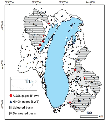
We selected the Lake Michigan basin for our study due to the abundance of observed data available for model evaluation. This basin has the highest number of observed gage stations for both streamflow and SWE (e.g. the number of stations for flow and SWE is 119 and 511, respectively), surpassing the other lake watersheds (e.g. the average number of streamflow and SWE stations for other watersheds, including Lake Superior, Erie, Huron, and Ontario, was 87 and 213, respectively; see the Supplementary material, Fig. S1). In addition, the groundwater contribution of the Lake Michigan watershed is known to be significant due to highly permeable soils and low available water capacity (Fry et al. 2014, Mei et al. 2023). Groundwater discharge comprises a large fraction of streamflow in the basin, with one estimate suggesting that groundwater contributes 66% of streamflow (details of the baseflow index map for the Lake Michigan basin can be found in the Supplementary material, Fig. S2, based on Wolock 2003). Through its contribution to streamflow, groundwater plays a crucial role in sustaining the overall water balance and hydrological processes within the Lake Michigan watershed. Understanding and accurately representing this groundwater contribution is essential for comprehensive hydrological modeling and water resource management in the Lake Michigan basin.

Notably, we chose seven sub-basins within the Lake Michigan basin for our study since the lumped conceptual model allows simulation outputs in each sub-basin considering it as a homogeneous and lumped hydrologic unit (Fig. 1). However, streamflow observations are not available at the sub-basin outlets. As streamflow gages are not located at the sub-basin outlets, we delineated the sub-basins based on their location for comparison between simulations and observations. In the Lake Michigan basin, there are many streamflow gage stations, but seven in particular were carefully chosen to represent streamflow in each sub-basin. Located closest to the sub-basin outlets, these stations ensure a robust validation process. Moreover, the overall contribution of runoff discharged into the lake inflow in the selected sub-basins is estimated to be about 43% based on the simulation results of the lumped model. Two of the selected sub-basins, 16 and 20, produce the most (11.8%) and second most (11.1%) runoff discharge among the 27 sub-basins. Consequently, the simulated flow outputs from the selected sub-basins represent a substantial part of the Lake Michigan basin’s total runoff discharge. More details about the model structure and data can be found in the following sections.

2.2 Model selection and description

In this study, we employed two operational hydrological models already calibrated by operators, the United States Army Corps of Engineers (USACE) Detroit District and National Oceanic and Atmospheric Administration (NOAA) for LBRM and WRF-Hydro, respectively. The objective of this study is to assess the performance of two important operational models representing various hydrological processes in the Great Lakes. Therefore, rather than customizing or modifying them, we keep the original configuration and parameterization of both models as they are used for actual operation of water balance and streamflow forecasting over the Great Lakes (LBRM) and the entire continental United States (WRF-Hydro) and suggest the strengths and weaknesses of the current operational set-up by examining the performance of the two models in representing various hydrological processes, which has never been explored before.

The WRF-Hydro model was originally developed by the National Center for Atmospheric Research (NCAR) as an extension of the WRF atmospheric modeling package (Gochis and Chen 2003, Gochis et al. 2020). It simulates land surface hydrology and energy states and fluxes using physics-based and conceptual approaches (Gochis et al. 2020) and has been applied across a range of global settings (Li et al. 2017, Xiang et al. 2017). The WRF-Hydro model is forced by either coupling regional atmospheric models such as the WRF model with land surface modeling or standalone land surface hydrologic modeling by employing external meteorological forcing datasets (i.e. uncoupled or offline mode). The model provides several options for land surface modeling including Noah (Ek et al. 2003) and Noah-Multiparameterization (Noah-MP; Niu et al. 2011), which is a one-dimensional column land surface model simulating the vertical fluxes of energy and moisture in land surface. These land surface processes are dynamically coupled with terrestrial hydrological processes representing surface, subsurface, channel routing, and groundwater systems.

The Large Basin Runoff Model (LBRM) is a lumped conceptual rainfall–runoff model designed to simulate sub-basin-scale runoff from the Great Lakes (Croley 1983), and was originally developed by the NOAA Great Lakes Environmental Research Laboratory (GLERL). In response to a suite of studies and workshops aimed at outlining recommended improvements to long-term hydrological forecasting models (Lofgren et al. 2011, 2013, Lofgren and Gronewold 2013, Lofgren and Rouhanaa 2016), the LBRM potential evapotranspiration (PET) formulation was recently updated by incorporating the Clausius-Clapeyron relationship (Lofgren and Rouhanaa 2016) to ensure the conservation of energy and reduce the long-term sensitivity to temperature changes. The updated LBRM model is hereafter referred to as the LBRM-CC (more details of LBRM-CC can be found in the Supplementary material, Text 1).

In this study, we employed the configuration and calibrated parameter sets of the National Water Model version 2.1 (NWMv2.1) for the WRF-Hydro simulation. Specifically, we employed the standalone Noah-MP land surface model with routing options of the steepest descent method and the Muskingum-Cunge method to represent surface overland flow routing and reach-based channel routing, respectively. For the groundwater model, we activated the exponential bucket model, which is a conceptual model used to estimate groundwater discharge based on a conceptual depth of water in the exponential bucket (detailed equations for the groundwater bucket model can be found in Gochis et al. (2020, p. 41). The same model parameter sets employed by the NWMv2.1 were adopted. The model parameters for NWMv2.1 were calibrated using the climate forcings with the Analysis of Record for Calibration (AORC; NWS-OWP 2021); Notably, AORC was specifically designed for the NWM calibration; however, AORC is not well documented in the peer-reviewed literature, and it is not a conventional source of forcing data apart from the calibration and retrospective simulation of NWM. Thus, this study employed different climate forcings for the WRF-Hydro simulation than those used to calibrate it (the details of climate forcings in this study can be found in section 2.3.1, Data for model input).

Regarding LBRM-CC, it comprises a total of 10 lumped parameters that have been successfully calibrated and used for simulating the historical basin runoff within the Great Lakes region (Fry et al. 2014, Gaborit et al. 2017). We utilized the calibrated model parameters and initial conditions for each sub-basin provided by the USACE Detroit District (via personal communication with Jonathan Waddell). The set of model parameters for LBRM-CC was calibrated for each sub-basin (Fig. 1). The calibration was performed using station-based climate forcing dataset with the Thiessen weighted interpolation, and the original data sources were obtained from the Global Historical Climatology Network – Daily (GHCN-D; Menne et al. 2012). This study employed the same climate forcings. Further details of climate forcings in this study can be found in section 2.3.1 (Data for model input).

This study employed the hydrological models calibrated exclusively for streamflow (details of model calibration can be found in the Supplementary material, Table S1). Notably, there is no official documentation of the detailed calibration and validation results specifically tailored to the Great Lakes region for both models. Therefore, our comprehensive verification in this study will provide informative insights to better understand the performance and accuracy of these models’ ability to represent the Great Lakes hydrology.

The structures of subsurface and groundwater layers differed between the two models (see the Supplementary material, Fig. S3). WRF-Hydro incorporates a 2 m soil profile with four soil layers, including depths of 10, 30, 60, and 100 cm, while LBRM-CC has a simpler soil profile with two layers, including an upper soil zone of 5 cm and a lower soil zone of 55 cm. In WRF-Hydro, subsurface lateral flow is estimated by considering exfiltration from a saturated soil column, which is then added to infiltration excess from the land surface model (Gochis et al. 2020). Moreover, WRF-Hydro employs separate surface overland flow routing and channel routing schemes to calculate surface runoff based on the land surface model (Gochis et al. 2020). In contrast, LBRM-CC represents surface and subsurface flow as fluxes from the upper and lower zone soil layers, respectively. LBRM-CC calculates all fluxes, including surface, subsurface, and groundwater fluxes, based on mass balance equations using 10 empirical parameters. Both models incorporate a highly conceptualized groundwater bucket under the soil layers. For WRF-Hydro, this groundwater bucket employed a simple exponential model controlled by three empirical parameters to calculate groundwater fluxes.

2.3 Data for model development and validation

2.3.1 Data for model input

In this study, the spatial and temporal resolution of input and output in WRF-Hydro is 1 km/hourly. Therefore, various input datasets with different spatial resolutions were regridded to 1 km resolution and then incorporated into the model (Table 1). For the meteorological forcings for WRF-Hydro, the fifth-generation European Centre for Medium-Range Weather Forecasts (ECMWF)’s atmospheric reanalysis data (ERA5; Hersbach et al. 2020) were selected to provide rainfall, air temperature, surface pressure, specific humidity, short- and longwave radiation, and wind speed (u-, v-direction) with a spatial resolution of 0.25° and an hourly temporal resolution. LBRM-CC needs daily rainfall and minimum and maximum air temperature for each sub-basin, which were derived from the interpolation of stations across the sub-basin using the Thiessen polygon-based weighting algorithm (Gronewold et al. 2011), and the station data was from the Global Historical Climatology Network – Daily (GHCN-D; Menne et al. 2012) operated by the NOAA National Centers for Environmental Information (NOAA-NCEI; https://www.glerl.noaa.gov/pubs/tech_reports/glerl-083/UpdatedFiles/daily, last access: 14 September 2023). Due to the different meteorological inputs required for the two models, we employed ERA5 and GHCN to drive WRF-Hydro and LBRM, respectively. To compare whether ERA5 and GHCN are comparable, we conducted a t-test and calculated correlation coefficients for average precipitation and temperature of 27 sub-basins in the Lake Michigan basin (see the Supplementary material, Table S2). ERA5 is a gridded hourly dataset, while GHCN is a sub-basin-wide average daily dataset. To compare the two forcings, the areal averages of ERA5 were calculated for each sub-basin and the minimum and maximum temperature of ERA5 was selected based on its hourly temperature in each day. ERA5 and GHCN were compared for monthly average precipitation and minimum and maximum temperature from 2013 to 2019 (Table S2). We found that the means of the two datasets are equal (i.e. p values in t-test greater than .05) in most cases except for the minimum temperature of the two sub-basins. In addition, the correlation coefficients are greater than 0.5 in most cases. Considering the overall trend of the two forcings is similar, we believe both forcings can be used to drive the two models. However, we acknowledge that using two different precipitation forcings may influence our study’s results. Harmonizing these inputs could be a potential aim for future research to improve robustness and accuracy.

Table 1. Summary of the data types and sources used in this study.

Data type	Item		WRF-Hydro	LBRM-CC	Spatial/temporal resolution
Model input	Spatial data	Digital elevation map	National Elevation Dataset (Gesch et al. 2002)	NA	1 arc-second (≈ 30 m)/–
		Soil	State Soil Geographic (STATSGO; Miller and White 1998)		1 km/–
		Land use	National Land Cover Database (Homer et al. 2015)		30 m/–
		River network	National Hydrography Dataset Plus V2 (McKay et al. 2012)		1 arc-second (≈ 30 m)/–
	Meteorological data		Fifth-generation European Centre for Medium-Range Weather Forecasts’ atmospheric reanalysis data (ERA5; Hersbach et al. 2020)^a	Interpolation using Thiessen polygon from Global Historical Climatology Network (GHCN; Menne et al. 2012), provided by National Oceanic and Atmospheric Administration Great Lakes Environmental Research Laboratory (NOAA-GLERL)^b	ERA5: 0.25°/hourly GHCN: Sub-basin/daily
Model output validation	Snow water equivalent (SWE)		GHCN stations		Point/daily
	Evapotranspiration (ET)		Moderate Resolution Imaging Spectroradiometer (MODIS; Running et al. 2017)^c		500 m/8-day
	Streamflow		US Geological Survey (USGS) stations		Point/daily
	Soil moisture		Global Land Evaporation Amsterdam Model (GLEAM; Martens et al. 2017)		0.25°/daily
			Soil Moisture Active Passive (SMAP; O’Neill et al. 2023)		9 km/daily
	Groundwater		Baseflow separation from streamflow observed at the USGS stations^d		Point/daily

^aHourly ERA5 variables used for WRF-Hydro: Rainfall (mm/s), air temperature (K), surface pressure (Pa), specific humidity (kg/kg), short- and longwave radiation (W/m²), and wind speed (u-, v-direction) (m/s).

^bDaily GHCN variables used for LBRM-CC: rainfall (mm), and minimum and maximum air temperature (°C). NOAA-GLERL provides meteorological data aggregated by major basins (https://www.glerl.noaa.gov/pubs/tech_reports/glerl-083/UpdatedFiles/daily/, last access: 14 September 2023).

^cMODIS ET data are updated every 8 days based on the Penman-Monteith equation using daily meteorological reanalysis data and 8-day remotely sensed vegetation property dynamics (Running et al. 2017).

^dThe baseflow index (BFI) standard method was employed to separate the baseflow using the USGS hydrologic toolbox (Barlow et al. 2015).

WRF-Hydro needs spatial information including a digital elevation map (DEM), land uses, and soils for the simulation domain (Table 1). The spatial domain employed in this study is the subset of the NWMv2.1, which used hydro-DEM data from the National Hydrography Dataset Plus version 2 (NHDPlus v2) with the National Elevation Dataset (NED) and streamflow developed by the United States Geological Survey (USGS; https://nhdplus.com/NHDPlus/, last access: 14 September 2023). The land use and soil data came from the National Land Cover Database (NLCD) produced by USGS (https://www.mrlc.gov/, last access: 14 September 2023), and from the STATSGO database (Miller and White 1998; raw data available at http://websoilsurvey.nrcs.usda.gov/, last access: 14 September 2023), respectively. More details about the spatial information can be found in Gochis et al. (2020). No spatial data was required for LBRM-CC as it is a lumped hydrological model, which considers an entire watershed as a single unit or “lump” with empirical parameters to control the various hydrological processes within the lumped unit (Croley 1983, Croley and He 2005); thus, it does not require detailed spatial data for its implementation. The sub-basin boundaries (Fig. 1) were used for the post-processing of the LBRM-CC outputs. For instance, the sub-basin boundaries were delineated based on the locations of the streamflow stations to validate simulated flow with observed flow (see section 2.4, Assessment strategy, for more details).

2.3.2 Validation data

The simulated outputs such as SWE, ET, streamflow, soil moisture storage, and groundwater flow were compared with observed (or reference) data collected from 2016 to 2019. The simulation period is notably wet in the Great Lakes region, with higher annual average rainfall (1027 mm), compared to the 20-year average from 1996 to 2015 (874 mm). This study could not evaluate the model performance in dry periods; however, wet periods can significantly impact water availability, making it vital to study how rainfall affects various hydrological components such as streamflow, soil moisture, and groundwater. Additionally, in this limited period, we could maximize our capacity to obtain various data sources for the evaluation of the various hydrological components. Future studies might consider extending the temporal scale of the simulations for a more comprehensive comparison between the two models. The SWE and streamflow data were collected at gaged stations, while ET and soil moisture storage data were obtained from the gridded remote sensed data. The SWE data were collected at GHCN-D stations within the study area (Fig. 1) and the average value of each sub-basin was calculated for the comparisons. The SWE data were obtained through the repository operated by NOAA-NCEI (https://www.ncei.noaa.gov/products/land-based-station/global-historical-climatology-network-daily, last access: 14 September 2023). The streamflow data were obtained from the USGS gage stations (https://waterdata.usgs.gov/nwis/rt, last access: 14 September 2023). The observed daily flow data were directly compared with the simulated outputs. In addition, we compared the simulated baseflow (or groundwater flux) with the reference baseflow data, which was estimated by applying the baseflow separation method to observed streamflow data. We employed the standard baseflow index method (Institute of Hydrology 1980), computed using the publicly available software program USGS Hydrologic Toolbox (Barlow et al. 2015).

Studies employed the satellite-based products to evaluate the performance of the hydrological simulation outputs (Garavaglia et al. 2017, López López et al. 2017, Srivastava et al. 2017, Bajracharya et al. 2023). In this study, we used the MOD16A2 version 6 product from Moderate Resolution Imaging Spectroradiometer (MODIS; Running et al. 2017) satellite imagery as the reference ET dataset. MODIS ET is an 8-day composite dataset with a spatial resolution of 500 m, which was used to evaluate the LBRM-CC and WRF-Hydro ET simulations. MODIS ET products utilize a combination of satellite observations (e.g. daily meteorological reanalysis data and 8-day vegetation property dynamics) and modeling techniques (Penman-Monteith equation; Monteith 1965) to estimate ET (Running et al. 2017). For the reference soil water storage dataset, we used two satellite-based products, Global Land Evaporation Amsterdam Model (GLEAM) version 3.5b (Martens et al. 2017) and Soil Moisture Active Passive (SMAP) enhanced L3 surface soil moisture version 6 (O’Neill et al. 2023). GLEAM and SMAP measure surface soil moisture from satellites, whereas the root zone soil moisture is derived from land surface modeling and data assimilation (Martens et al. 2017, O’Neill et al. 2023). For both products, surface soil depth is 5 cm, while root zone depth varies depending on land cover type (e.g. 5 cm to maximum rooting depth for vegetation) (Fig. S3). We evaluated surface soil moisture simulations using both satellite-based products from GLEAM and SMAP. We evaluated the other layers’ soil moisture simulations using the root zone soil moisture output from GLEAM, since both GLEAM and SMAP provide land surface modeling output for the root zone layer, so we just used one product. The surface soil moisture of GLEAM and SMAP was compared with the simulated soil moisture at the first layer of each model (i.e. the soil layer 1 of WRF-Hydro’s layer and the upper soil zone of LBRM-CC in Fig. S3), and soil moisture in the root zone of GLEAM was compared with the simulated soil moisture in the rest of the model (i.e. the soil layers 2, 3, and 4 of WRF-Hydro and the lower soil zone of LBRM-CC in Fig. S3).

2.4 Assessment strategy

The simulation period for this study spans 4 years, from 2016 to 2019, with a spin-up period of 3 years. The model performance was evaluated at the sub-basin scale. Thus, an area average value was calculated for each sub-basin. Comparisons were performed with a coarser temporal resolution to match temporal resolution between datasets. The assessment of various hydrological components was divided into three parts: surface (SWE, ET, and streamflow), subsurface (soil water storage in each layer), and groundwater components. For the surface components, we calculated three types of goodness-of-fit statistics including daily and monthly Nash-Sutcliffe efficiency (NSE; Nash and Sutcliffe 1970) and the absolute percentage bias (PBIAS) for the seven selected sub-basins in the Lake Michigan basin. NSE measures the absolute difference between the simulated and observed values normalized by the observation’s variance, ranging from −∞ to 1 with an optimal value of 1. We also employed PBIAS, which measures the relative errors of simulated values with an optimal value of 0%. These statistics were then visualized using radar charts to identify spatial consistencies or trends in the model performance. Additionally, we conducted a qualitative comparison by plotting daily and monthly time-series data, as well as monthly biases, for one sub-basin as an example (the time-series plots for all other sub-basins are included in the Supplementary material, Figs. S8 to S14). We focused on monthly biases rather than daily biases because the study aimed to address long-term operational water supply modeling, and monthly scale biases are more relevant for this purpose. For the subsurface and groundwater components, we used only the PBIAS statistic for evaluation due to the challenges in directly comparing the reference and simulated data. For instance, all the soil moisture data sources (GLEAM, WRF-Hydro, and LBRM-CC) had different definitions of soil layers (Fig. S3), and the reference data for groundwater components were estimated using the baseflow separation method (or linear regression). Thus, a qualitative comparison was deemed more helpful for these variables to understand the overall trends and behavior of the reference and simulated data.

For streamflow and baseflow, we directly compared the simulated and observed data at each streamflow gage station. In the case of WRF-Hydro, streamflow outputs were available at every reach, allowing for straightforward comparison with the observed data. For LBRM-CC, which represents total runoff volume at the sub-basin outlet, we delineated the sub-basins based on the locations of the streamflow gage stations (Fig. 1) and applied areal ratios to the simulated flow for direct comparisons with the observed flow based on the assumption of uniform flow within the sub-basin, implying that the flow simulated by LBRM at a specific gage is proportional to the upstream area of that sub-basins relative to the total area of the sub-basin. For other variables such as SWE, ET, and soil moisture, the median of observed stations (e.g. GHCN stations for SWE as seen in Fig. 1) or reference remote sensing products (e.g. MODIS for ET and GLEAM for soil moisture content) was calculated within each sub-basin area as a representative value for each sub-basin. Similarly, WRF-Hydro provides gridded land surface modeling outputs with 1 km resolution; thus, the median values within each sub-basin area were used to calculate goodness-of-fit measures compared to the observed or reference datasets. LBRM-CC provides simulated outputs for each sub-basin, which were directly used to calculate goodness-of-fit statistics. The soil water storage dataset in GLEAM and WRF-Hydro represents volumetric soil water content, which is the fraction of the total volume of water to the total volume of soil, while those in LBRM-CC are soil water depth. To ensure a consistent comparison, we converted the soil water depth in LBRM-CC to volumetric soil water content (e.g. soil water depth/total soil depth in each layer) and then compared it with the reference data.

3 Results

3.1 Surface components: SWE, ET, and streamflow

The results of the study indicate that LBRM-CC performed better than WRF-Hydro in simulating SWE and streamflow, while WRF-Hydro exhibited better performance in simulating ET (Fig. 2). In the case of SWE, LBRM-CC showed higher NSE in most sub-basins, except for sub-basins 5 and 16. However, both models struggled to accurately simulate daily SWE, showing a wide range of NSE values (e.g. −0.94 to 0.58 for WRF-Hydro and −1.06 to 0.70 for LBRM-CC) in the selected sub-basins (Fig. 2). The performance of simulating daily SWE varied depending on the location, which can be attributed to the models’ inability to accurately simulate the daily dynamics of SWE as well as the quality of the observed SWE datasets due to the discrepancy in station density. There were substantial variations in the number of SWE monitoring stations among sub-basins, ranging from 2 in sub-basin 8 to 55 in sub-basin 20 (Fig. 1), which may have impacted the quality of the observed SWE data and influenced the accuracy statistics at the daily scale. Monthly averaging helps to smooth out the variability and noise that may be present in daily data and capture the cumulative effects of temperature, solar radiation, and snowpack characteristics. The accuracy statistics for monthly NSE showed improved performance compared to the daily scale. For example, the range of monthly NSE values in the selected sub-basins was 0.32 to 0.74 for WRF-Hydro and 0.30 to 0.91 for LBRM-CC. The average PBIAS of SWE for all sub-basins was around 30% for both models. Overall, both models are capable of capturing the general trends in observed SWE, including timing and average amount (Fig. 3 and the time-series comparison for other sub-basins can be found in the Supplementary material, Figs. S8 to 14).

Figure 2. Evaluation of simulated surface components from WRF-Hydro and LBRM-CC across all Lake Michigan sub-basins in our study (labeled only in subplot “a” for clarity) including SWE (top row), ET (middle row), and streamflow (bottom row) based on NSE calculated at daily (left column) and monthly (middle column) time steps, and on PBIAS (right column).

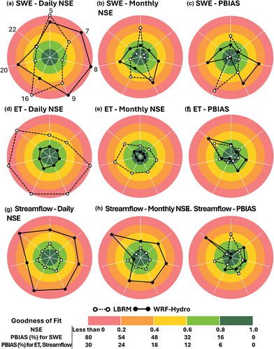
Figure 3. Time series of observed and simulated (both WRF-Hydro and LBRM-CC) SWE (top row), ET (middle row), and streamflow (bottom row) at daily (left column) and monthly (middle column) time steps, and monthly biases (right column) from Lake Michigan sub-basin 5. Similar results for all other sub-basins are included in the Supplementary material.

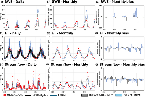
When evaluating the performance in simulating ET, WRF-Hydro demonstrated superior results compared to LBRM-CC in both daily and monthly NSE (Fig. 2). Specifically, the average daily NSE values for the selected sub-basins were 0.74 for WRF-Hydro and −1.49 for LBRM-CC. Both models showed improved NSE values at the monthly scale compared to the daily scale, with average monthly NSEs of 0.88 for WRF-Hydro and 0.59 for LBRM-CC across the sub-basins. LBRM-CC exhibited a significant improvement in NSE values from daily to monthly scale, likely due to the smoothing effect that diminished large daily fluctuations when aggregated to monthly values (Fig. 3). The lower performance of LBRM-CC in estimating ET can be attributed to its ET calculation algorithm, which utilizes the Clausius-Clapeyron relationship (details can be found in the Supplementary material, Equations S1 to S9). The calculation involves several empirical parameters defined by the user to estimate potential ET (Lofgren et al. 2011, Lofgren and Rouhana 2016). Additionally, the ET estimation in LBRM-CC is influenced by the water content in both the upper and lower soil zones. Since LBRM-CC is a conceptual and lumped model, its results heavily rely on the selection of parameters and initial conditions. To gain further insights, we performed a global sensitivity analysis of the model parameters to identify the most influential ones for LBRM-CC modeling (see the Supplementary material, Text 2). This analysis confirmed the significant role of the “T base” parameter associated with the base temperature in accurately simulating ET in LBRM-CC (Lofgren and Rouhanaa 2016). Detailed discussions on the outcomes of the sensitivity analysis for LBRM-CC’s model parameters can be found in the Discussion section.

The performance of simulating streamflow exhibited contrasting trends compared to ET simulations, with LBRM-CC surpassing WRF-Hydro in terms of daily and monthly NSE (Fig. 2). For instance, LBRM-CC demonstrated daily NSE ranges from 0.63 to 0.77 and monthly NSE ranges from 0.67 to 0.86. In contrast, WRF-Hydro exhibited NSE ranges of 0.03 to 0.41 for daily streamflow and 0.07 to 0.82 for monthly streamflow. This outcome can be attributed to the different calibration strategies employed by the two models. LBRM-CC utilizes a local calibration approach, tuning 10 model parameters for each individual sub-basin focusing on the modeling accuracy of the streamflow (Croley and He 2005, Lofgren and Rouhanaa 2016). Thus, we can see that the substantial variations in daily ET simulated by LBRM-CC did not significantly impact the daily streamflow simulation (Fig. 3). On the other hand, WRF-Hydro adopts a regional calibration approach, where model parameters are determined based on the spatial characteristics of the region (e.g. lower values of surface retention depth in steep slope or surface roughness assigned by land cover types; Yucel et al. 2015, Naabil et al. 2017). Previous studies have also reported that lumped models often exhibit higher accuracy in simulating specific variables of interest compared to complex advanced models (Kumar et al. 2015, Kumari et al. 2021, Mai et al. 2022).

3.2 Subsurface components: soil moisture

WRF-Hydro performed better than LBRM-CC in terms of accurately simulating soil moisture (Figs. 4 and 5). Due to the difficulties of direct comparison (Fig. S3), we used the PBIAS to measure the overall bias or tendency of the simulated soil moisture. In comparison with GLEAM and SMAP, WRF-Hydro’s average PBIAS values for the first soil layer were 17.2% and 21.2%, while those for LBRM-CC were 64.9% and 73.1%, respectively. Overall, LBRM-CC showed large variations, while WRF-Hydro demonstrated similar trends to GLEAM and SMAP. The average PBIAS values for soil layers 2, 3, and 4 of WRF-Hydro were 15.0%, 11.6%, and 10.5%, respectively, while for soil layer 2 of LBRM it was 82.3%. In the selected sub-basins, SMAP showed average surface soil moisture values ranging from 0.25 to 0.41 m³/m³, and GLEAM indicated average surface and root zone soil moisture values ranging from 0.29 to 0.37 m³/m³. For all soil layers, WRF-Hydro and LBRM-CC showed average soil moisture values from 0.22 to 0.28 m³/m³ and from 0.0003 to 0.47 m³/m³, respectively. As reported in a previous study (Xu et al. 2021), soil moisture contents in the western part of the Lake Michigan basin ranged from 0.1 to 0.4 m³/m³, based on in situ observations from 2015 to 2019.

Figure 4. The performance statistics of WRF-Hydro and LBRM-CC in simulating subsurface components including soil moisture in different soil layers for the seven sub-basins located in the Lake Michigan basin.

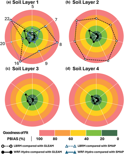
Figure 5. Time series of simulated and reference (GLEAM and SMAP) soil moisture (as a volumetric proportion) in different conceptual subsurface layers in the LBRM-CC (left) and WRF-Hydro (right) from Lake Michigan sub-basin 5. GLEAM and SMAP soil moisture at the surface layer (0–5 cm) was compared with each model’s soil moisture output at soil layer #1. GLEAM soil moisture at the root zone (5 cm – vary) was compared with soil moisture outputs at soil layers #2, #3, and #4. WRF-Hydro provided soil moisture and soil water depth. LBRM-CC only provided soil water depth, which was converted to soil moisture.

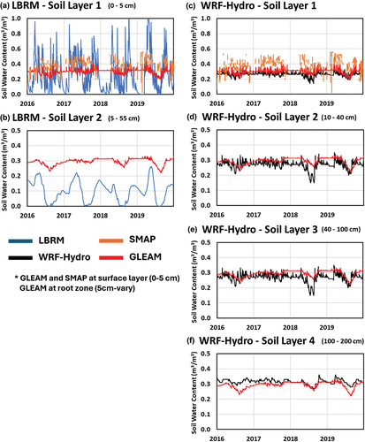
In the case of WRF-Hydro, the PBIAS values for all soil layers exhibited consistency across all selected sub-basins (Fig. 4), and the simulated values closely followed the reference trends observed in GLEAM data (Fig. 5; and the time-series comparison for other sub-basins can be found in the Supplementary material, Figs. S8 to 14), indicating that the model’s parameterization related to soil moisture is reasonable, physically-based, and spatially distributed (Xiang et al. 2017, Sofokleous et al. 2023). Meanwhile, in the case of LBRM-CC, the PBIAS values for soil moisture at soil layer 1 varied depending on the locations, while those at soil layer 2 remained consistent. Through the model parameter sensitivity analysis conducted for LBRM-CC outputs, it was found that a single model parameter related to surface flow had the most significant influence on soil moisture in soil layer 1 (or upper zone soil moisture) (Figs. S6 and S7), indicating substantial impacts of this parameter in the soil moisture modeling at soil layer 1, which likely contributes to the spatial inconsistency in the simulated soil moisture of LBRM-CC at this layer. On the other hand, multiple model parameters related to interflow and deep percolation were identified as the most influential factors for the simulated soil moisture in soil layer 2 (or lower zone soil moisture), which denotes significant interactions with other model parameters in the modeling of soil moisture in this layer. As a result, the individual parameters had relatively minor effects on soil moisture in the lower zone compared to the upper zone.

3.3 Groundwater components: baseflow

Both WRF-Hydro and LBRM-CC exhibited similar trends to the reference baseflow data, with correlation coefficients greater than 0.5 between the reference baseflow and simulated ones at all sub-basins (Fig. 6). The PBIAS ranges for WRF-Hydro and LBRM-CC were 15.8% to 58.3% (mean of 30.6%) and 12.4% to 42.1% (mean of 30.1%), respectively. Despite having different conceptualizations of underground layers, both models performed well in capturing the characteristics of the reference baseflow data. However, the simulated baseflow of WRF-Hydro displayed inconsistent trends between sub-basins, with underestimation of the baseflow in sub-basins 5 and 9. This inconsistency is likely due to the highly conceptualized formulation of the groundwater bucket model in WRF-Hydro, which relies on four empirical parameters (i.e. the bucket model coefficient, the bucket model exponent, the initial depth of water in the bucket model, and the maximum storage in the bucket before “spilling” occurs; Gochis et al. 2020). Fine-tuning these parameter values through model calibration would improve the accuracy of the groundwater bucket models. On the other hand, LBRM-CC displayed large variations in baseflow at sub-basins 16 and 22, while exhibiting smoother curves at sub-basins 5 and 20. The results of the model parameter sensitivity analysis for LBRM-CC outputs indicated that a single parameter related to groundwater had the most significant influence on baseflow (Figs. S6 and S7). This suggests that the simulated baseflow in LBRM-CC heavily relies on this parameter, which controls the shape of the baseflow hydrograph, highlighting the importance of selecting appropriate model parameters in LBRM-CC.

Figure 6. The simulation results of the groundwater component of WRF-Hydro and LBRM-CC at the selected sub-basins in the Lake Michigan basin compared to the reference data from baseflow separation, which was conducted using the baseflow index (BFI) standard method for the observed USGS streamflow data.

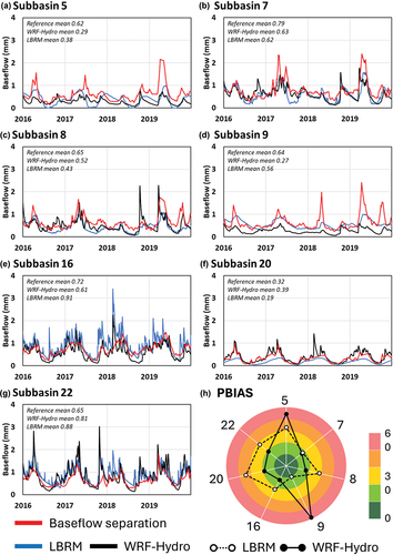
The selected sub-basins exhibited subsurface or baseflow dominance, with an average runoff ratio (i.e. the proportion of total runoff to total rainfall) of 30% and a baseflow index (i.e. the proportion of baseflow to total runoff) of 68% (Table 2). These values align with findings from previous studies (Fry et al. 2014, Mei et al. 2023) and indicate the substantial contribution of baseflow to streamflow (Neff et al. 2005). The runoff ratio is affected by various factors such as physical characteristics (e.g. slope, land use, and soil), rainfall characteristics (e.g. intensity and duration), hydrological conditions, and anthropogenic factors such as artificial storage created by water control structures (Yadav et al. 2007, Munyaneza et al. 2012, Kult et al. 2014, Shin et al. 2023a). The low runoff ratio suggests that rainfall events have limited influence on the discharge at the basin outlet, potentially due to significant impacts from the subsurface and groundwater processes. It has been noted in previous research that basins dominated by baseflow often exhibit lower accuracy in streamflow simulation (Fry et al. 2014, Mei et al. 2023), which could explain the lower performance of WRF-Hydro in this study. To improve the representation of groundwater processes, the simple conceptualization employed in WRF-Hydro could be enhanced through integration with more advanced modules (Rummler et al. 2022, Mei et al. 2023, Sofokleous et al. 2023).

Table 2. Summary of the average runoff ratio and baseflow index of the selected sub-basins in the Lake Michigan basin. P, R, and B represent precipitation, runoff, and baseflow, respectively.

Sub-basin	Item	P (mm/year)^a	R (mm/year)	B (mm/year)^b	Runoff ratio (%)^c	Baseflow index (%)
5	Observation	–	460.0	256.0	–	55.7
	WRF-Hydro	1325.2	482.7	129.5	36.4	26.8
	LBRM-CC	1084.2	391.9	167.4	36.1	42.7
7	Observation	–	467.6	344.2	–	73.6
	WRF-Hydro	1330.8	405.3	272.9	30.5	67.3
	LBRM-CC	1147.6	436.3	276.4	38.0	63.3
8	Observation	–	442.3	284.2	–	64.3
	WRF-Hydro	1354.8	388.0	222.5	28.6	57.3
	LBRM-CC	1191.9	403.9	185.3	33.9	45.9
9	Observation	–	417.3	277.8	–	66.6
	WRF-Hydro	1272.6	374.5	114.5	29.4	30.6
	LBRM-CC	1214.2	364.3	243.5	30.0	66.9
16	Observation	–	396.8	311.8	–	78.6
	WRF-Hydro	1422.2	431.9	258.6	30.4	59.9
	LBRM-CC	1385.2	410.2	385.0	29.6	93.8
20	Observation	–	214.9	137.2	–	63.9
	WRF-Hydro	1271.9	209.9	163.8	16.5	78.0
	LBRM-CC	1271.5	237.5	79.1	18.7	33.3
22	Observation	–	388.1	290.2	–	74.8
	WRF-Hydro	1314.6	464.0	344.7	35.3	74.3
	LBRM-CC	1213.2	397.3	382.4	32.7	96.3

^aPrecipitation data for WRF-Hydro and LBRM-CC is ERA5 and GHCN, respectively.

^bBaseflow for observations is derived by the baseflow separation method applied for the observed runoff.

^cRunoff ratio is R/P*100; baseflow index is calculated as B/R*100.

4 Discussion

4.1 Performance of the hydrological models

The overall performance of LBRM-CC in simulating SWE was relatively better than that of WRF-Hydro. However, there was inconsistency in performance between sub-basins, likely due to the fact that the simulated SWE was controlled by a single parameter, with the effects of other parameters being negligible (Figs. S6 and S7). It is important to carefully consider the values of model parameters in LBRM-CC to avoid unrealistic modeling results. Even though monthly fluctuations in simulated ET were relatively small, there were large variations on the daily scale and poor performance statistics (Figs. 2 and 3). The performance of hydrological models often improves when evaluated at a monthly scale compared to a daily scale because (1) daily noise in both input data and simulated values is smoothed out when aggregated to a monthly scale, resulting in a clear signal and improved model performance, and (2) the time scale resolutions in a model become finer, making it difficult to reproduce accurate timing of hydrological processes in a model (Engel et al. 2007, Moriasi et al. 2007, 2015). The sensitivity analysis of model parameters revealed that ET is particularly sensitive to some specific parameters (Figs. S6 and S7). A parameter related to the base temperature (i.e. Tbase) was identified as the most influential parameter for the average and variance of simulated ET in LBRM-CC. Parameters associated with percolation between the upper soil zone and lower soil zone, as well as between the lower soil zone and groundwater zone, have significant impacts on the regulation of soil water levels in the conceptual tanks within LBRM-CC. The values of ET in LBRM-CC are closely linked to the storage of soil water in the first and second tanks. The amount of ET at each tank is directly influenced by conceptual parameters (e.g. USZevap and LSZevap), as these parameters are multiplied by the soil water storage values (Equations S1.1 and S1.2).

Although this study did not specifically examine the sensitivity of initial conditions (e.g. initial water storage in the upper soil zone, lower soil zone, and groundwater zone), these values are also crucial for modeling accuracy (Croley and He 2005). Local calibration of the models can yield good results for specific variables in particular regions and periods, but it may lead to unrealistic modeling outcomes beyond the calibration period or for unaccounted variables (Seiller et al. 2012, Mai et al. 2022). Due to the inaccurate representation of physical processes, employing these models to predict uncertain future conditions becomes problematic (Niel et al. 2003). For example, the changes in rainfall and temperature may alter runoff responses, while the responses of other variables such as ET, SWE, soil moisture, and groundwater might not be the same and could affect the runoff responses, as these are not targeted in the calibration process. This prompts the need for further examination of hydrological model responses to climate changes in future studies.

Can we use a lumped model for operational purposes, given its good performance in simulating streamflow, despite its unrealistic representation of other physical processes such as ET, soil moisture, and groundwater? The simple lumped model demonstrates good performance in simulating streamflow due to localized parameter calibration, and its computational efficiency makes it suitable for large spatial and temporal scales (Fry et al. 2014, Gaborit et al. 2017). Historically, LBRM-CC has been used for simulating runoff over monthly or inter-annual time scales for more than two decades; thus, it is not expected to exhibit good performance in simulating other hydrological components. However, under changing climate conditions, the potential for unrealistic representation of other variables can be problematic. To address the issue of unrealistic representation of other variables, careful consideration of parameter ranges is necessary. Additionally, advanced calibration techniques or ensemble modeling can be explored to improve the accuracy of modeling results (Mai 2023, Shin et al. 2023b).

The performance of complex or advanced models, such as WRF-Hydro, can vary depending on the specific application and scale of analysis. In the case of the WRF-Hydro model, it demonstrated good performance in simulating both surface and subsurface components, although it exhibited relatively lower performance in streamflow simulation. The model also exhibited a consistent level of performance across the entire modeling domain, and even its simplified conceptualization of groundwater components matched well with the reference baseflow data.

This study employed different forcings than those used to calibrate the NWMv2.1. The use of different climate forcings in this study, compared to the NWMv2.1, may have resulted in lower performance in streamflow simulation specifically in the study area. The climate forcings, such as precipitation and temperature data, play a crucial role in driving hydrological models, and differences in the input data can impact model performance. In this study, the model parameter configuration for WRF-Hydro was based on the NWMv2.1, which incorporated the expansion of the Great Lakes basin into Canada and included calibration over the entire Great Lakes basin (Mason et al. 2019). At the regional scale, further modifications may be necessary to adjust the model parameters through the calibration process for improving the accuracy of streamflow simulation in the study area. Future studies may try advanced techniques such as data assimilation (Yucel et al. 2015) and machine learning algorithms (Cho and Kim 2022) for model calibration to effectively improve model accuracy.

Nonetheless, advanced models like WRF-Hydro can be valuable as reference tools to represent physical processes and interactions in the hydrological systems. Process-based models are based on fundamental physical principles rather than region-specific parameterizations, making them more transferable to different regions and catchments. This inherent characteristic also renders them suitable for various scenario applications (e.g. land-use or climate changes) (Fatichi et al. 2016, Abbaszadeh et al. 2020, Pal et al. 2023). In addition, they provide spatially distributed outputs considering spatial variations of land surface, soil types, and topography, which is particularly useful for large and heterogeneous watersheds such as the Great Lakes region.

We compared the model performance between this study and a previous model intercomparison study for the entire Great Lakes basin (Mai et al. 2022; hereafter referred to GRIP-GL) (see the Supplementary material, Table S3). In terms of the performance of LBRM-CC, we found that the performance of flow and surface soil moisture simulations between this study and GRIP-GL was similar, while that of ET and SWE showed substantial differences. This difference can be attributed to the different reference datasets used in each study. For instance, the two studies utilized the same reference datasets for flow and surface soil moisture (USGS flow and GLEAM surface soil moisture), which resulted in similar performance between this study and GRIP-GL. Meanwhile, different reference datasets were adopted for ET and SWE (e.g. MODIS ET for this study vs. GLEAM ET for GRIP-GL, GHCN SWE for this study vs. ERA5 SWE for GRIP-GL), leading to substantial differences in performance between the two studies. WRF-Hydro was employed for the first time in this study for model intercomparison; therefore, the performance of WRF-Hydro cannot be directly compared to GRIP-GL. Nonetheless, the results of GRIP-GL’s more complex and advanced models were consistent with those of WRF-Hydro, showing low performance for flow simulations, but good performance for ET and surface soil moisture simulations (see the Supplementary material, Table S3). Though there are many differences between the two studies, such as the simulation domain, comparison period, model inputs, calibration techniques, and validation datasets, this study aligns with GRIP-GL and adds more information on the state-of-the-art land surface model, which has never been examined before. In this study, we did not recommend a specific model for water management in the Great Lakes region. Instead, we identified the capabilities and limitations of each model based on comprehensive evaluations of various hydrological processes. We believe the findings of this study will provide useful information for water managers in the Great Lakes basins since we examined the two models with their original operational settings (e.g. the same configuration and model parameters used by the operators) rather than customizing or modifying them. Hence, the strengths and weaknesses identified in this study can be used to improve both models.

4.2 Seasonal and long-term water balance

Four years of simulation is a relatively short period to capture natural variability. It is noteworthy, however, that the two models were not calibrated and validated during the evaluation period selected in this study (Table S1), which comprised recent wet periods that may have a significant impact on the regional water balance. An earlier study (Wilcox et al. 2007) identified a period of 160 ± 40 years as capable of capturing a natural rise-and-fall pattern in Lake Michigan–Huron using a reconstructed (pre-historical) hydrograph of lake level changes over the past 4700 years. Nevertheless, simulations of hundreds of years are beyond our capacity, especially when it comes to the more computationally expensive and complex model, WRF-Hydro. Due to the short simulation periods in this study, the natural variability of the study area is not captured; however, the goal is to explore various hydrological responses of two important operational models during recent wet periods, a period in which both models have not been evaluated previously. The limited time frame gives us the opportunity to obtain data from a variety of sources for evaluating the different hydrological components.

To investigate the implications of the seasonal and long-term water balance modeling, we compared the performance of the two models in simulating seasonal and long-term hydrological components compared to the reference datasets (Fig. 7). We calculated area-weighted averages of streamflow, baseflow, ET, SWE, and soil moisture for the selected sub-basins using reference datasets and simulation results. The hydrological simulations of both models performed better at coarse temporal scales than at finer temporal scales, due to cancelling out noise and bias in finer temporal scales. For instance, LBRM-CC showed substantial differences in ET performances between daily and other temporal scales (monthly, seasonal, and long-term scales) (Figs. 2 and 7). The simulated ET showed large fluctuations, with poor performance on a daily scale, but the performance greatly improved on monthly and seasonal scales. In addition, LBRM-CC performed substantially better on the seasonal and long-term scale for other variables such as streamflow, baseflow, and SWE, indicating consistent patterns with the reference datasets; however, the soil moisture simulations displayed unrealistic representations, significantly underestimating the reference datasets (Fig. 7). Seasonal and long-term WRF-Hydro performances were improved compared to performances evaluated daily or monthly. The warm season ET and soil moisture simulations using WRF-Hydro showed a slight underestimation but demonstrated reasonable performances consistent with the reference datasets; however, SWE simulations showed large underestimations, causing spring flow to be underestimated as well. On a seasonal and long-term scale, LBRM-CC well captured streamflow, warm season ET, and SWE better than WRF-Hydro, while WRF-Hydro did cold season ET and soil moisture simulations better than LBRM-CC.

Figure 7. The monthly and seasonal average flow (a), ET (b), SWE (c), and soil moisture (d) from reference and simulations. The area-weighted values were calculated based on the reference dataset and simulated results for the selected seven sub-basins. Monthly values are represented starting from May. The warm season mean is calculated using the average from May to October, and the cold season mean is calculated based on the rest of the year. Line plots in plot (a) show baseflow, and those in (d) show various soil moisture values in different soil layers. SWE was considered only for December, January, and February.

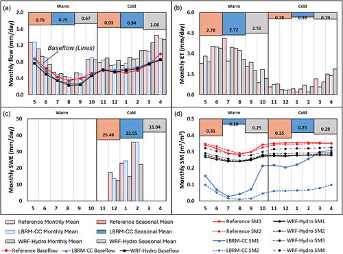
Both models captured seasonal and long-term trends of flow and ET well. Streamflow increased during spring due to snowmelt, peaked in April, and decreased during summer with the lowest flow in August. In the cold season, streamflow was greater than in the warm season due to lower ET and more snow. Baseflow decreased in summer and increased in spring, showing substantial contributions from groundwater to total runoff, with an average baseflow index of 70%. Though the two models adopted similar conceptual representations of groundwater processes (e.g. simple groundwater bucket model with empirical parameters), the groundwater simulations were consistent with the reference dataset. The model accuracy could be improved by further calibration of empirical parameters or employing more advanced groundwater modules. There were significant seasonal differences in ET, with warm-season ET exceeding 3.5 times cold-season ET. Both models underestimated the peak ET in July and overestimated it through September to November, while the overall amount of seasonal ET was well captured. Monthly SWE increased from December to February; LBRM-CC well captured the overall amount of SWE, while WRF-Hydro underestimated it, which resulted in lower spring flow. Studies have suggested that snow processes in WRF-Hydro can be enhanced by fine-tuning algorithms of the land surface model, such as snow albedo schemes (Abolafia-Rosenzweig et al. 2022, Liu et al. 2022) and soil freeze–thaw processes (Yang et al. 2023). Soil moisture in the cold season was greater than that in the warm season. In WRF-Hydro and reference datasets, soil moisture remained high and stable during the cold season due to lower ET and snow accumulation and decreased during the warm season due to higher ET rates and increased vegetation. LBRM-CC, however, produced unrealistic soil moisture simulations, and further calibration should be considered to improve the accuracy.

5 Conclusions

In this study, we conducted a comprehensive evaluation of candidate models for operational water balance and water supply simulation and forecasting across Earth’s largest lake system. This study compared the simulated outputs with observed data from ground-based stations and remotely sensed images and validated the simulated surface variables (e.g. snow water equivalent, evapotranspiration, and streamflow), subsurface variables (e.g. soil moisture at different layers), and groundwater components to improve the understanding of these models. The results indicated that LBRM-CC outperformed WRF-Hydro in simulating SWE and streamflow, while WRF-Hydro exhibited better performance in simulating ET and soil moisture. The simple lumped model demonstrated good performance in streamflow simulation due to localized parameter calibration. However, this simplicity resulted in unrealistic representations of other variables and spatial inconsistencies. Therefore, careful consideration of model parameters is crucial to address these issues. WRF-Hydro showed consistent performance across the entire modeling domain, although its performance in streamflow simulation was relatively lower compared to LBRM-CC. Further calibration would be necessary to improve the accuracy of the streamflow simulations in the Great Lakes region. However, they can serve as valuable reference tools for providing a more comprehensive and detailed understanding of hydrological processes. This detailed representation of physical processes and interactions in the hydrological system can be particularly useful for conducting various scenario analyses, which are essential for water resource management planning. Here, we first incorporated WRF-Hydro, the state-of-the-art land surface hydrological model, into the comprehensive evaluation of its performance with LBRM-CC in representing Great Lakes hydrology. In addition, our evaluation covered a wide range of hydrological components, from surface to groundwater, which is not well documented in previous studies. The findings of this study contribute to our understanding of these two hydrological models and test the potential of the state-of-the-art land surface model in simulating Great Lakes hydrology. By assessing multiple hydrological processes, we gain valuable insights into the strengths and limitations of both models, which is crucial for making informed decisions in water resource management and operational water supply forecasting in the Great Lakes region.

Acknowledgements

This work was supported by the Framework for Resilient Great Lakes Restoration Initiative (GLRI) Investments Project through a collaborative partnership between the Cooperative Institute for Great Lakes Research (CIGLR), the National Oceanic and Atmospheric Administration (NOAA), the United States Army Corps of Engineers (USACE), and the United States Geological Survey (USGS).

Disclosure statement

No potential conflict of interest was reported by the author(s).

Supplementary material

Supplemental data for this article can be accessed online at https://doi.org/10.1080/02626667.2024.2378100

Additional information

Funding

Funding was awarded to CIGLR through the NOAA Cooperative Agreement with the University of Michigan [CIGLR Award No. NA22OAR4320150]. This is CIGLR contribution 1247 and NOAA Great Lakes Environmental Research Laboratory (GLERL) Contribution 2051. ADG was partially supported through the NSF Global Centers program [NSF Award No. 2330317].

References

- Abbaszadeh, P., Gavahi, K., and Moradkhani, H., 2020. Multivariate remotely sensed and in-situ data assimilation for enhancing community WRF-Hydro model forecasting. Advances in Water Resources, 145, 103721. doi:10.1016/j.advwatres.2020.103721.
- Abolafia‐Rosenzweig, R., et al., 2022. Evaluation and optimization of snow albedo scheme in Noah‐MP land surface model using in situ spectral observations in the Colorado Rockies. Journal of Advances in Modeling Earth Systems, 14 (10), e2022MS003141. doi:10.1029/2022MS003141.
- Ala-aho, P., et al., 2017. Integrated surface-subsurface model to investigate the role of groundwater in headwater catchment runoff generation: a minimalist approach to parameterisation. Journal of Hydrology, 547, 664–677. doi:10.1016/j.jhydrol.2017.02.023.
- Archfield, S.A., et al., 2015. Accelerating advances in continental domain hydrologic modeling. Water Resources Research, 51 (12), 10078–10091. doi:10.1002/2015WR017498.
- Arsenault, R., Brissette, F., and Martel, J.L., 2018. The hazards of split-sample validation in hydrological model calibration. Journal of Hydrology, 566, 346–362. doi:10.1016/j.jhdrol.2018.09.027.
- Bajracharya, A.R., et al., 2023. Process based calibration of a continental-scale hydrological model using soil moisture and streamflow data. Journal of Hydrology: Regional Studies, 47, 101391. doi:10.1016/j.ejrh.2023.101391.
- Barlow, P.M., et al., 2015. U.S. Geological Survey groundwater toolbox, a graphical and mapping interface for analysis of hydrologic data (version 1.0): user guide for estimation of base flow, runoff, and groundwater recharge from streamflow data. Reston, VA: US Geological Survey. doi:10.3133/tm3B10.
- Bingeman, A.K., Kouwen, N., and Soulis, E.D., 2006. Validation of the hydrological processes in a hydrological model. Journal of Hydrologic Engineering, 11 (5), 451–463. doi:10.1061/(ASCE)1084-0699(2006)11:5(451).
- Biondi, D., et al., 2012. Validation of hydrological models: conceptual basis, methodological approaches and a proposal for a code of practice. Physics and Chemistry of the Earth, Parts A/B/C, 42–44, 70–76. doi:10.1016/J.PCE.2011.07.037.
- Charusombat, U., et al., 2018. Evaluating and improving modeled turbulent heat fluxes across the North American Great Lakes. Hydrology and Earth System Sciences, 22 (10), 5559–5578. doi:10.5194/HESS-22-5559-2018.
- Cho, K. and Kim, Y., 2022. Improving streamflow prediction in the WRF-Hydro model with LSTM networks. Journal of Hydrology, 605, 127297. doi:10.1016/j.jhydrol.2021.127297.
- Clark, M.P., et al., 2015. Improving the representation of hydrologic processes in Earth System Models. Water Resources Research, 51 (8), 5929–5956. doi:10.1002/2015WR017096.
- Costa, D., Zhang, H., and Levison, J., 2021. Impacts of climate change on groundwater in the Great Lakes Basin: a review. Journal of Great Lakes Research, 47 (6), 1613–1625. doi:10.1016/J.JGLR.2021.10.011.
- Croley, T.E., 1983. Great Lake basins (USA-Canada) runoff modeling. Journal of Hydrology, 64 (1–4), 135–158. doi:10.1016/0022-1694(83)90065-3.
- Croley, T.E. and He, C., 2005. Distributed-parameter large basin runoff model. I: model Development. Journal of Hydrologic Engineering, 10 (3), 173–181. doi:10.1061/(asce)1084-0699(2005)10:3(173).
- Devia, G.K., Ganasri, B.P., and Dwarakish, G.S., 2015. A review on hydrological models. Aquatic Procedia, 4, 1001–1007. doi:10.1016/J.AQPRO.2015.02.126.
- EC and USEPA (Environment Canada and the United States Environmental Protection Agency). 2003. State of the Great Lakes 2003. Cat No. En40-11/35-2003E. EPA 905-R-03-004. Availbale from: https://archive.epa.gov/solec/web/pdf/state_of_the_great_lakes_2003_summary_report.pdf [Accessed 23 July 2024].
- Ek, M.B., et al., 2003. Implementation of Noah land surface model advances in the National Centers for environmental prediction operational mesoscale Eta model. Journal of Geophysical Research: Atmospheres, 108 (D22), 8851. doi:10.1029/2002JD003296.
- Engel, B., et al., 2007. A hydrologic/water quality model applicati1. Journal of the American Water Resources Association, 43 (5), 1223–1236. doi:10.1111/j.1752-1688.2007.00105.x.
- EPA (United States Environmental Protection Agency). 2023. Facts and figures about the great lakes. https://www.epa.gov/greatlakes/facts-and-figures-about-great-lakes [ Accessed 30 May 2023].
- Erler, A.R., et al., 2019. Evaluating climate change impacts on soil moisture and groundwater resources within a Lake-Affected Region. Water Resources Research, 55 (10), 8142–8163. doi:10.1029/2018WR023822.
- Fatichi, S., et al., 2016. An overview of current applications, challenges, and future trends in distributed process-based models in hydrology. Journal of Hydrology, 537, 45–60. doi:10.1016/j.jhydrol.2016.03.026.
- Fry, L.M., Apps, D., and Gronewold, A.D., 2020. Operational Seasonal water supply and water level forecasting for the laurentian Great Lakes. Journal of Water Resources Planning and Management, 146 (9). doi:10.1061/(asce)wr.1943-5452.0001214.
- Fry, L.M., et al., 2014. The Great Lakes Runoff Intercomparison Project phase 1: lake Michigan (GRIP-M). Journal of Hydrology, 519, 3448–3465. doi:10.1016/j.jhydrol.2014.07.021.
- Gaborit, É., et al., 2017. Great Lakes Runoff Inter-comparison Project, phase 2: lake Ontario (GRIP-O). Journal of Great Lakes Research, 43 (2), 217–227. doi:10.1016/j.jglr.2016.10.004.
- Garavaglia, F., et al., 2017. Impact of model structure on flow simulation and hydrological realism: from a lumped to a semi-distributed approach. Hydrology and Earth System Sciences, 21 (8), 3937–3952. doi:10.5194/hess-21-3937-2017.
- Gesch, D.B., et al., 2002. The national elevation data set. Photogrammetric Engineering & Remote Sensing, 68 (1), 5–11.
- Gochis, D.J., et al., 2020. The NCAR WRF-hydro modeling system technical description. Boulder, CO, USA: University Corporation for Atmospheric Research.
- Gochis, J. and Chen, F., 2003. Hydrological enhancements to the community Noah Land surface model. Boulder, CO, USA: University Corporation for Atmospheric Research. doi:10.5065/D60P0X00.
- Gronewold, A.D., Anderson, E.J., and Smith, J., 2019. Evaluating operational hydrodynamic models for real-time simulation of evaporation from large Lakes. Geophysical Research Letters, 46 (6), 3263–3269. doi:10.1029/2019GL082289.
- Gronewold, A.D., et al., 2011. An appraisal of the Great Lakes advanced hydrologic prediction system. Journal of Great Lakes Research, 37 (3), 577–583. doi:10.1016/j.jglr.2011.06.010.
- Gronewold, A.D., et al., 2013. Coasts, water levels, and climate change: a Great Lakes perspective. Climatic Change, 120 (4), 697–711. doi:10.1007/S10584-013-0840-2/FIGURES/7.
- Hersbach, H., et al., 2020. The ERA5 global reanalysis. Quarterly Journal of the Royal Meteorological Society, 146 (730), 1999–2049. doi:10.1002/QJ.3803.
- Holman, K.D., et al., 2012. Improving historical precipitation estimates over the Lake Superior basin. Geophysical Research Letters, 39 (3). doi:10.1029/2011GL050468.
- Homer, C., et al., 2015. Completion of the 2011 national Land cover database for the conterminous United States–representing a decade of land cover change information. Photogrammetric Engineering & Remote Sensing, 81 (5), 345–354. doi:10.14358/PERS.81.5.345.
- Hong, Y., et al., 2022. Evaluation of gridded precipitation datasets over international basins and large lakes. Journal of Hydrology, 607, 127507. doi:10.1016/J.JHYDROL.2022.127507.
- Hrachowitz, M., et al., 2014. Process consistency in models: the importance of system signatures, expert knowledge, and process complexity. Water Resources Research, 50 (9), 7445–7469. doi:10.1002/2014WR015484.
- Hunter, T.S., et al., 2015. Development and application of a North American Great Lakes hydrometeorological database — part I: precipitation, evaporation, runoff, and air temperature. Journal of Great Lakes Research, 41 (1), 65–77. doi:10.1016/J.JGLR.2014.12.006.
- Institute of Hydrology, 1980. Low Flow Studies. Wallingford, UK: Institute of Hydrology.
- Kirchner, J.W., 2006. Getting the right answers for the right reasons: linking measurements, analyses, and models to advance the science of hydrology. Water Resources Research, 42 (3). doi:10.1029/2005WR004362.
- Kult, J.M., et al., 2014. Regionalization of hydrologic response in the Great Lakes basin: considerations of temporal scales of analysis. Journal of Hydrology, 519, 2224–2237. doi:10.1016/J.JHYDROL.2014.09.083.
- Kumar, A., et al., 2015. Identification of the best multi-model combination for simulating river discharge. Journal of Hydrology, 525, 313–325. doi:10.1016/j.jhydrol.2015.03.060.
- Kumari, N., et al., 2021. Identification of suitable hydrological models for streamflow assessment in the Kangsabati River Basin, India, by using different model selection scores. Natural Resources Research, 30 (6), 4187–4205. doi:10.1007/S11053-021-09919-0/FIGURES/7.
- Li, L., et al., 2017. Evaluating the present annual water budget of a Himalayan headwater river basin using a high-resolution atmosphere-hydrology model. Journal of Geophysical Research, 122 (9), 4786–4807. doi:10.1002/2016JD026279.
- Liu, L., Menenti, M., and Ma, Y., 2022. Evaluation of albedo schemes in WRF coupled with Noah-MP on the Parlung No. 4 Glacier. Remote Sensing, 14 (16), 3934. doi:10.3390/rs14163934.
- Liu, Y. and Gupta, H.V., 2007. Uncertainty in hydrologic modeling: toward an integrated data assimilation framework. Water Resources Research, 43 (7), 7401. doi:10.1029/2006WR005756.
- Lofgren, B.M., et al., 2013. Methodological approaches to projecting the hydrologic impacts of climate change. Earth Interactions, 17 (22), 1–19. doi:10.1175/2013EI000532.1.
- Lofgren, B.M. and Gronewold, A.D., 2013. Reconciling alternative approaches to projecting hydrologic impacts of climate change. Bulletin of the American Meteorological Society, 94 (10), ES133–ES135. doi:10.1175/BAMS-D-13-00037.1.
- Lofgren, B.M., Hunter, T.S., and Wilbarger, J., 2011. Effects of using air temperature as a proxy for potential evapotranspiration in climate change scenarios of Great Lakes basin hydrology. Journal of Great Lakes Research, 37, 744–752. doi:10.1016/j.jglr.2011.09.006.
- Lofgren, B.M. and Rouhanaa, J., 2016. Physically plausible methods for projecting changes in Great Lakes Water Levels under climate change scenarios. Journal of Hydrometeorology, 17 (8), 2209–2223. doi:10.1175/JHM-D-15-0220.1.
- López López, P., et al., 2017. Calibration of a large-scale hydrological model using satellite-based soil moisture and evapotranspiration products. Hydrology and Earth System Sciences, 21 (6), 3125–3144. doi:10.5194/hess-21-3125-2017.
- Mai, J., et al., 2021. Great Lakes Runoff intercomparison project phase 3: lake Erie (GRIP-E). Journal of Hydrologic Engineering, 26 (9). doi:10.1061/(asce)he.1943-5584.0002097.
- Mai, J., et al., 2022. The Great Lakes Runoff Intercomparison Project Phase 4: the Great Lakes (GRIP-GL). Hydrology and Earth System Sciences, 26 (13), 3537–3572. doi:10.5194/hess-26-3537-2022.
- Mai, J., 2023. Ten strategies towards successful calibration of environmental models. Journal of Hydrology, 620, 129414. doi:10.1016/J.JHYDROL.2023.129414.
- Martens, B., et al., 2017. GLEAM v3: satellite-based land evaporation and root-zone soil moisture. Geoscientific Model Development, 10, 1903–1925. doi:10.5194/gmd-10-1903-2017.
- Mason, L.A., et al., 2019. New transboundary hydrographic data set for advancing regional hydrological modeling and water resources management. Journal of Water Resources Planning and Management, 145 (6). doi:10.1061/(asce)wr.1943-5452.0001073.
- McKay, L., et al., 2012. US Environmental Protection Agency. Washington, DC: National Operational Hydrologic Remote Sensing Center.
- Mei, Y., et al., 2023. Can hydrological models benefit from using global soil moisture, evapotranspiration, and Runoff products as calibration targets? Water Resources Research, 59 (2). doi:10.1029/2022WR032064.
- Menne, M.J., et al., 2012. An overview of the global historical climatology network-daily database. Journal of Atmospheric and Oceanic Technology, 29 (7), 897–910. doi:10.1175/JTECH-D-11-00103.1.
- Miller, D.A. and White, R.A., 1998. A conterminous united states multilayer soil characteristics dataset for regional climate and hydrology modeling. Earth Interactions, 2 (2), 1–26. doi:10.1175/1087-3562(1998)002<0001:ACUSMS>2.3.CO;2.
- Milly, P.C.D. and Dunne, K.A., 2017. A hydrologic drying bias in water-resource impact analyses of anthropogenic climate change. Journal of the American Water Resources Association, 53 (4), 822–838. doi:10.1111/1752-1688.12538.
- Montanari, A. and Koutsoyiannis, D., 2012. A blueprint for process-based modeling of uncertain hydrological systems. Water Resources Research, 48 (9). doi:10.1029/2011WR011412.
- Monteith, J.L., 1965. Evaporation and environment. Symposia of the society for experimental biology, 19, 205–234.
- Moriasi, D.N., et al., 2007. Model evaluation guidelines for systematic quantification of accuracy in watershed simulations. Transactions of the ASABE, 50 (3), 885–900. doi:10.13031/2013.23153.
- Moriasi, D.N., et al., 2015. Hydrologic and water quality models: performance measures and evaluation criteria. Transactions of the ASABE, 58 (6), 1763–1785. doi:10.13031/trans.58.10715.
- Munyaneza, O., Wenninger, J., and Uhlenbrook, S., 2012. Identification of runoff generation processes using hydrometric and tracer methods in a meso-scale catchment in Rwanda. Hydrology and Earth System Sciences, 16 (7), 1991–2004. doi:10.5194/HESS-16-1991-2012.
- Naabil, E., et al., 2017. Water resources management using the WRF-Hydro modelling system: case-study of the Tono dam in West Africa. Journal of Hydrology: Regional Studies, 12, 196–209. doi:10.1016/j.ejrh.2017.05.010.
- Nash, J.E. and Sutcliffe, J.V., 1970. River flow forecasting through conceptual models part I — a discussion of principles. Journal of Hydrology, 10 (3), 282–290. doi:10.1016/0022-1694(70)90255-6.
- Neff, B.P., et al., 2005. Base flow in the Great Lakes Basin. Scientific Investigations Report. doi:10.3133/SIR20055217.
- Niel, H., Paturel, J.-E., and Servat, E., 2003. Study of parameter stability of a lumped hydrologic model in a context of climatic variability. Journal of Hydrology, 278, 213–230. doi:10.1016/S0022-1694(03)00158-6.
- Niu, G.Y., et al., 2011. The community Noah land surface model with multiparameterization options (Noah-MP): 1. Model description and evaluation with local-scale measurements. Journal of Geophysical Research: Atmospheres, 116 (D12). doi:10.1029/2010JD015139.
- NWS-OWP (National Weather Service Office of Water Prediction), 2021. Analysis of record for calibration: version 1.1; Sources, Methods, and Verification. Tuscaloosa, AL: National Weather Service Office of Water Prediction.
- O’Neill, P.E., et al., 2023. Data from: SMAP enhanced L3 radiometer global and polar grid daily 9 km ease-grid soil moisture version 5 [dataset]. National Snow and Ice Data Center. doi:10.5067/M20OXIZHY3RJ [Accessed 23 July 2024].
- Pal, S., et al., 2023. Projected changes in extreme streamflow and inland flooding in the mid-21st century over Northeastern United States using ensemble WRF-Hydro simulations. Journal of Hydrology: Regional Studies, 47, 101371. doi:10.1016/J.EJRH.2023.101371.
- Pietroniro, A., et al., 2007. Development of the MESH modelling system for hydrological ensemble forecasting of the Laurentian Great Lakes at the regional scale. Hydrology and Earth System Sciences, 11 (4), 1279–1294. doi:10.5194/HESS-11-1279-2007.
- Rajib, M.A., Merwade, V., and Yu, Z., 2016. Multi-objective calibration of a hydrologic model using spatially distributed remotely sensed/in-situ soil moisture. Journal of Hydrology, 536, 192–207. doi:10.1016/J.JHYDROL.2016.02.037.
- Rummler, T., et al., 2022. Lateral terrestrial water fluxes in the LSM of WRF-Hydro: benefits of a 2D groundwater representation. Hydrological Processes, 36 (3), e14510. doi:10.1002/HYP.14510.
- Running, S., Mu, Q., and Zhao, M., 2017. Data from: MOD16A2 MODIS/Terra Net Evapotranspiration 8-Day L4. Global 500m SIN Grid V006 [Dataset]. NASA EOSDIS Land Processes Distributed Active Archive Center. Availbale from: doi:10.5067/MODIS/MOD16A2.006 [Accessed 23 July 2024].
- Running, S.W., et al., 2017. User’s guide MODIS global terrestrial evapotranspiration (ET) product (MOD16A2/A3 and Year-end Gap-filled MOD16A2GF/A3GF) NASA earth observing system MODIS Land algorithm (For Collection 6.1). https://landweb.modaps.eosdis.nasa.gov/QA_WWW/forPage/MODIS_C61_Land_
- Seiller, G., Anctil, F., and Perrin, C., 2012. Multimodel evaluation of twenty lumped hydrological models under contrasted climate conditions. Hydrology and Earth System Sciences, 16 (4), 1171–1189. doi:10.5194/HESS-16-1171-2012.
- Shen, C. and Phanikumar, M.S., 2010. A process-based, distributed hydrologic model based on a large-scale method for surface–subsurface coupling. Advances in Water Resources, 33 (12), 1524–1541. doi:10.1016/J.ADVWATRES.2010.09.002.
- Shin, S., et al., 2023a. Climate change impacts on water quantity and quality of a watershed-lake system using a spatially integrated modeling framework in the Kissimmee River – lake Okeechobee system. Journal of Hydrology: Regional Studies, 47, 101408. doi:10.1016/J.EJRH.2023.101408.
- Shin, S., et al., 2023b. Multi-parameter approaches for improved ensemble prediction accuracy in hydrology and water quality modeling. Journal of Hydrology, 622, 129458. doi:10.1016/J.JHYDROL.2023.129458.
- Sofokleous, I., et al., 2023. Grid-based calibration of the WRF-Hydro with Noah-MP model with improved groundwater and transpiration process equations. Journal of Hydrology, 617, 128991. doi:10.1016/j.jhydrol.2022.128991.
- Srivastava, A., et al., 2017. Evaluation of variable-infiltration capacity model and MODIS-terra satellite-derived grid-scale evapotranspiration estimates in a River Basin with tropical Monsoon-Type climatology. Journal of Irrigation and Drainage Engineering, 143 (8), 04017028. doi:10.1061/(ASCE)IR.1943-4774.0001199.
- Wilcox, D.A., et al., 2007. Lake-level variability and water availability in the Great Lakes. Reston, VA: US Geological Survey. doi:10.3133/CIR1311.
- Wolock, D.M. (2003). Base-Flow Index Grid for the Conterminous United States. Open-File Report. 10.3133/OFR03263.
- Xiang, T., et al., 2017. On the diurnal cycle of surface energy fluxes in the North American monsoon region using the WRF-Hydro modeling system. Journal of Geophysical Research: Atmospheres, 122 (17), 9024–9049. doi:10.1002/2017JD026472.
- Xu, S., et al., 2021. Investigating groundwater-lake interactions in the Laurentian Great Lakes with a fully-integrated surface water-groundwater model. Journal of Hydrology, 594, 125911. doi:10.1016/J.JHYDROL.2020.125911.
- Yadav, M., Wagener, T., and Gupta, H., 2007. Regionalization of constraints on expected watershed response behavior for improved predictions in ungauged basins. Advances in Water Resources, 30 (8), 1756. doi:10.1016/j.advwatres.2007.01.005.
- Yang, K., et al., 2023. Optimization and validation of soil frozen‐thawing parameterizations in Noah‐MP. Journal of Geophysical Research: Atmospheres, 128 (23), e2022JD038217. doi:10.1029/2022JD038217.
- Yucel, I., et al., 2015. Calibration and evaluation of a flood forecasting system: utility of numerical weather prediction model, data assimilation and satellite-based rainfall. Journal of Hydrology, 523, 49–66. doi:10.1016/j.jhydrol.2015.01.042.