Economic development without rural–urban migration in Georgia

ABSTRACT

Against the prediction of developmental orthodoxy that urbanization is a necessary condition for economic development, since the mid-1990s Georgia and Armenia achieved sustained economic development without rural–urban migration. The experience of Georgia and Armenia is placed in the context of the relation between urbanization and development in other countries of Central Asia. This is followed by an in-depth analysis of Georgia, which shows that when the home consumption of rural smallholders is included in rural incomes, and when the increase in the urban cost-of-living relative to the rural cost-of-living is taken into consideration, the incentive to migrate from the countryside to the towns is greatly weakened.

KEYWORDS:

• economic development
• urbanization
• rural–urban migration
• Georgia
• cost-of-living
• Lewis model
• spatial general equilibrium

Introduction

No country has grown to middle income without industrializing and urbanizing. (World Bank 2009, 24)

sustained economic development does not occur without urbanization. (Henderson 2010, 515)

After the dissolution of the Soviet Union the economies in the newly independent states in Central Asia and the South Caucasus (CASC) contracted by more than half in most countries and by as much as 80% in Georgia (Papava 2009). By the mid-1990s, gross domestic product (GDP) per head in all CASC countries, apart from Kazakhstan, fell far below the level for ‘middle income developing countries’ (World Bank definition), while Tajikistan fell into the classification of a ‘least developed country’ (United Nations definition). However, by 2021, Armenia, Azerbaijan, Georgia and Turkmenistan had joined Kazakhstan as a ‘middle income developing country’, while Tajikistan ceased to be a ‘least developed country’ (Table 1). Indeed, whereas in the mid-1990s GDP per head in Georgia, for example, was 37% below ‘middle income’, by 2021 it was 30% above.

Table 1. Urbanization and economic development in Central Asia and South Caucasus.

	c.1995	2000	2010	2021
Armenia
GDP per head^a	2554	4048	9268	13,317
Urban population^b	66.1%	64.7%	63.4%	63.4%
Azerbaijan
GDP per head	2974	3998	14,082	14,421
Urban population	52.2%	51.4%	53.4%	56.8%
Georgia
GDP per head	3045	4919	9736	15,471
Urban population	53.8%	52.9%	55.3%	59.9%
Kazakhstan
GDP per head	8552	10,275	20,751	26,023
Urban population	55.9%	56.1%	56.8%	57.8%
Kyrgyz Republic
GDP per head	2517	3078	4141	4813
Urban population	36.5%	35.3%	35.3%	37.1%
Tajikistan
GDP per head	1170	1324	2390	3904
Urban population	28.9%	26.5%	26.5%	27.7%
Turkmenistan
GDP per head	3987	4622	8617	15,538^c
Urban population	44.9%	45.9%	48.5%	53.0%
Uzbekistan
GDP per head	2650	2969	4953	7735
Urban population	43.9%	46.1%	51.0%	50.4%
‘Middle income’		5017	8435	11,960

Notes: ^aGross domestic product (GDP) per head is in constant price US dollars (2017), adjusted for purchasing power parity (PPP).

^b Urban population is a percentage of the national population.

^c 2019.

Source: World Bank database, October 2022.

The successes of Azerbaijan and Kazakhstan are primarily based on their natural resources (Pomfret 2019) as well as on the increase in the world price of raw materials, especially crude oil. The successes of Georgia and Armenia are more difficult to understand, all the more so because they seem to defy the ‘rule’ that sustained economic development cannot occur without urbanization. During the period 1990–2021, the urban population share in Georgia increased modestly from 55% to 59%, while the share in Armenia even decreased from 67.4% to 63.4% (Table 1). During the same period, the urban population shares in other successful growth economies increased from 26% to 63% in China, from 20% to 38% in Vietnam, from 29% to 52% in Thailand, from 32% to 57% in Indonesia, from 26% to 35% in India, from 56% to 70% in Brazil, and from 48% to 64% in Morocco.

Whereas the issue of urbanization and economic development has attracted much attention is South and East Asian studies (Kelly 2021; Padawangi 2022), matters are different in Central Asian studies and studies of the South Caucasus (Pomfret 2019, 2021; ADBI 2014; OECD 2018; Capannelli and Kanbur 2019; Yormirzoev 2022). Apart from this omission, attention has not been drawn to the puzzle of how rapid economic development in Georgia and Armenia occurred in the absence of urbanization. The same applies to the study of cities in Central Asia (Restrepo Cadavid et al. 2017) in which the focus was on migration from small to large cities; the issue of rural–urban migration was overlooked.

The case of Georgia is studied here in depth. The case of Armenia is left for a separate occasion. Hence, the main objective is to resolve the puzzle of how Georgia underwent sustained and rapid economic development despite the fact that there was no large-scale urbanization. How did Georgia break the ‘rule’ that sustained economic development does not occur without urbanization?

The next section recalls the theoretical origins and development of this ‘rule’. This is followed by a discussion of recent developments in economic geography (Combes, Mayer, and Thisse 2008; Brakman, Garretsen, and Van Marrewijk 2009) to explain how economic development may take place without large-scale urbanization. Empirical data for Georgia are then used to illustrate this phenomenon.

The Lewis model

Since the nineteenth century, social scientists have drawn attention to the association between economic development, industrialization and rural–urban transition.¹ Engels (1845) attributed urban growth to the pull of urban-based capitalism, which attracted labour from the countryside. He and Marx (Marx and Engels 1848) interpreted the rise of capitalism as the subjection:

of the country to the rule of the town. It has created enormous cities, has greatly increased the urban populations as compared with the rural, and has thus recued a considerable part of the population from the idiocy of rural life.

Marx and Engels regarded rural–urban transition as an essential step towards communism; it liberated workers through the creation of an urban proletariat, and rescued them from the ‘slothful indolence’ fostered by conservative rural ideology. By contrast, Ravenstein (1885, 1889) and Redford (1924) attributed rural–urban migration to Malthusian pressure in the countryside; rural workers substituted urban misery for even greater misery in the countryside.

Lewis founded development economics by providing a structural theory of economic development in which urbanization and development are related (Lewis 1954). The Lewis model has been of enormous influence.² His two-sector model originally comprised a ‘subsistence sector’ in which under-employed workers are paid their average products (because income is shared among members of extended families) and a ‘modern’ or ‘capitalist sector’ in which workers are paid their marginal products (because capitalists employ to maximize profit). Migration from the former to the latter increases the average product in the subsistence sector (because income is shared between fewer people), and because marginal products in the capitalist sector exceed average products in the subsistence sector, GDP per capita increases. In short, underemployed people in the subsistence sector, who produce very little, migrate to the capitalist sector where their product is larger.

Matters do not end here because migration from the subsistence sector into the capitalist sector will continue until the average product in the subsistence sector equals the wage (marginal product) in the capitalist sector. In this sense under-employed workers in the subsistence sector serve as a reservoir of labour in the capitalist sector. Economic development in the capitalist sector drives up income per head in the subsistence sector.

Although not directly a theory of rural–urban transition, Lewis’ subsistence sector came to be identified with the agricultural or rural sector, and the capitalist sector was identified with the urban or industrial sector, as in the Harris–Todaro model (Harris and Todaro 1970). The Lewis and Harris–Todaro models have become canons of textbooks on development economics, and as the quotations above indicate, rural–urban transition is regarded as an inevitable and ubiquitous consequence of economic development. This view has gained further support from Chinese economic development since Mao, as well as in numerous empirical studies (e.g., Kelley and Williamson 1984; Henderson 2010; Chen et al. 2014).

The fact that the Lewis model does not fit events in Georgia does not, of course, constitute a rejection of it. Nevertheless, as an exception to a seemingly universal phenomenon, the Georgian experience demands investigation. It remains to be seen whether events in Georgia also applied in Armenia, or elsewhere. If they do, the axiomatic assumption that sustained economic development does not occur without urbanization would require serious reconsideration.

Spatial general equilibrium theory (aka economic geography), originally developed by Roback (1982) and Krugman (1991), is concerned with the spatial distribution of population, housing and economic activity. Although Krugman’s ‘New Economic Geography’ model³ predicts rural–urban transition through forces of agglomeration and increasing returns to scale in the urban sector, empirical studies of the New Economic Geography model have focused on developed market economies, especially the United States. The Lewis model too is concerned with spatial equilibrium, but has been overlooked in the burgeoning literature on economic geography. These two literatures are integrated in the third section by introducing into the Lewis model insights from economic geography, which focus on the determination of the costs-of-living (COLs) in the rural and urban sectors.

We note that despite the call to take account of COL differentials in the study of urbanization and economic development (Ravallion and van der Walle 1991), development economists have, on the whole, continued to overlook them. The main reason is lack of data on subnational COLs. Indeed, this is a problem in the developed countries too (Beenstock and Felsenstein 2008). The present paper responds to this call.

The cost-of-living in rural–urban equilibrium

In the Lewis model it is assumed by default that the COL is the same in the rural and urban sectors, or at least the relative COL does not depend on migration from the countryside to the cities. If the COL in the urban sector relative to the rural sector varies directly with rural–urban migration, economic development will engender less rural–urban migration than predicted by the Lewis model. This might explain how urban based economic development might be accompanied by only modest rural–urban migration, or even urban–rural migration as in the case of Armenia.

To elucidate this matter, we assume that the demand for urban housing space is proportionate to the size of the urban population, varies directly with urban income with an elasticity of b,⁴ and varies inversely with the price of housing space (rent) with an elasticity of –c. If urban rent becomes more expensive, the urban population lives in smaller housing units. If the urban housing stock is fixed, rural urban migration puts upward pressure on urban house prices. The same happens when urban incomes increase because urban residents wish to consume more housing space.⁵

The upward pressure on urban house prices is mitigated if the housing stock increases through urban housing construction. In the Appendix it is shown that the rate of growth in the urban housing stock (h), which is required to maintain a constant urban population share, is: (1) $h=\left(b-{\displaystyle \frac{c}{u}}\right)(g_U-g_R+rz)$(1) where u and r denote the shares of housing in the urban and rural COL indices, g_U and g_R denote the rates of growth of urban and rural incomes, and z denotes the rate growth in the rural COL. Equation (1) implies, as expected, that the required rates of growth in the urban housing stock (h) varies directly with the income elasticity of demand for housing (b) for otherwise the increase in urban house prices would induce urban depopulation in favour of the countryside. It also implies that if the price elasticity of demand for urban housing is less than the share of housing in the urban COL (c > u), urban income growth increases the required rate of growth of the urban housing stock for otherwise the increase in urban house prices would induce urban depopulation. Equation (1) further implies that faster rural income growth decreases the required rate of growth of the urban housing stock, and faster rural inflation (larger z) increases it, for otherwise urban depopulation would occur in the former case and rural depopulation would occur in the latter.

If, for example, b = 1 (the demand for urban housing space grows proportionately with urban income), c/u = 0.5 (the price elasticity of demand for housing space is half the share of housing in the urban cost of living), urban incomes grow 1% faster per year than rural incomes, and the rural COL is stable (z = 0), equation (1) states that the urban housing stock needs to grow at 0.5% per year for the urban population share to remain unchanged. If the urban housing stock grows faster than this, the urban population share would increase because the urban COL would grow more slowly, inducing rural–urban migration.

We have assumed that rural house prices do not decrease when the rural population contracts. If they did, urban housing supply would have to grow more rapidly than suggested by equation (1). In the next section this assumption is justified in terms of cultural reasons related to rural housing tenure in Georgia.

In summary, urban income growth induces emigration from the countryside to the cities. This raises the demand for urban housing for two reasons: because the urban population is larger and because urban incomes have increased. If the supply of urban housing is insufficiently elastic the price of urban housing may increase sufficiently to deter emigration in the first place. In equilibrium, the increase in the urban COL equals urban income growth. Although this is a limiting case, it makes the point that urban economic development may take place with little in the way of rural–urban transition.

Our main conclusion is that rural–urban income differentials in Georgia have not been conducive to rural–urban migration. Rural incomes have managed to keep up with urban income growth especially when rural–urban COL differentials are taken into consideration, as well the value of home (informal) production in the rural sector. Urban living is more expensive than its rural counterpart especially because of housing. The opposite applies in the rural sector where for cultural and institutional reasons in Georgia the opportunity cost of housing is small, and where the housing market is under-developed. We suggest that when the Lewis model is extended to housing markets, urban income growth may raise house prices sufficiently to leave the rural–urban equilibrium unchanged.

Economic development in Georgia

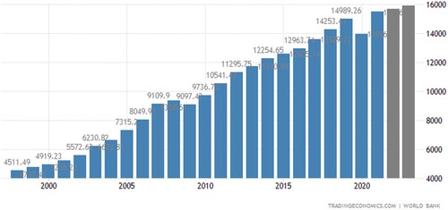
Georgia seceded from the former USSR in April 1991 and subsequently experienced civil war and economic turmoil. As mentioned above, GDP in Georgia collapsed by 80% and began to recover in 1996. The Rose Revolution of 2003 marked a watershed: corruption was stamped out, public order and democracy restored, free-market reforms implemented, and economic stability achieved (Jones 2013). Economic growth has been impressive and sustained (Figure 1). The war with Russia over South Ossetia (August 2008) reduced economic growth in 2008 and 2009, but it recovered subsequently. GDP per capita in 2019 was almost 20.5 times larger than at the time of the Rose Revolution (annual growth rate of 5.6%), and 3.5 times larger than in 1997 (annual growth rate of 5.8%).

Figure 1. Gross domestic product (GDP) per head, 1998–2022 (purchasing power parity (PPP)-adjusted US dollars at 2017 prices).

Source: Trading Economics based on World Bank data.

A graph showing that GDP per head grew at an annual average rate of 5.4% during 1998–2022.

Critics have questioned the sustainability of this success story on the grounds that economic growth has been consumer-led, and that although mass corruption has been stamped out, rent-seeking by business elites continues to take place, while the rule of law is honoured in the breach, especially with regard to property rights (Papava 2013, 2014). On the other hand, the economic recovery post COVID-19, testifies to the continued resilience of the Georgian economy (Figure 1) despite the failure to negotiate a free trade treaty with the European Union.

Labour and capital

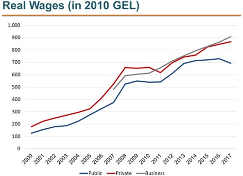
Real wages have grown alongside the growth in the economy (Figure 2). In the private sector real wages grew by 9% per year during 2000–17, whereas in the public sector real wages grew by 10% per year. Indeed, wages grew faster than GDP per capita.

Figure 2. Real wages, 2000–17 (lari at 2010 prices).

Source: Author’s calculation using GeoStat data.

A graph showing that during 2000–17 real wages grew in line with GDP per head, and that public sector pay lagged behind pay in the business and private sectors.

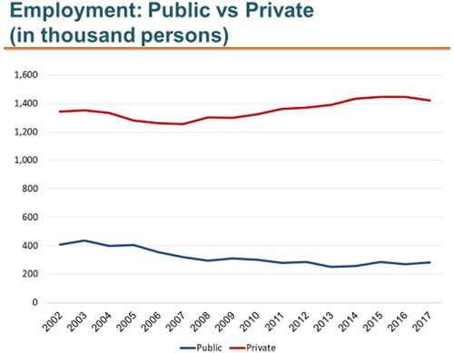
On the other hand, Georgia experienced negative demographics. The population as a whole contracted until 2013 (Figure 3) due to emigration, lower fertility and higher mortality, but has stabilized subsequently, although the population of working age contracted by slightly less. Nevertheless, the labour force remained flat thanks to an offsetting increase in participation in the labour force. The participation ratios in the rural and urban sectors have a similar pattern except for the fact that the rural participation ratio exceeded its urban counterpart by about 17 percentage points. This constellation of events is reflected in employment (Figure 4). Total employment remained flat; private employment grew at the expense of employment in the public sector.

Figure 3. Population, population of working age and employment, 1998–2017 (thousands).

Source: Author’s calculation using GeoStat data.

A graph showing that during 1998–2017 although Georgia experienced negative demographics, the population of working age and the labour force remained flat.

Figure 4. Employment in the public and private sectors, 2002–17 (thousands).

Source: Author’s calculation using GeoStat data.

A graph showing that during 2002–17 the public sector shed labour, which enabled employment growth in the private sector.

These negative demographics might have been expected to enhance rural–urban migration to satisfy labour shortages in the urban sector. The fact that this did not happen makes the absence of rural–urban migration all the more remarkable. On the other hand, these negative demographics explain why urban workers succeeded in capturing the benefits of GDP growth; the demand for labour grew faster than supply. Had the rural sector served as a reservoir for urban labour, urban wage growth would most probably have been less impressive.

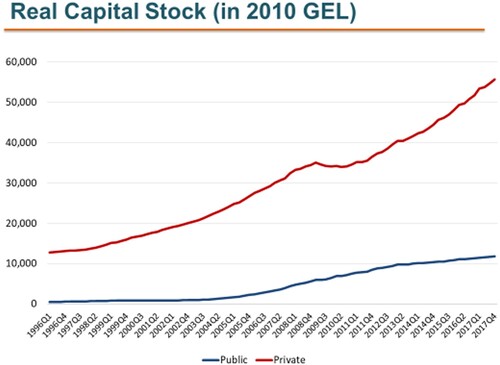
Capital investment has been rapid too. The private and public capital stocks have grown by fourfold (Figure 5). Since employment has been flat, Figure 5 implies that capital per worker increased fourfold, which explains the growth in wages reported in Figure 2. Therefore, economic growth has mainly been driven by the accumulation of capital; there has been no shortage of jobs.

Figure 5. Capital stock in the public and private sectors, 1996 quarter 1–2017 quarter 4 (lari at 2010 prices).

Source: Author’s calculation using GeoStat data.

A graph showing that during 1996–2017 the capital stock grew faster than the economy.

Urbanization

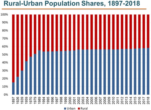
Substantial rural–urban transition occurred during the twentieth century until the fall of the USSR (Figure 6). Indeed, the urban population share increased from 15% at the end of the nineteenth century to 55% in 1989. Subsequently, however, the urban population share has scarcely increased, reaching 59% in 2021. In terms of the Lewis model, a large reservoir of rural population should have served as a source of labour to drive urban economic development. However, there is no evidence of the scale of rural–urban transition that might be expected in an economy in which real wages grew so rapidly.

Figure 6. Rural and urban population shares, 1897–2018 (%).

Source: Author’s calculation using GeoStat data.

A graph showing that since 1897 the urban population share grew at the expense of the rural population before the Revolution under the Soviet Union. Subsequently the urban population share has stabilized.

The rural sectors’ contribution to GDP is much smaller than its population share. On the other hand, the rural sectors’ contribution to self-employment greatly exceeds its population share. Self-employment accounted for 80% of rural employment in 1988. By 2017, it accounted for about 60%. This means that the wages reported in Figure 2 are largely urban, and that rural incomes largely accrue to smallholders, who are largely self-employed.

In summary, the rural population predominantly consists of smallholders while the urban population consists of salaried workers. Rapid wage growth has primarily benefited the urban population. However, the rural population has mainly stayed put.

Rural–urban wage differential

Since the late 1990s, the Statistical Office of Georgia (GeoStat) has conducted a household income and expenditure surveys known by ‘Shinda’, which consists of a rotating panel over four quarters of a stratified random sample of households. These data have been used by GeoStat to estimate average rural and urban incomes. An important feature of Shinda is the inclusion of home production as income. Home production largely refers to rural smallholders, who grow agricultural products on their homesteads. For example, if smallholder production of potatoes is sold on the market, their value added is included in market income. If instead, the potatoes are consumed by the smallholders, the value of home consumption based on the price of potatoes on the local market is included in their income. Home consumption includes dairy products, eggs, meat, fruits and vegetables, honey, firewood, etc. Shinda also includes home production in the urban sector, where it is much less important than in the rural sector. In short, Shinda is designed in the spirit of ‘normative informality’ in the sense of Fehlings and Karrar (2020).

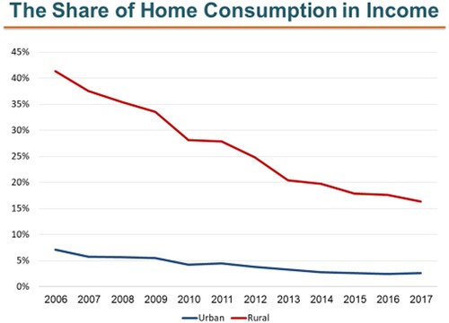
The share of home consumption in rural incomes is large but has been falling over time. Between 2002 and 2017 the rural share has fallen from 56% to 16% (Figure 7). Had home consumption been ignored, rural incomes would have been greatly under-reported relative to urban incomes. This bias would have been considerably smaller in 2017 but is still large. In summary, accounting for home consumption makes a large difference to the measurement of rural–urban income gaps. The same observation has been made by Iashvili (2020) who showed that during 2015–18 the rural–urban income gap disappears when non-cash income and transfers are included.

Figure 7. Share of home consumption in income in the rural and urban sectors, 2006–17 (%).

Source: Author’s calculation using GeoStat data.

A graph showing that during 2006–17 home consumption of homestead production constituted a large share of incomes in Georgia, especially in the rural sector. However, its importance has been decreasing.

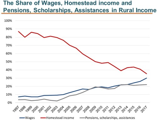
Figures 8 and 9 provide details about the composition of urban and rural incomes. In the rural sector, the share of wages in incomes increased from 9% in 2002 to 30% in 2017. The combined shares from self-employment, sales of agricultural produce and home production fell from 81.1% to 35.5% over the same period, and the share of transfers increased from 2.9% to 22.2%. The wage share in the urban sector increased from 33% to 47% over the same period, and the share of transfers increased from 18%. Figure 10 establishes that these trends were present before 2002. Indeed, in 1997 almost 90% of rural incomes were from self-employment. It also shows that following the Rose Revolution in 2003 government transfers became an increasingly important component of rural incomes (and urban incomes), accounting for 22% of rural incomes by 2017. In summary, rural incomes have become more diversified, more wage based, and more dependent on government transfers.

Figure 8. Composition of urban incomes, 2002–17 (lari).

Source: Author’s calculation based in Shinda (GeoStat).

A graph showing that during 2002–27 urban incomes became increasingly diversified. Transfer payments and income from property disposal have grown in importance. Remittances have remained stable and of limited importance.

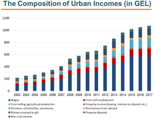
Figure 9. Composition of rural incomes, 2002–17 (lari).

Source: Author’s calculation using Shinda (GeoStat).

A graph showing that during 2002–07 rural income sources became more diversified than their urban counterparts. Transfer payments have been increasingly important, while home production continues to be large despite its declining importance.

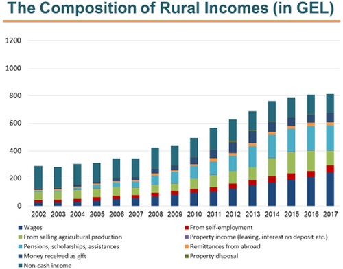
Figure 10. Shares of wages, homestead income and transfer payments in rural incomes, 1997–2017 (%).

Source: Author’s calculation.

A graph showing that during 1997–2017 rural income sources became more diversified than their urban counterparts. Transfer payments have been increasingly important, while home production continues to be large despite its declining importance.

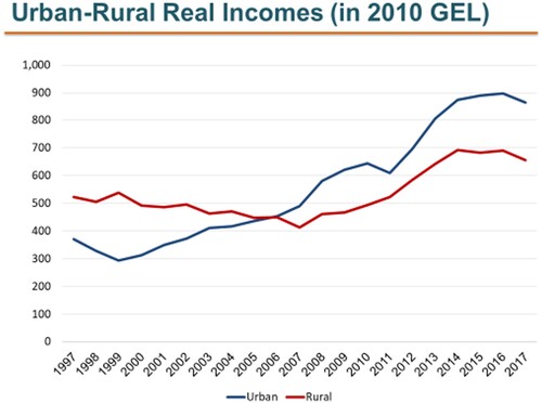
Figure 11 plots rural and urban standardized (for household composition) incomes in Figures 8 and 9 at constant (consumer price index – CPI) prices. It shows that urban incomes were initially lower than rural incomes, but have grown more rapidly than rural incomes. Rural incomes decreased until 2007, but have increased subsequently. Whereas the rural–urban income gap initially favoured the rural sector, matters changed in 2006 when urban incomes overtook rural incomes. The urban income gap has been increasing, as predicted by the Lewis model, but this has failed to induce rural–urban migration.

Figure 11. Average income in the rural and urban sectors, 1997–2017 (lari at 2010 prices).

Source: Author’s calculation using GeoStat data.

A graph showing that during 1997–2017 urban incomes were initially smaller than rural incomes. However, urban incomes eclipsed rural incomes in 2006, whence the urban–rural income gap has been widening.

Rural and urban costs-of-living

The data in Figure 11 ignore COL differences between the urban and rural sectors; they implicitly assume that COLs are the same in the rural and urban sectors. Even in advanced countries there are no subnational data for COLs. Some countries, including Georgia, have data on local CPIs, however, index data are not informative about absolute living costs. As far as rural and urban COLs in developing countries are concerned, the literature has been silent since Ravallion and van der Walle (1991) estimated rural and urban COLs for Java in 1981 based on housing costs and rice prices. By contrast, we calculate rural and urban COLs annually for Georgia, and cover all items of consumption including housing, durables and non-durables.

To fix the idea, suppose that there are two goods, A and B, which have different prices in rural and urban areas. Suppose further that the shares of these goods in rural and urban consumption baskets happen to be identical. In this case, the rural and urban COLs are comparable. Matters are different if the shares are not the same. If A and B are more expensive in urban areas than in rural areas, and A is more expensive than B, the rural COL may exceed the urban COL if the rural weight for A exceeds its urban counterpart. This does not mean that the comparison is invidious. If people migrate from the countryside to the towns, and adopt urban consumption patterns, they will experience the lower urban COL. The same would apply if people migrated from the towns to the countryside, where they adopted rural life styles. Under assimilation, urban and rural COLs are comparable even if rural and urban weights differ.

If migrants do not assimilate, it would be necessary to calculate urban COLs using rural weights instead of urban weights, and rural COLs using urban weights instead of rural weights. Since the relative price of A and B is expected to influence their weights in consumption, some assimilation is expected of migrants. Further assimilation is likely to occur as migrants copy incumbents more generally. COLs vary over time either because the prices of A and B change, and/or their weights change. Since A is more expensive than B, COLs will increase if more A is consumed, even if prices remain unchanged.

COL is made up of four main components: traded goods, non-traded goods and services, and housing. Traded goods mainly comprise consumer durables such as vehicles, furniture and electronic products whose wholesale prices, to a first approximation, are the same or similar everywhere. Non-traded goods and services include products such as fresh dairy products and vegetables, which are produced locally, and services such as hair-dressing and repairs. The housing component is universally problematic if households are owner–occupiers because their outlay on housing is zero. Matters are different if they are not owner–occupiers because they pay rent. Ideally, owner–occupiers should report the user cost of their housing, which is the value of their dwelling multiplied by the rate of interest plus the rate of depreciation, but they do not report this.

We use data from Shinda to construct rural and urban COLs. Urban COLs are expected to exceed rural COLs for a variety of reasons. The most important of these concerns the price of housing, which is expected to be smaller in the countryside. Shinda households in rented accommodation are asked to report their rent. If they are owner–occupiers, they are asked to assess their imputed rent. However, the response rate is low (21.2%). There is only a handful of rural households who reported that they pay rent. The vast majority are owner–occupiers who live in homesteads handed down from one generation to the next. Matters are only slightly better among urban households where, according to Shinda, 11.1% are living in rented accommodation. Another source of data is a panel of about 40 households living in rented accommodation used by GeoStat to calculate CPI’s for seven cities. We have constructed urban rents by averaging these data together with the imputed rents from Shinda. These two data sources have similar trends. By Western standards rents in Georgia are low both absolutely and relative to consumption in general. Rents account for only 10% of urban household consumption.

Since the collapse of the USSR urban housing markets have developed in Georgia, and especially in Tbilisi, the capital. According to Shinda, house prices in Tbilisi have more than doubled in real terms since 2002. In 2018 standardized housing cost about GEL100,000 (US$57,000 at 2010 exchange rates), and rents, which have followed the upward trend in house prices, were about GEL500 per month (US$285). Our estimate of urban rents is consistent with these data.

In the countryside, housing markets are less developed than in the cities. Public Registry data indicate that during 2010–17 there were about 600,000 urban property transactions and only 100,000 rural property transactions. The latter include an unknown number of inherited homesteads, which should be excluded. Since the numbers of rural and urban households are similar, these data suggest that turnover of property in the rural sector is a fraction of its urban counterpart. These differences might simply be induced by greater geographical mobility in the urban sector. However, they might be induced by thinness and illiquidity in the rural property market. According to Shinda only nine rural households during 2010–16 reported selling property, whereas 37 urban households reported selling property, and 21 rural households and 32 urban households bought property. Although Shinda does not identify the location of these properties, these data further suggest that the rural property market is less active than its urban counterpart. Finally, during 2015–18 only 1.2% of 151,303 dwellings offered for sale on websites referred to rural dwellings. Georgians are reluctant to sell their ‘family homes’ in the countryside. Most urban Georgians, including third generations, continue to feel attachment to their village of origin and their family homestead. Unlike the urban housing market, the rural housing markets should be understood in ethnographic terms. Under Georgian law, real estate including rural homesteads cannot be sold to foreigners.

This cultural phenomenon, which might not be unique to Georgia, means that the opportunity cost of rural housing is much smaller than for urban housing. Would-be migrants in the countryside cannot sell their homesteads or find it difficult to do so, but if they migrate to the urban sector, they would have to pay for their housing. Therefore, we assume that the weight of housing in the rural cost of living index is a fraction of its nominal value.

We construct geometrically weighted COL indices for the urban and rural sectors using price data and consumption shares for the types of goods as defined in Shinda. The first refers to the consumption of ‘everyday’ goods and services, such as food. The second refers to ‘intermittent’ goods and services, such as durables, but it also includes gas and electricity, which are billed intermittently. The third refers to rent (housing). Price and expenditure data for the first two categories are averaged across households in both sectors. We have assumed that the prices of gas and electricity are the same in the rural and urban sectors, and that the shares of gas and electricity in the second component are the same nationally (Mzhanvadze 2019).

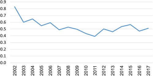
Figure 12 plots COL in the rural sector as a percentage of COL in the urban sector, which in 2002 was about 82%. Subsequently, the rural COL decreased relative to the urban COL, so that by 2011 the rural COL was only 40% of the urban. It suggests that the relative COLs have stabilized more recently, and the urban COL is twice its rural counterpart. The majority of the increase in the urban cost of living relative to its rural counterpart resulted from housing, which became more expensive in the towns relative to the countryside.

Figure 12. Cost-of-living in the rural sector relative to the cost-of-living in the urban sector, 2002–17.

Source: Author’s calculation using GeoStat data.

A graph showing that in 2002 the urban cost-of-living was only 20 higher than the cost-of-living in the rural sector. However, since 2008 the urban cost-of-living has been twice the rural cost-of-living.

Figure 13 adjusts Figure 11 for rural and urban living costs. The blue (urban) schedules in Figures 11 and 12 are identical. The red (rural) schedule in Figure 13 is obtained by dividing the red schedule in Figure 11 by the schedule in Figure 12. Whereas in Figure 11 urban incomes exceeded rural incomes after 2006, in Figure 13 rural COL-adjusted incomes always exceed urban incomes. Indeed, the percentage gap increases over time in favour of the rural sector.

Figure 13. Rural and urban incomes adjusted for the relative cost-of-living, 2002–17.

Source: Author’s calculation.

A graph showing that when the cost-of-living is taken into consideration, rural incomes exceed urban incomes in contrast to the opposite impression created by Figure 11.

We do not know why urban housing became more expensive for we have no estimates for Georgia of the income and price elasticities of demand for housing. Nor are there data on housing supply. Nevertheless, urban housing did not become more expensive because of demographic pressure due to rural–urban migration or population growth. This suggests that urban demand for housing space grew because of urban income growth, and that urban housing supply did not keep pace with the growth in demand.

We have decomposed the rural–urban cost of living differential in Figure 12 into its three price components: housing, daily goods and services and intermittent goods (durables and traded goods). This decomposition shows that the data in Figure 12 are dominated by housing costs. Had urban housing not become increasingly expensive relative to rural housing, the relative cost of living in Figure 12 would have remained at about 0.8 until 2012, increasing to 1 by 2017. This means that after 2006 COL-adjusted urban incomes would have exceeded rural incomes, and by 2017 COL-adjusted urban incomes would have exceeded rural incomes by 33% instead of being 35% smaller in practice. The fact that COL-adjusted rural incomes exceeded urban incomes was attributable to the increase in the relative cost of urban housing as well as the increasing share of housing costs in the urban COL.

Rural wage income

The share of wages in rural incomes has grown significantly (Figure 9), and the share of home consumption has declined (Figure 10). However, the proportion of rural households with no wage income has remained steady at about 60%. Therefore, the growth in the rural wage share did not happen because the rural population is increasingly abandoning the homestead in favour of full-time participation in the labour market. Instead, rural households have been increasingly diversifying their sources of income through wage employment.

Unfortunately, Shinda is silent on the sources of rural wages. If their source is from urban employment due to commuting to the towns, this would be tantamount to rural–urban migration. Matters would be different if the sources were from rural employment. Agricultural wage employment remained static during the early 2000s. After 2008 agricultural employment grew rapidly (by 300% by 2017), which is consistent with the argument that rural households increasingly found work in the rural sector, rather than by commuting to the towns. In any case, the cost of commuting in time and money would have deterred commuting to the towns.

Rural and urban unemployment

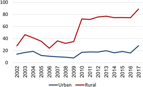
The COL-adjusted rural–urban income differential should be weighted by the probability of finding employment in the rural and urban sectors (Harris and Todaro 1970). If these probabilities are measured by 1 minus the rate of unemployment, the positive difference between COL-adjusted rural and urban incomes in Figure 13 would be even greater because urban unemployment rates exceed their rural counterparts in Georgia (Figure 14).

Figure 14. Unemployment rates in the urban and rural sectors, 2005–17 (%).

Author’s calculation based on GeoStat data.

A graph showing that during 2005–17 urban unemployment rates greatly exceeded rural rates of unemployment.

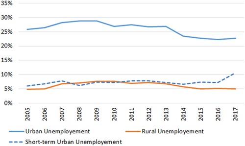
Figure 14 distinguishes between short-term urban unemployment up to 12 months’ duration and the overall rate of unemployment. The difference is accounted for by long-term unemployment. Since the unemployed in Georgia do not receive unemployment benefit, the long-term unemployed report that they have been actively seeking employment for more than a year, and even for more than three years. Because the urban short-term unemployment rate is broadly similar to the rural unemployment rate, excluding the urban long-term unemployed from the calculation of rural – urban income differentials, suggests that the results in Figure 13 are conservative.

Discussion

Georgia

There are a number of loose ends to the case study for Georgia. First, it is not clear how the national statistical office (GeoStat) took account in its national income accounting of informal output especially in the rural sector. According to Figure 10 this output accounted for 80% of rural incomes in 1997, but fell towards 30%. A related loose end is that although we have concentrated on urban economic growth, relatively little attention has been paid to the sources of rural economic growth. According to Figure 13, rural income grew at an average annual rate of 10.6% during 2002–17, while urban income grew at an annual rate of 11.2%. These growth rates, which include informal income, considerably exceed their standard counterparts in Table 1 and Figure 1. In short, the omission of informal income understates the rate of economic growth. A third, related loose end concerns the factors, which contributed to the growth in informal income, which are not studied here. A suggestion is that there was positive feedback from urban economic growth onto rural economic growth. Development theory tends to see the modern or urban sector as engine of economic growth. By contrast, the subsistence or rural sector is seen to be passive and backward (or slothful and indolent as Marx and Engels might have put it). The Georgian experience suggests a more nuanced model in which rural economic growth is an engine of growth in its own right.

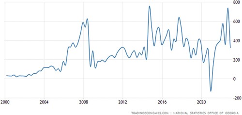
A quite separate loose-end concerns the factors, which contributed to the accumulation of capital (Figure 5), that are also not studied here, but which was the main driver of economic growth. Foreign direct investment has remained steady (Figure 15). Throughout the study period the rate of return on capital was large and exceeded the cost of capital, so the incentive to invest in fixed assets remained positive. To resolve this loose end it will be necessary to explain why the rate of return on capital did not decrease despite the increase in the capital stock.

Figure 15. Foreign direct investment, 2000–22 (US dollars millions).

Source: Trading Economics.

A graph showing that during 2000–22 foreign direct investment (FDI) accounts for much of gross domestic fixed capital formation. FDI was buoyant until the war with Russia in 2008. Since 2015 its former buoyancy has recovered.

On the other hand, the main issue has been resolved. We have explained how Georgia’s impressive economic development took place without substantial rural–urban migration. It remains to be seen whether this explanation is relevant to other CASC economies, especially Armenia.

Rural–urban fertility differentials

It is well established that rural fertility exceeds urban fertility in developing countries (Lerch 2019). In the absence of rural–urban migration this implies that the urban population share should decrease over time (assuming common mortality rates), in which event estimates of urbanization based on population shares are biased downwards. Indeed, flat rates of urbanization may be consistent with substantial rural–urban migration. If rural fertility in Georgia exceeds urban fertility the fact that the rural and urban population shares remained stable (Figure 6) might conceal substantial rural–urban migration.

Denoting the rural and urban fertility rates by m and n, it can be shown that the rate of rural–urban migration, which leaves the urban population share (π) unchanged, equals (m – n)/2.1π. For example, if rural fertility is 3 and urban fertility is 2.5, the rate of rural–urban migration must be 47% per generation (about 1.5% per year) if the rate or urbanization is to remain at 50%. This rate of rural–urban migration varies directly with the differential rate of fertility and inversely with the rate of urbanization. Buckley (1998) reports that in Central Asia rural fertility greatly exceeded urban fertility in 1980.

Unfortunately, data are not available for rural and urban fertility rates in Georgia. According to the World Bank, total fertility in Georgia has remained slightly below replacement since 1990, which together with emigration accounts for Georgia’s negative demographics. According to the State Statistics Committee in neighbouring Azerbaijan, urban fertility was 1.6 in 2000 and 2020, rural fertility decreased from 2.2 to 1.8 and national fertility decreased from 2.0 to 1.7. In Armenia, according to the Demographic Health Survey of the National Statistical Office, in 2015–16 rural fertility was 1.8 and urban fertility was 1.7. According to Baramidze (2021) ‘fertility rates in Georgia in rural areas are still higher than in urban areas, although there is a tendency for the two rates to become similar.’

The narrowing of the differential between rural and urban fertility is most probably related to fertility transition (Spoorenberg 2017) according to which the decrease in rural fertility lags behind the decrease in urban fertility. Consequently, the gap between rural and urban rates of fertility widens during the transition, but disappears once the transition is completed.

These admittedly rough data suggest that during the study period stability in the urban population share most probably did not conceal large-scale rural–urban migration in Georgia.

Policy implications

The failure of the Lewis model in Georgia may be attributed to the increase in the urban COL induced by economic development, and especially the cost of housing. The pace of economic development increased the demand for housing relative to its supply so that urban house prices increased. Had the supply of urban housing been more elastic and therefore more responsive to the demand for housing, rural–urban migration would have been more substantial in Georgia. Had the supply of housing been perfectly elastic, as implicit in the Lewis model, economic development in Georgia would have been even more impressive, and the ‘rule’ that sustained economic development cannot occur without rural–urban transition would have been more evident.

Housing supply constitutes a bottleneck to regional economic development in high income countries, especially, but not only, in densely populated countries. Planning laws, zoning policy and related regulations inhibit the elasticity of housing supply. Therefore, the key policy issue concerns enhancement of the elasticity of supply of urban housing, especially in countries in which the supply of land for urban development is more available.

Finally, urbanization is not a necessary or sufficient condition for economic development. Policy makers do not have to agree with the quotations heading this paper.

Conclusions

Despite the industrialization policy of the former Soviet Union, the rural population share in Georgia was large when she achieved independence with the collapse of the USSR. The same was true of other newly independent states in the South Caucasus and Central Asia. Whereas in South East Asia, Latin America, Africa and elsewhere rural–urban migration played a central role in economic development, this did not happen in Georgia. The Lewis model of economic development, which predicts that urbanization is a necessary condition for economic development, does not appear to apply to Georgia. In summary, Georgia is an exception to the ‘rule’ embodied in the headline quotations to this paper.

The reasons for this exceptionality are the focus of the present study. Using detailed survey data on formal and informal household incomes, and by constructing COL indices for the rural and urban sectors, we show that real income differentials between the rural and urban sectors in Georgia were not sufficient to make migration from the countryside worthwhile. Indeed, incipient migration from the countryside exerted upward pressure on urban living costs in general and the cost of housing in particular. Moreover, rural income responded positively to the growth in urban income. Thus, did the rural population share remain large in Georgia.

Acknowledgements

I thank the three referees for their helpful comments, and Lasha Labadze and Giorgi Mzhavanadze for their involvement.

Disclosure statement

No potential conflict of interest was reported by the author.

Notes

1 Rural amenities include non-economic reasons for preferring rural living, e.g. fresh air and quiet. Urban amenities include the attraction of ‘bright city lights’ etc.

1 In literature too (Williams 1985), rural–urban transition became a setting for numerous novels, poems and plays.

2 For which Lewis was awarded the Nobel Prize in Economic Science in 1979.

3 Cited when Krugman won the Nobel Prize in Economic Science in 2008.

4 Elasticity here refers to the percentage change (b) in the demand for housing space when income increases by 1%.

5 Rural amenities include non-economic reasons for preferring rural living, for example, fresh air and quiet. Urban amenities include the attraction of ‘bright city lights’, etc.

Appendix

Suppose that rural and urban house prices differ, but the prices of other goods and services, denoted by p are the same. The urban population share is denoted by π and the total population is denoted by N, which is assumed to be fixed. The demand for urban housing space measured in square meters (H) is assumed to vary proportionately with the urban population, to vary directly with urban incomes (Y) with elasticity b, and to vary inversely with urban house prices per square meter (P) with elasticity -c: (1) $H=\pi N{Y}^b{P}^{-c}$(1)

The urban cost-of-living is a geometric weighted average of urban house prices and the prices of other goods and services $P^u{p}^{1-u}$, where u denotes the share of housing in the urban cost-of-living. The rural cost-of-living index is simply p because, as explained in the text, rural housing is ‘free’. The ratio of rural and urban incomes adjusted for the cost-of-living is: (2) $\delta ={\displaystyle \frac{Y}{Y_R}{\left({\displaystyle \frac{p}{P}}\right)}^u}$(2)

Finally, the urban population share varies directly with δ and the urban-rural differential in amenities¹ (a) through a logit model: (3) $\pi ={\displaystyle \frac{1}{1+\exp (-a-mln\delta )}}$(3)

Rural-urban migration is more sensitive to the urban-rural income differential the greater is m. If the income differential is zero (δ = 1), the urban population share would be (1 + e^-a)^-1, which equals a half when a = 0 and is less than a half if a is negative. If urban incomes exceed rural incomes (δ > 1), a finite number of rural inhabitants migrate to the towns. The number is finite because inhabitants differ by their attachment to the countryside, and by their preferences for urban amenities.

Equation (3) implies that the growth in the urban population share is: (4) ${\displaystyle \frac{d\pi }{\pi }=m(1-\pi )[m(dlnY-udlnP-dln{Y}_R+udlnp)+da]}$(4)

Urbanization, as measured by π, varies directly with the growth in the urban-rural income and amenity differentials and inversely with the growth in the rural cost-of living. Solving equation (1) for urban house prices, substituting the result into equation (4), then setting equation (4) to zero gives the rate of growth in the urban housing stock, which maintains a stable level of urbanization (π): (5) $dlnH=-{\displaystyle \frac{c}{m}da+\left({\displaystyle \frac{ub}{c}-1}\right)dlnY+{\displaystyle \frac{c}{u}(dln{Y}_R-dlnp)}}$(5)

If urban house prices grow slower than required by equation (5), urbanization increases because the urban cost-of -living grows less rapidly. If instead urban house prices grow faster, urbanization will decrease. Equation (5) states that if urban amenities grow relative to rural amenities, the required rate of growth in the urban housing stock decreases for otherwise the urban population would increase. The advantage of urban living remains the same because urban house prices increase to offset the increase in urban amenities. Equation (5) also states that urban income growth has an indeterminate effect on the required rate of growth in the urban housing stock. It will be negative if ub is less than c. Since u is a fraction, this condition is satisfied unless the income elasticity of demand for urban housing space (b) is very small relative to the price elasticity (c). Finally, equation (5) states that an increase in rural income growth adjusted for the rural cost-of-living increases the required rate of growth in urban housing for otherwise de-urbanization would occur.

Equation (1) implies that the log change in urban house prices is: (6) $dlnP=\left[{\displaystyle \frac{1}{\pi }d\pi +bdlnY-dlnH}\right]{\displaystyle \frac{1}{c}}$(6)

Urban house price growth varies directly with demand driven by growth in urban population and income, and it varies inversely with the rate of growth of the urban housing stock.

Substituting equation (6) into equations (5) implies that the urban population share remains stable when the rate of growth of the urban housing stock is: (7) $dlnH=\left(b-{\displaystyle \frac{c}{u}}\right)(dlnY-dln{Y}_R+rdln{P}_R)$(7)

which is equation (1) in the text.

References

- Asian Development Bank Institute. 2014. Connecting Central Asia with Economic Centers. Tokyo: ADBI.
- Baramidze, L. 2021. Reproductive Health in Georgia. Geneva: WHO.
- Beenstock, M., and D. Felsenstein. 2008. “Heterogeneity, Conditional Convergence and Regional Inequality.” Regional Studies 42: 475–488.
- Brakman, S., H. Garretsen, and C. Van Marrewijk. 2009. The New Introduction to Geographical Economics. 2nd ed. Cambridge University Press.
- Buckley, C. 1998. “Rural – Urban Differentials in Demographic Processes: The Central Asian States.” Population Research and Policy Review 17: 71–89. doi:10.1023/A:1005899920710.
- Capannelli, G., and R. Kanbur. 2019. Good Jobs for Inclusive Growth in Central Asia and the South Caucasus. Manila: Asian Development Bank.
- Chen, H., H. Zhang, W. Liu, and W. Zhang. 2014. “The Global Pattern of Urbanization and Economic Growth from the Last Three Decades.” PLOS One 9 (8): e103799. doi:10.1371/journal.pone.0103799.
- Combes, P.-P., T. Mayer, and J.-F. Thisse. 2008. Economic Geography: The Integration of Regions and Nations. Princeton, NJ: Princeton University Press.
- Engels, F. 1845. The Condition of the Working Class in England, 1974. St Albans: Panther.
- Fehlings, S., and H. H. Karrar. 2020. “Negotiating State and Society: The Normative Informal Economics of Central Asia and the Caucasus.” Central Asian Survey 39: 1–10. doi:10.1080/02634937.2020.1738345.
- Harris, J. R., and M. P. Todaro. 1970. “Migration, Unemployment and Development: A Two-Sector Model.” American Economic Review 60: 126–142.
- Henderson, J. V. 2010. “Cities and Development.” Journal of Regional Science 50: 515–540. doi:10.1111/j.1467-9787.2009.00636.x.
- Iashvili, T. 2020. “The Assessment of Income Inequality in Georgia: The Rural–Urban Disparity in Income.” Ekonomisti 3: 135.
- Jones, S. F. 2013. Georgia: A Political History Since Independence. London & New York: I. B. Tauris.
- Kelley, A. C., and J. G. Williamson. 1984. “Population Growth, Industrial Revolutions and the Urban Transition.” Population and Development Review 10: 419–441. doi:10.2307/1973513.
- Kelly, F. P. 2021. Migration, Agrarian Transition and Rural Change in South East Asia. London: Routledge.
- Krugman, P. 1991. Geography and Trade. MIT Press.
- Lerch, M. 2019. “Fertility Decline in Urban and Rural Areas of Developing Countries.” Population and Development Review 45: 301–320. doi:10.1111/padr.12220.
- Lewis, W. A. 1954. “Development with Unlimited Supplies of Labour.” Manchester School of Economics and Social Studies 22: 139–191. doi:10.1111/j.1467-9957.1954.tb00021.x.
- Marx, K., and F. Engels. 1848. The Manifesto of the Communist Party.
- Mzhanvadze, G. 2019. Estimating the Cost of Living in Rural and Urban Georgia. Mimeo ISET.
- OECD. 2018. Enhancing Competitiveness in Central Asia. Paris: OECD.
- Padawangi, R. 2022. Urban Development in South East Asia. Cambridge University Press.
- Papava, V. 2009. “Georgia’s Economy: Post-Revolutionary Development and Post-War Difficulties.” Central Asian Survey 28: 199–213. doi:10.1080/02634930903043717.
- Papava, V. 2013. “Economic Achievements of Post-Revolutionary Georgia: Myths and Reality.” Problems of Economic Transition 56: 51–65. doi:10.2753/PET1061-1991560204.
- Papava, V. 2014. “Georgia’s Economy: The Search for a Development Model.” Problems of Economic Transition 57: 83–94. doi:10.2753/PET1061-1991570304.
- Pomfret, R. 2019. The Central Asian Economies in the 21st Century: Paving a New Silk Road. Princeton, NJ: Princeton University Press.
- Pomfret, R. 2021. “Central Asian Economies: Thirty Years After the Dissolution of the Soviet Union.” Comparative Economic Studies 63: 537–556. doi:10.1057/s41294-021-00166-z.
- Ravallion, M., and D. van der Walle. 1991. “Urban–Rural Cost-of-Living Differentials in a Developing Economy.” Journal of Urban Economics 29: 113–127. doi:10.1016/0094-1190(91)90030-B.
- Ravenstein, E. J. 1885. “The Laws of Migration.” Journal of the Royal Statistical Society 48: 167–227.
- Ravenstein, E. J. 1889. “The Laws of migration.” Journal of the Royal Statistical Society 52: 214–301. doi:10.2307/2979333.
- Redford, A. 1924. Labor Migration in England 1800–1850, 1968. Edited and revised by W. H. Chaloner. New York: Augustus Kelley.
- Restrepo Cadavid, P., G. Cineas, L. E. Quintero, and S. Zhukova. 2017. Cities in Eastern Europe and Central Asia: A Story of Urban Growth and Decline. Washington, DC: The World Bank.
- Roback, J. 1982. “Wages, Rents and the Quality of Life.” Journal of Political Economy 90: 1257–1278. doi:10.1086/261120.
- Spoorenberg, T. 2017. “The Onset of Fertility Transition in Central Asia.” Population 72: 473–504. doi:10.3917/popu.1703.0491.
- Williams, R. 1985. The Country and the City. London: Hogarth Press.
- World Bank, 2009. World Development Report: Reshaping Economic Geography. Washington, DC: The World Bank.
- Yormirzoev, M. 2022. “Economic Growth and Productivity Performance in Central Asia.” Comparative Economic Studies 64: 520–539. doi:10.1057/s41294-021-00156-1.