Numerical and experimental investigations of human swimming motions

ABSTRACT

This paper reviews unsteady flow conditions in human swimming and identifies the limitations and future potential of the current methods of analysing unsteady flow. The capability of computational fluid dynamics (CFD) has been extended from approaches assuming steady-state conditions to consideration of unsteady/transient conditions associated with the body motion of a swimmer. However, to predict hydrodynamic forces and the swimmer’s potential speeds accurately, more robust and efficient numerical methods are necessary, coupled with validation procedures, requiring detailed experimental data reflecting local flow. Experimental data obtained by particle image velocimetry (PIV) in this area are limited, because at present observations are restricted to a two-dimensional 1.0 m² area, though this could be improved if the output range of the associated laser sheet increased. Simulations of human swimming are expected to improve competitive swimming, and our review has identified two important advances relating to understanding the flow conditions affecting performance in front crawl swimming: one is a mechanism for generating unsteady fluid forces, and the other is a theory relating to increased speed and efficiency.

KEYWORDS:

• Computational fluid dynamics
• particle image velocimetry
• robot
• swimming simulation model
• pressure distribution
• unsteady fluid force

1. Introduction

Today, success in the field of competitive swimming requires that swimmers and coaches have an understanding of fluid dynamics. This is highly challenging as the subject area is extremely complex, addressing multidisciplinary problems with a broad spectrum of research approaches (Wei, Mark, & Hutchison, 2014). To enable a better understanding of the fluid dynamics of human swimming, Wei et al. (2014) reviewed the existing research articles concerned with the fluid-dynamics-related aspects of swimming over the past five decades, and provided suggestions for improving performance; however, their study did not address the most up-to-date research in this area.

The field of computational fluid dynamics (CFD) is constantly advancing, and has been increasing our understanding of complicated hydrodynamic phenomena over several decades. In addition, particle image velocimetry (PIV) has proven to be a powerful tool for measuring actual flow fields around swimmers. Combining the results from CFD and PIV should help us considerably in visualising and understanding complicated hydrodynamic mechanisms. Moreover, actual experimental data, such as measurements of the relevant forces and pressures, are valuable to verifying CFD results, and as an aid to the interpretation of PIV images. Several experiments (Kudo, Yanai, Wilson, Takagi, & Vennell, 2008; Nakashima & Takahashi, 2007; Takagi & Wilson, 1999) have been performed to measure unsteady fluid forces or pressures on a mechanical arm, a swimming robot and human swimmers via the attachment of pressure sensors. Nakashima (2006) has developed a simulation model that uses parameters derived from such experimental data, for example moving velocity and fluid forces; the model is called the swimming human simulation model (SWUM). If we can combine novel and sophisticated methodologies such as CFD, PIV and SWUM, then we may be able to uncover the complex mechanisms that generate unsteady fluid forces while swimming.

It has been only about 15 years since these methodologies have come into practical use in human swimming research; notably, little information is available concerning the inherent limitations and potential of these methodologies. This paper reviews the numerical and experimental investigations of swimming from the start of these investigations to the present time, and discusses an appropriate methodology to resolve persistent problems still remaining in this area.

The review was conducted in accordance with the ethics guidelines expressed in the Declaration of Helsinki.

2. Computational fluid dynamics (CFD)

CFD is a numerical simulation technique for solving the Navier–Stokes equations of fluid flow (Ferziger & Perić, 2012). Because the equations are non-linear, in both space and time, they are solved using numerical discretisation techniques. For the space discretisation, the computational domain is divided into a large number of individual cells or meshes, on which the velocities and pressures are defined. To resolve turbulent flow directly with such a mesh, the cell size must be smaller than the minimum vortex length, the so-called Kolmogorov length scale η, defined as:

(1)

where ν is the kinematic viscosity of water, L a reference length and U a typical forward speed (Rogallo & Moin, 1984). For the flow around a swimmer, η is of the order of 2.0 μm, assuming typical values ν = 10⁻⁶ m²· s⁻¹, L = 2 m and U = 2 m· s^–1. Here, ν is based on the order of the kinematic viscosity of water in a swimming pool, and the values L and U are the order of a typical world-class swimmer’s height and advancing speed, respectively. If cubic-shaped cells are employed for the computational domain, this means that each side must be of length not exceeding 2.0 μm, for a domain of relevance; say 2 m × 2 m × 4 m, the total number of cells would be 2 × 10¹⁵ (i.e. 2000 trillion). Even in an age of petaflop computer technology, a transient simulation featuring this number of meshes is unfeasible. Thus, to make progress, turbulence models need to be employed, in which turbulent phenomena are modelled, not calculated explicitly. Unfortunately, there is no universal turbulence model known that can be applied to all types of flows, though reliable, approximate models do exist for specific cases (Kleinstreuer, 1997). Consequently, CFD simulations involving the use of turbulence models will incur errors. As well as the physical modelling errors, any CFD simulation will involve numerical errors resulting from the finite resolution, if sufficiently fine mesh is not possible to resolve all the macroscopic scales of relevance. Thus, a grid-dependence study (Roach, 1998) is mandatory to achieve reliable quantitative numerical predictions.

The first studies using CFD were undertaken at the Los Alamos National Labs in the 1950s in the context of the development of airfoils; these works have been reviewed by Harlow (2004). In accordance with the improvements in numerical algorithms and computer capabilities, two-dimensional (2D) simulations were eventually extended to three dimensions, and today flows around complex geometries can include additional physical phenomena, such as two-phase or multi-phase flow conditions (e.g. bubbly flow), phase change (e.g. boiling flow), fluid–structure interaction (e.g. blood flow through flexible arteries). CFD simulations for swimmers resemble in many respects those for ships: a body advances close to, or just under, the water surface, subject to a balance of drag and thrust forces. Nonetheless, compared with CFD simulations applied to ships (Stern, Yang, Wang, Sadat-Hosseini, & Mousaviraad, 2013), the difficulties of simulating a human swimming lie in the treatment of (i) the complicated and transient movements of a flexible body shape in the water; (ii) the dynamically changing shape, with rotations of many body segments about multiple axes not aligned with the orthogonal external reference system or direction of travel; and (iii) the large deformation of the water surface relative to the size of the swimmer; such complications do not exist in the case of ships, and are challenging. Besides the difficulties associated with the CFD methodology itself, as outlined in the previous paragraphs, the validation of CFD simulations for swimmers is in itself not at all straightforward, due to the limitations in accurately measuring the flow around the swimmer.

CFD studies of human swimmers began with steady and accelerated flows around a 2D disc (Bixler & Schloder, 1996), the disc being a simplification of the swimmer’s hand. The commercial CFD code Fluent® was used for these simulations, using three different turbulence models: the standard k–ε model (Launder & Spalding, 1972); the re-normalisation group k–ε model (Orszag et al., 1993); and the Reynolds stress model (Gibson & Launder, 1978). These studies were undertaken in order to evaluate the influence of turbulence model on the hydrodynamic forces. The most accurate drag force was obtained by the Reynolds stress model. From comparisons of the calculated drag forces for quasi-steady (in order to simplify transient flows, the hydrodynamic forces exerted on a body moving unsteadily within a fluid are assumed to be determined at any instant only by the flow field at that instant) and accelerated flow conditions, the authors were able to demonstrate that the drag under accelerated conditions is larger than that for quasi-steady conditions by almost 40%, clearly indicating the need for performing simulations under transient conditions (i.e. in the accelerated flow condition) instead of adopting the quasi-steady assumption. Following this study, many CFD simulations (Alves, Marinho, Leal, Rouboa, & Silva, 2007; Bilinauskaite, Mantha, Rouboa, Ziliukas, & Silva, 2013; Bixler & Riewald, 2002; Gardano & Dabnichki, 2006; Marinho, Barbosa, Rouboa, & Silva, 2011; Marinho et al., 2009b, 2010; Minetti, Machtsiras, & Masters, 2009) were carried out for the flow around a hand and forearm under steady-state conditions (an object or a body is statically placed in a uniform flow without any body motion); these are listed in Table 1. Although these steady-state simulations are, in principle, capable of estimating the thrust and lift forces, results are limited, as exemplified by Bixler and Schloder (1996), because the swimmer’s stroke path is usually curved, and the hand is accelerating.

Table 1. Summary of CFD simulation for hand and arm in steady state condition.

Authors	Participants	Object	2D/3D	CFD code	Turbulence model*
Bixler and Schloder (1996)	Flow around flat plate	Flat plate	2D	Fluent®	k–ε, RNG and RSM
Bixler and Riewald (2002)	Flow around hand and forearm	Hand, forearm	3D	Fluent®	k–ε
Gardano and Dabnichki (2006)	Flow around arm	Arm	3D	Fluent®	N/A
Alves et al. (2007)	Flow around hand and forearm	Hand, forearm	3D	Fluent®	k–ε
Marinho et al. (2009b)	Flow around hand with different thumb positions	Hand	3D	Fluent®	k–ε
Minetti et al. (2009)	Optimum finger spacing	Hand	3D	CFX®	k–ε and k–ω
Marinho et al. (2010)	Flow around hand with small finger spread	Hand	3D	Fluent®	k–ε
Marinho et al. (2011)	Flow around hand and forearm	Hand, forearm	3D	Fluent®	k–ε
Bilinauskaite et al. (2013)	Quasi-steady approach for fluid forces of hand	Hand	3D	Fluent®	k–ε

*Turbulence model

k–ε, Standard k–ε; RNG, re-normalisation group k–ε; RSM, Reynolds stress model.

A steady-state simulation of the flow around a swimmer’s body in a prone, gliding position may be more appropriate than one of a hand only, because such a condition occurs in practice just after the start or the turn, in competitive swimming. Three-dimensional (3D) simulation of the flow around a gliding swimmer was first attempted by Lyttle and Keys (2004) using Fluent®. The body shape of an elite swimmer was scanned optically, and the surface of the swimmer represented by 60,000 triangular elements. Bixler, Pease, and Fairhurst (2007) later also simulated the flow around a swimmer in a prone gliding position. An experiment using a mannequin, whose shape is identical to that adopted for the CFD simulation, was undertaken in a water flume for the purposes of validation. The drag forces predicted by CFD agreed with measured data within an error bound of 4%, and revealed that, in the range of 1.5 ≤ U ≤ 2.25 m · s⁻¹, approximately 75% of the drag is due to pressure forces (i.e. form drag) and 25% due to friction. The computed total drag coefficient (C_d = D/0.5 ρ · U² · A, where A is the frontal projected area) was about 0.3. Following Bixler’s research, simulations of the flow around a gliding swimmer without body motion were performed by other groups (Machtsiras, 2012; Marinho et al., 2009a, 2011; Popa et al., 2011; Sato & Hino, 2010; Silva et al., 2008; Zaidi, Fohanno, Taiar, & Polidori, 2010; Zaidi, Taiar, Fohanno, & Polodori, 2008); these are summarised in Table 2.

Table 2. Summary of CFD simulation for full body in steady-state condition.

Authors	Participants	Object	2D/3D	CFD code	Turbulence model*
Lyttle and Keys (2004)	Flow around gliding swimmer	Full body	3D	Fluent®	N/A
Bixler et al. (2007)	Flow around gliding swimmer	Full body	3D	Fluent®	k–ε
Silva et al. (2008)	Two gliding swimmer in row	Full body	2D	Fluent®	k–ε
Zaïdi et al. (2008)	Gliding swimmer different head positions	Full body	2D	Fluent®	k–ε
Marinho et al. (2009a)	Flow around gliding swimmer	Full body	3D	Fluent®	k–ε
Sato and Hino (2010)	Flow around gliding swimmer near free surface	Full body	3D	SURF	SA
Zaïdi et al. (2010)	Flow around gliding swimmer	Full body	3D	Fluent®	k–ε and k–ω
Marinho et al. (2011)	Flow around gliding swimmer	Full body	2D	Fluent®	k–ε
Popa et al. (2011)	Flow on gliding swimmer with different head positions	Full body	3D	Fluent®	k–ω
Machtsiras (2012)	Flow around gliding swimmer with different head positions, gliding depths and swim suits	Full body	3D	Star-CCM+®	LES

*Turbulence model

k–ε, Standard k–ε; k–ω, standard k–ω; LES, Large-Eddy Simulation.

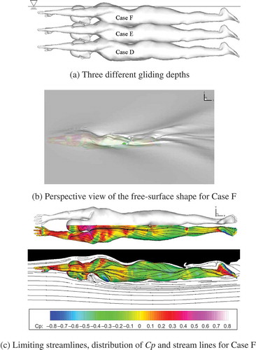
Sato and Hino (2010) performed simulations of the flow around a swimmer gliding at different depths using the Spalart–Allmaras turbulence model (Spalart & Allmaras, 1994) as shown Figure 1. Note that the Spalart−Allmaras model was originally developed for aerospace applications, but has also been applied to ship hydrodynamics through validation exercises (Larsson, Stern, & Visonneau, 2014). The wave-making resistance was predicted to contribute 20% to the total drag when the swimmer’s body was slightly below the water surface (Figure 1(b and c)). Zaidi et al. (2010) carried out CFD flow simulations around a swimmer using two turbulence models: the standard k–ε model and the standard k–ω model (Wilcox, 1988). Note that the standard k–ω model is more accurate in near wall treatment than the standard k–ε model, and is more suitable for separated flows. The total drag computed using the k–ε model was approximately 40% lower than experimental measurement (Bixler et al., 2007; Vennell, Pease, & Wilson, 2006), whereas the result of the k–ω model was in agreement within an error of 3% for the case of an advancing speed of 2 m · s⁻¹. More recently, Machtsiras (2012) has simulated the flow around a swimmer using the Large-Eddy Simulation approach (Smagorinsky, 1963). In Large-Eddy Simulation, large scales of turbulence are directly resolved, and only the small scales of turbulent motions are modelled. Compared with Reynolds-Averaged Navier-Stokes approach (i.e. simulations employing turbulence models such as the Spalart–Allmaras, k–ε or k–ω models, in which all the scale of turbulence is modelled), Large-Eddy Simulation is expected to be more accurate, though its application does require a finer computational mesh than that for the Reynolds-Averaged Navier-Stokes approach, implying higher computational cost. Results using Large-Eddy Simulation were of higher accuracy than those obtained using the k–ε model. In particular, the average drag obtained using Large-Eddy Simulation was less than 3% in error of that measured by Bixler et al. (2007), but was around 18% in error when the k–ε model was used.

Figure 1. Conditions of calculation and calculation results of a gliding swimmer for Case F. Three different gliding depths; Case D, 0.5 m; Case E, 0.3 m; and Case F, 0.1 m. As calculating conditions, Reynolds number was 2.9 × 10⁶, Froude number was 0.48 and advancing speed was 2.0 m · s^–1 (Sato & Hino, 2010). (a) Three different gliding depths; (b) perspective view of the free-surface shape for Case F; (c) limiting streamlines, distribution of Cp and stream lines for Case F.

Many CFD studies have been undertaken for flows around fixed bodies, since such simulations are relatively straightforward: that is, the treatment of the body motion is unnecessary, it representing just a fixed boundary to the flow. However, applied to a swimmer in motion, the continuous movement of the swimmer’s body must be taken into account as this is essential for accurately predicting the overall thrust and drag forces, as well as other aspects of swimming, such as stroke and kick simulations. Thus, the problem of analysing the flow of a swimmer with dynamically changing posture and limb orientations is an extremely complex and challenging one. In the CFD simulation method, there exist essentially three approaches for dealing with body motion: (i) a moving or dynamic grid approach including overset/overlapping grids (Hirt, Amsden, & Cook, 1974; Noack, 2005; Suhs, Rogers, & Dietz, 2002); (ii) a cut cell or immersed boundary approach (Mittal & Iaccarino, 2005); and (iii) a meshless approach (Monaghan, 2012).

The first attempt to use CFD to simulate the moving body of a swimmer (i.e. a swimmer with changing orientation and actively moving body segments) was made by Kawai (1997). The 2D flow around the swimmer, performing a dolphin kick, was computed using the cut cell method, as implemented in the commercial CFD code, STREAM®. Following this initial study, a variety of CFD simulations incorporating the moving body of the swimmer were performed (Cohen, Cleary, & Mason, 2012; Hochstein, Pacholak, Brücker, & Blickhan, 2012; Keys, 2010; Lecrivain, Slaouti, Payton, & Kennedy, 2008; Pacholak, Hochstein, Rudert, & Brücker, 2014; Rouboa, Silva, Leal, Rocha, & Alves, 2006; Sato & Hino, 2003, 2013; von Loebbecke & Mittal, 2012; von Loebbecke, Mittal, Fish, & Mark, 2009b; von Loebbecke, Mittal, Mark, & Hahn, 2009c). These are summarised in Table 3.

Table 3. Summary of CFD simulation for moving body.

Authors	Participants	Object	2D/3D	Treatment of motion	CFD code	Turbulence model*
Kawai (1997)	Dolphin kick	Leg and foot	2D	Cut cell	STREAM®
Sato and Hino (2003, 2010)	Stroke of swimmer	Hand	3D	Moving grid	SURF	Without
Rouboa et al. (2006)	Linear acceleration	Hand and forearm	3D	Body force	Fluent®	k–ε
Lecrivain et al. (2008)	Stroke of upper arm	Body and upper arm	3D	Dynamic mesh	Fluent®	N/A
von Loebbecke et al. (2009b, 2009c)	Dolphin kick	Full body	3D	IB	VICAR3D	Without
Keys (2010)	Dolphin, freestyle and breaststroke kick Freestyle swimming at water surface	Full body	3D		Fluent®	Realisable k–ε
von Loebbecke and Mittal (2012)	Stroke of swimmer	Hand and arm	3D	IB	VICAR3D	Without
Cohen et al. (2012)	Dolphin kick	Full body	3D	SPH	In-house	Without
Hochstein et al. (2012)	Dolphin kick	Full body	3D		OpenFOAM	N/A
Sato and Hino (2013)	Stroke of swimmer	Hand	3D	Moving grid	SURF	Without
Pacholak et al. (2014)	Dolphin kick	Full body	3D		OpenFOAM	N/A

*Turbulence model

k–ε: Standard k–ε.

In the von Loebbecke et al. (2009a, 2009b, 2009c) studies, the flow around a human body performing the dolphin kick motion was simulated. In these simulations, the swimmers were assumed to advance at a constant speed in water of infinite depth. The mean active drag for a female swimmer was estimated to be 135 N at a speed of 0.95 m · s^–1. The computed flow field for this female swimmer is shown in Figure 2, which clearly illustrates the vortices generated by the leg motion. From these studies, the authors concluded that most of the thrust was produced by the feet, the down kick producing a much larger thrust than the up kick. The propulsive efficiency of the dolphin kick was estimated to be within a relatively wide range: from 11% to 29% (von Loebbecke et al., 2009b). Hochstein et al. (2012) and Pacholak et al. (2014) also simulated the flow around an entire body performing the dolphin kick using the open source CFD code, OpenFOAM®. The formation and interaction of vortices near the swimmer’s body, and in the swimmer’s wake, were identified during successive dolphin kick cycles. These authors also demonstrated that maximum thrust was generated during the down kick, and that this was approximately twice that of the up kick. The predicted 3D vortex rings in the wake region are similar to those computed by von Loebbecke et al. (2009c).

Figure 2. Flow around a female swimmer advancing with dolphin kick. Topology of vortex structures (left), a slice containing flow vectors and flow speed contours (middle) and a slice containing vorticity contours (right) (von Loebbecke et al., 2009c).

A common problem of CFD simulations of swimmers, as discussed earlier, is that a quantitative validation procedure has not been performed, except in some isolated cases; for example, Bixler et al. (2007); Machtsiras (2012); and Sato and Hino (2013). Here, the quantitative validation procedure is ideally that: (i) an identical body shape is used in the experiment and the CFD simulation under the same boundary conditions; (ii) a grid-dependence study (Roache, 1998) is performed; (iii) the resolution of the flow-field measurement is high enough to evaluate the local velocity/pressure field, and thereby to validate the turbulence models; and (iv) both global quantities (e.g. the hydrodynamic forces acting on a body) and local quantities (e.g. velocity at a specific point) are compared between measurement and simulation. In the case of transient simulations incorporating body motion, validation becomes difficult because local velocity estimations are prone to error. However, local velocity can be measured experimentally using PIV. Further, forces and moments acting on body segments can be measured accurately with robotic bodies. Thus, the potential for improving the accuracy and effectiveness of the simulations by combining methods is apparent.

3. Particle image velocimetry (PIV)

PIV is an optical method for flow visualisation that can be used to measure instantaneous velocities and related properties, such as normal and shear stress, in fluids. An excellent review of the subject has been presented by Adrian (1991). PIV is the member of a broader class of measuring techniques to determine flow velocities in restricted regions of a fluid over time. Such methods estimate the local velocity (u) using the discretised equation:

(2)

where ∆x is the displacement of a marker originally located at position x at time t during a short time interval ∆t. The most up-to-date PIV setup consists of one or more high-speed CCD cameras (sampling at frequency above 200 Hz), a laser (Nd:YAG lasers are commonly used) controlled by an optical system, a synchronizer to act as an external trigger for the control of the CCD cameras and the laser, a marker or “seed particle” (usually with a diameter of the order of 10–100 μm and ideally with the density similar to that of the fluid) and the fluid under investigation.

PIV has been used successfully to study the locomotion of fish (Drucker & Lauder, 1999; Nagayama, Tanaka, Tanaka, Hayami, & Aramaki, 2008; Sakakibara, Nakagawa, & Yoshida, 2004), as well as insects (Dickinson, Lehmann, & Sane, 1999; Fearing et al., 2000). Matsuuchi et al. (2004) were the first to apply PIV to the research of swimming technique by measuring the flow field that develops around a moving hand while swimming, which may be the main source of propulsion for the crawl stroke. Sequential variations of the velocity field are shown in Figure 3. A remarkable amount of momentum generation was observed during the transition from insweep to upsweep motions during the latter part of the front crawl stroke (Figure 3(b)) because of the action of a pair of counter-rotating vortices. Matsuuchi et al. (2009) suggested that this increase in momentum directly leads to the unsteady fluid force generated according to Newton’s second law of motion. Subsequently, Matsuuchi and his group (Muramatsu, Matsuuchi, Nomura, Sakakibara, & Miwa, 2008; Yamada et al., 2006) developed a new PIV system combined with motion analysis. This system synchronises PIV images with 3D motion data by using two high-speed cameras to simultaneously capture the flow velocity fields for the geometrical configuration of the hand. The results obtained reveal that when the hand orientation was changed rapidly, vortex generation and shedding were observed, and thereby the momentum changes were detected in the flow field. Such vortex behaviour might contribute to the generation of thrust (Matsuuchi & Muramatsu, 2011). In addition to the front crawl, Kamata, Miwa, Matsuuchi, Shintani, and Nomura (2006) attempted to demonstrate the flow field during sculling movements and concluded that after the change in the direction of the hand motion, a pair of vortices formed with a jet flow induced between the vortices. This jet flow increased the momentum, and accordingly, a lift force exerted on the hand was believed to be generated. Takagi, Shimada et al. (2014) also performed a flow visualisation experiment during sculling using PIV and the measurement of the pressure distribution around a hand. A series of PIV images covering the period when the maximum resultant fluid force was produced is shown in Figure 4. Takagi, Shimada et al. (2014) concluded that a skilled swimmer produces large unsteady fluid forces during sculling when a leading-edge vortex occurs on the dorsal side of the hand and when wake capture occurs on the palm side (see Figure 4(II-b)). Beside the sculling movement, the PIV system has been extended to include the measurement of vortices during dolphin kicking (Hochstein & Blickhan, 2011; Miwa, Matsuuchi, Shintani, Kamata, & Nomura, 2006; Miwa et al., 2005). Hochstein and Blickhan (2011) found that vortices generated in the region of strongly flexing joints acted as a form of pedalling and enhanced propulsion, the so-called vortex re-capturing (Figure 5).

Figure 3. Sequential variations of the velocity field at 70 ms intervals ((a) → (b) → (c) → (d)) for a trained swimmer. The flume speed was set at 1.2 m · s^–1. The colour beside the velocity field represents the strength of the vorticity, measured in units of 1 s^–1. The five filled circles in (b) correspond to the fingers. The strongest vortex pair is visible in panel (b). The maximum and minimum vortices are 135.3 s^–1 (+) and −108.1 s^–1 (○), respectively (Matsuuchi et al., 2009).

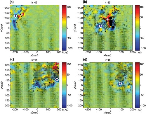
Figure 4. Still images of hand (column a), computer-generated maps of vorticity and velocity (column b) and pressure distribution around the hand (column c) at each of the four critical phases (rows I–IV) in sculling. The still images were recorded looking up from below the bottom of the controlled-flow water channel, and the hand is moving from a swimmer’s side towards the centre line of body. In the maps of vorticity and velocity, the colour bars at the right indicate the direction and strength of the vortex: red and blue indicate counterclockwise and clockwise, respectively, and colour intensity relates to vorticity strength. The small arrows indicate the velocity of the flow field. For the graphs of pressure distribution (column c), the horizontal axes indicate the sensor’s position normalised to the width of the hand (d). The vertical axes indicate the pressure values detected by each sensor (p1–p12). Sensors p2, p3, p4 and p5 were attached to the palm side of the fifth, fourth, third and second fingers, respectively. Sensors, p7, p8, p9 and p10 were attached to the dorsal side of the second, third, fourth and fifth fingers, respectively (Takagi et al., 2014b).

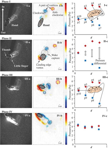
Figure 5. Flow velocities (black arrows) generated during the one kick cycle within a still water fixed window of 1 × 1 m. The time sequence shows the vortex above the shank from the creation to the destruction, the white open arrows at the legs show the motion of the appendage. The curved open arrows visualise rotation. Because of the flexion of the knee (a), a vortex is generated in the dorsal side of the knee region (b) and separated (c). After the lower reversal point, the legs move upwards (d) and kick into the vortex (e) for propulsion (vortex re-capturing) (Hochstein & Blickhan, 2011).

The merits of PIV are summarised as follows: (i) the method does not disturb the swimming motion owing to its contact-free setup; (ii) instantaneous velocity, vorticity and heat-flux rates can be measured; and (iii) multidimensional measurements are possible. The demerits are as follows: (i) it takes a long time to calibrate the flow field; (ii) the time resolution is poor (up to 15 Hz); and (iii) the dynamic range of the velocity is low. The most serious issue with PIV appears to be the inherent limitations in the area of observation, and even in the latest studies, the observation area is limited to two dimensions and 1 m². The latter is clearly not sufficient to cover the entire swimming motion at once. To solve this problem, improvements in the output range of the laser sheet are essential.

Despite these issues, the important role of PIV remains in the improvement and validation of CFD. The momentum of flow can be calculated by PIV and the data used to adjust the CFD models to so that the simulations match experimentally obtained fluid motion and momentum of vortices.

4. Swimming human simulation model (SWUM)

Although PIV is a very powerful tool to understand the flow field around a swimmer in detail, it can be used only to analyse the actual (happened) phenomena. It cannot be used to predict what will happen in unknown (unmeasured) situations, for example to predict how much the resultant swimming speed will change if a joint angle is changed by 5°. For such predictions, computer simulations are very useful since it is possible to change only parameters of focus and to quantify the effect of those parameters. However, computer simulation based on CFD is not suitable for such prediction since the computation time becomes generally enormous. It takes too much computation time to conduct large-scale parameter study or parameter optimisation using CFD. Therefore, an alternative computer simulation method that requires much less computation time than CFD has been developed by Nakashima, Satou, and Miura (2007). This method is called SWUM. The model takes account of the added mass and unsteady fluid forces, including buoyancy and gravity. Figure 6 shows schematically the analytical model of the human body. The latter is represented as a series of truncated elliptic cones. The equation of the motion of the human body for the translational direction in the absolute coordinate system (O-xyz) (Figure 6(a)) is given by

(3)

Figure 6. Illustration of the principles of SWUM: (a) analytical model of swimming human; (b) an example of body geometry (male, 20–29 years); (c) fluid forces except buoyancy; (d) buoyancy is calculated by integrating pressure force on divided quadrangles; (e) divided elliptic plate; and (f) judgement whether quadrangles submerge or not (Nakashima et al., 2007).

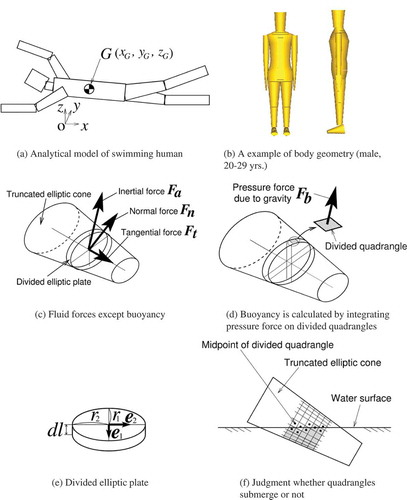
where m_j is the mass of the jth truncated elliptic cone, x_G is the displacement vector of the human’s centre of mass G and F_j is the external force vector acting on the jth cone. The human body is modelled as 21 segments representing the head, neck, shoulders, chest (upper and lower), waist (upper and lower), hips (upper and lower), upper arms, forearms, hands, thighs, shank and feet (Figure 6(b)). As the fluid force components act on each truncated elliptic cone, the inertial force due to added mass of fluid (F_a), drag forces normal (F_n) and tangential (F_t) to the longitudinal direction, and buoyancy are taken into account. Each truncated elliptic cone is divided into thin elliptic plates along the longitudinal axis, as shown in Figure 6(c), and all the fluid force components except buoyancy are assumed to act on each centre of the thin elliptic plates. Buoyancy (F_b), on the other hand, is calculated by integrating the pressure force due to the gravitational force acting on the tiny quadrangle, into which the surface of the thin elliptic plate is again divided in the circumferential direction, as shown in Figure 6(d). Note that the buoyancy is calculated only for the submerged tiny quadrangles. All the fluid forces except buoyancy are assumed to be computable from the local position, direction, velocity and acceleration of the centre of each divided thin elliptic plate. For example, the acceleration is used to calculate the inertial force due to added mass of fluid, while the velocity is used to calculate the normal and tangential drag forces. Each fluid force component has its fluid force coefficient in the formulation. These fluid force coefficients can adjust the magnitudes of the estimated fluid forces, and have been determined from the experimental results.

The fluid force model in SWUM has been found to be within 7.5% error against the experimental values (Nakashima, 2007; Nakashima et al., 2007). The simulated fluid forces acting on the limbs sufficiently reproduced the experimental results for all the experimental conditions, although some discrepancies were observed for the motion close to the water surface or at the start or end of a cycle (Nakashima & Takahashi, 2012a, 2012b). The overall performance of the simulation using the determined fluid force coefficients to predict the time variation of the fluid forces was satisfactory (Nakashima & Ejiri, 2012).

The fluid forces acting on the swimmer can be calculated by SWUM without solving the flow field. Therefore, the computation time generally becomes much smaller than CFD enabling large-scale parameter studies as well as the optimising calculations. However, SWUM is limited in that it considers neither the effects of the surrounding walls nor the mutual interaction of limbs; thus, the computational results of SWUM might differ from those of CFD. A comparative review of SWUM and CFD is required in further studies.

Nakashima and his group have performed simulations of various swimming motions using SWUM, including the front crawl (Nakashima & Ono, 2014; Nakashima, 2007; Nakashima, Maeda, Miwa, & Ichikawa, 2012); breaststroke (Nakashima, Hasegawa, Kamiya, & Takagi, 2013); comparison of the four strokes (Nakashima, 2008); underwater undulation swimming (Nakashima, 2009); monofin swimming (Nakashima, Suzuki, & Nakajima, 2010); and dive starts (Kiuchi, Nakashima, Cheng, & Hubbard, 2010). These simulations have provided practical information for adjusting swimming movements to enable a human to swim faster. Recently, SWUM was utilised not only for the objective of swimming faster but also for a transfemoral prosthesis for the swimming of persons with lower-limb amputations (Nakashima, Suzuki, Ono, & Nakamura, 2013). Further applications, for example the product development of swimwear or tools which contribute to swimming easily, can be expected.

5. Direct measurement of unsteady fluid forces using robotics

Although sophisticated methodologies such as CFD, PIV and SWUM have come into practical use in swimming research, the direct measurement of forces and pressures is still important to verify the results by these methodologies.

Takagi and his colleagues (Takagi & Sanders, 2002; Takagi & Wilson, 1999; Tsunokawa, Nakashima, Sengoku, Tsubakimoto, & Takagi, 2014) have developed a methodology to estimate fluid dynamic forces acting on a hand or foot during swimming by pressure distribution measurement. The pressure measurements (Takagi & Sanders, 2002) appear to have reliability higher than those from the conventional quasi-steady-state method (Berger, de-Groot, & Hollander, 1995; Schleihauf, 1979) and are useful to validate the results computed using CFD.

Nakashima et al. (Nakashima & Takahashi, 2012a, 2012b) developed an underwater robotic arm that has five degrees of freedom to perform the various complicated limb motions that occur during swimming. Using the robotic arm, unsteady fluid force actions on a hand or a foot were directly measured, and the resulting data were analysed with SWUM to improve the computational results. Nakashima and his group also developed a humanoid robot (Chung & Nakashima, 2013a, 2013b), which was designed to be able to perform the motion of the front crawl autonomously in a swimming pool. After various improvements, the humanoid robot could swim by itself at 0.2–0.24 m · s^–1 (Figure 7). Using this approach, we may expect to understand the mechanisms by which unsteady fluid forces develop, and thereby make recommendations to increase speed. Takagi collaborated with Nakashima and Matsuuchi to measure pressures using pressure sensors and flow field measurement by PIV during a simple 2D motion of a robotic arm in water, to understand the interactions among pressures, forces and the flow field (Takagi, Nakashima, Ozaki, & Matsuuchi, 2013). They concluded that when the maximum resultant force acted on the hand, a pair of counter-rotating vortices appeared on the dorsal surface of the hand. The vortex attached to the hand increased the flow velocity, which led to a decrease in surface pressure and an increase in hydrodynamic force. This phenomenon is known as the unsteady mechanism of force generation (Figure 8). Takagi et al. (2013) determined that the drag and lift forces were 72% and 4.8 times greater than the values estimated under steady flow conditions, respectively.

Figure 7. Overview of swimming motion generation (Chung & Nakashima, 2013a, 2013b).

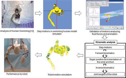
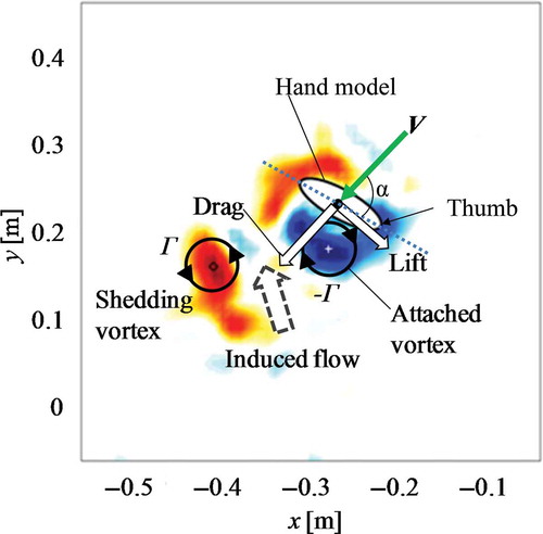
Figure 8. A frame format of interactions among vortices, induced flow and hydrodynamic forces when maximum resultant fluid forces occurred. V expresses the relative velocity vector towards a hand, and the angle of attack (α) was equivalent to approximately 80°. When the hand starts at such a high angle of attack, the rapidly increasing circulation does not remain bound to the hand but rather forms an attached vortex on the leading edge. As swimming proceeds, the leading-edge vortex is eventually shed from the hand. This shedding is known as Von Karman vortex shedding, and its magnitude of circulation is denoted by Γ. The shedding vortex induces a jet flow between the dorsal side of the hand and the vortex, which further re-attaches to the thumb side vortex. By Kelvin’s circulation theorem, the magnitude of circulation about the attached vortex on the dorsal side increases with an increasing negative value of the shedding vortex (−Γ). In consequence, the pressure in the dorsal side declines drastically (Takagi et al., 2013).

6. Integration of knowledge in front crawl analyses

Although each of the aforementioned methodologies has its own merits, integrating knowledge from each of the different methodologies is necessary, because the information provided by one method can “fill the gaps” in information provided by other methods or overcome the weaknesses of another method. Therefore, we attempt to integrate the results obtained from front crawl analyses because this style of swimming is the most complex stroke and the one most commonly used, that is in training as well as in competition. The integrated approach could be applied to any swimming stroke.

Sato and Hino (2003, 2013) performed a 3D CFD simulation for the front crawl stroke of two competitive swimmers using the moving grid approach via the SURF code. In their recent work (Sato & Hino, 2013), the stroke paths measured by stereo cameras were used for the simulation, and the transient forces acting on a hand were predicted (Figure 9) together with the thrust efficiency. In this simulation, all the transient effects (i.e. acceleration, rotation and curved stroke path) were taken into account. The code was validated by comparison with measurements for unsteady flow performed by Kudo, Vennell, Wilson, Waddell, and Sato (2008). According to the CFD result for Ian Thorpe (Figure 9(a)), a successful competitive swimmer, when he was advancing at 1.84 m· s^–1, the mean resultant force, mean thrust force and thrust efficiency generated by his hand were 63.9 N, 32.4 N and 50.7%, respectively (Sato & Hino, 2013). Of particular note was an upsweep phase in the latter part of the stroke so that the generated resultant force of his hand contributed to propulsion with zero waste, as shown in Figure 9(a) and, interestingly, links to the high elbow technique as contributing to his efficiency (Adams, 2000).

Figure 9. Hydrodynamic forces acting on a hand during freestyle stroke computed with CFD. Strokes of Ian Thorpe (a) and Peter Van den Hoogenband (b) at 175 m in a race of 200 m (Sato & Hino 2013).

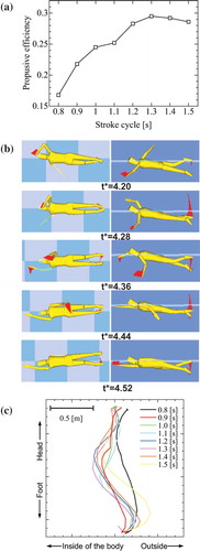
To assess the effectiveness of the high elbow technique, Nakashima et al. (2012) studied computationally the optimal arm strokes during front crawl that maximise the propulsive efficiency and swimming speed. For this objective, an optimisation method that consisted of a random search and the particle swarm optimisation algorithm (Eberhart & Kennedy, 1995) was constructed. To consider the muscle strength characteristics of the swimmer as the constraint condition of the optimisation, maximum joint torques obtained experimentally for various joint angles and angular speeds provided a database to perform the optimisation calculation. The results showed that optimal (maximum) propulsion efficiency occurred when the stroke cycle was 1.3 s. The efficiency reached about 29% as shown in Figure 10(a). The locus of the hand tip drew the so-called S-shaped curve (as viewed from above) and the illustrations of whole body motion demonstrated “high elbow technique” as shown in Figure 10(b). In this case, the swimming speed reached 1.71 m · s^–1. These results are in close agreement with finalists’ average values in the men’s 200 m freestyle in the 10th FINA World Championships of 2013 in Barcelona which were 1.37 s for the stroke cycle and 1.78 m · s^–1 for the swimming speed. The optimal (maximum) swimming speed occurred when the stroke cycle was 0.9 s (red line in Figure 10(c)). In this case, the locus of hand tip appeared “I-shaped” rather than “S-shaped”. The close match between simulation outcomes and swimmers’ actual techniques in practice is encouraging.

Figure 10. Results of optimisation calculation by using SWUM. (a) Relationship between stroke cycle time (T) and propulsive efficiency; (b) bottom view (left) and side view (right) of swimming motions at maximising propulsive efficiency (T = 1.3 s); and (c) loci of left hand tip for various stroke cycles at maximising swimming velocity while the stroke cycle time (T) varied from 0.8 to 1.3 s (Nakashima et al., 2012).

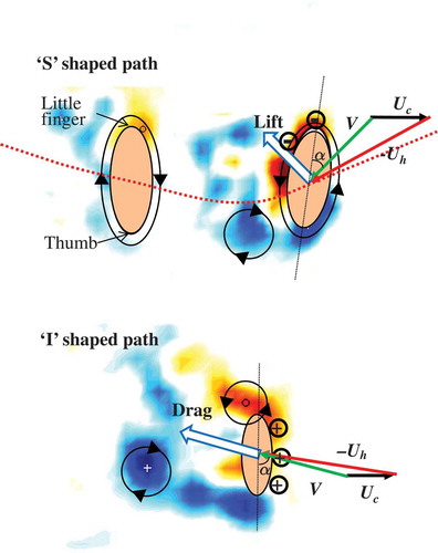
To investigate the differences in propulsion achieved by “S-shaped” and “I-shaped” hand paths, Takagi, Nakashima, Ozaki, and Matsuuchi (2014) performed measurements for a hand attached to a robotic arm with five degrees of freedom, and the hand and arm were independently controlled by a computer. The computer was programmed so that the hand and arm mimicked the front crawl. They directly measured forces on the hand, as well as pressure distributions; underwater flow fields near the hand were obtained via 2D PIV. They identified two important mechanisms (see Figure 11). The first is an unsteady lift force generated when the hand changed direction when scribing the “S”, leading to vortex shedding and the creation of a bound vortex around it. This bound vortex circulation results in a lift force that contributed to thrust in the swimming direction. The second is the generation of a Kármán vortex street when the hand moved linearly with a large angle of attack when scribing the “I” stroke pattern. When the vortices in this street are shed, a drag force was produced that contributed to the thrust. Thus, it may be concluded that professional swimmers can benefit from both an “S”-shaped hand path and an “I”-shaped hand path.

Figure 11. Conceptual diagrams of hydrodynamic forces acting on the hand during ‘S’ shaped (upper panel) and ‘I’ shaped (lower panel). By the end of insweep in ‘S’ shaped, a clockwise vortex has formed near the thumb. As the hand changes from insweep to upsweep, this vortex sheds, forming a counterclockwise-bound vortex around the hand. This circulatory flow combines with the thrust, producing lift on the hand. In ‘I’ shaped, near the middle of the motion at which the thrust is maximum, a Kármán vortex street has formed from which clockwise and counterclockwise vortices are alternatively shed from the hand. At this point, the pressure difference between the dorsal and palm sides of the hand are large, producing drag that contributes to the thrust (Takagi et al., 2014a).

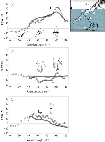
In the “quasi-static” approach to estimate forces produced by a hand (Berger et al., 1995; Schleihauf, 1979), only hand speed and orientation to the flow were considered. However, by measuring forces acting on an accelerating hand Sanders (1999) showed that accelerations have large effects on the total force and so must be considered in addition to the instantaneous speed when estimating forces from time records of hand motion. Recently, this work has been extended by Kudo, Vennell, and Wilson (2013) who investigated the effect of hand acceleration on force generation during the front crawl arm motion. Using a hand–forearm model attached to a triaxial load cell, they determined that the hydrodynamic forces acting on an accelerating hand varied between 1.7 and 25 times the forces on a non-accelerating hand calculated by the quasi-steady-state method (Figure 12). They also found irregular oscillations in the forces produced by an accelerating hand and proposed that these were due to vortex shedding from the side of the little finger or the thumb. This suggestion has been confirmed by the experiments of Takagi, Nakashima et al. (2014) using robotic arms. They observed the generation of a Kármán vortex street under similar conditions.

Figure 12. (a) Drag force acting on the hand (D); (b) transverse lift force acting on the hand in the x direction (L_T); and (c) lift force in the dorsal direction acting on the hand perpendicular to the drag and transverse lift forces (L_D) in the flowing flume set at 1.5 m · s^–1. In (a), (b) and (c), the empty circles (○) represent hydrodynamic forces on the hand measured during acceleration, and the filled circles (●) represent hydrodynamic forces calculated for a non-accelerating hand. The hands in the figures show orientations, while the arrow with the hand represents the direction of the hydrodynamic force acting on the hand at the respective φ (Kudo et al., 2013).

By reviewing these studies, we have found two important issues relating to swimming research: a mechanism of generating unsteady fluid forces and a theory to enable faster and more efficient swimming. For the generation of unsteady fluid forces, vortex generation plays an important role. According to the results of Kudo et al. (2013), irregular oscillations occur in the hydrodynamic forces while the hand is accelerating. Takagi, Nakashima et al. (2014) suggested that these oscillations were caused by a Kármán vortex street, that is a phenomenon when clockwise or counterclockwise vortices were alternately shed from the side of the little finger or the thumb. Such Kármán vortex street is known to be generated when the hand moves in a linear manner with a large angle of attack as in the “I-shaped” stroking pattern. At that time, the pressure on the palm side becomes positive, while that on the dorsal side becomes negative, and the pressure difference between the palm and dorsal sides increases, producing a drag force (upper panel in Figure 11). This drag force contributes to an increase in the thrust force. Another mechanism has been suggested to contribute to the generation of unsteady lift forces, for example by changing the leading edge of the hand (Takagi, Nakashima et al., 2014). When the leading edge changes from the side of the thumb to the little finger, the direction of the bound vortex of the hand changes from clockwise to counterclockwise because of a shedding vortex from the side of the thumb. By adding this circulation to the moving velocity, the surface velocity increases, the surface pressure decreases and a lift force is produced (lower panel in Figure 11). This phenomenon has been confirmed by experiments which measured the velocity field during front crawl with 3D motion analysis (Matsuuchi & Muramatsu, 2011); thus, excellent swimmers also gain propulsion from this unsteady lift force.

In terms of a theory for swimming faster or more efficiently, the results of Nakashima et al. (2012) give us some important suggestions. Increasing stroke frequency (f_s) is essential to increase swimming speed (U_s), which is consistent with the results of Craig and Pendergast (1979) who found that U_s is proportional to f_s. However, a swimmer cannot, of course, increase f_s limitlessly because of a limitation of muscle power or stroke coordination. Nakashima et al. (2012) also found that U_s decreased conversely when f_s exceeded the optimum frequency because of the muscle strength characteristics, that is the swimmer in the simulation could not produce a large joint torque during a motion that could exceed a certain threshold. For the fastest case, the stroke pattern appears to be the so-called I-shaped stroke. Therefore, in the 50 m or 100 m freestyle event in which speed is more important than efficiency, it might be better for a swimmer to increase f_s by using a “straight pull” (Figure 10(c)). Alternatively, to improve propulsion efficiency, a swimmer should use a “high elbow” and scribe an “S-shaped” pattern (Figure 10(b)) similar to that of Ian Thorpe’s.

7. Conclusion

By reviewing the available literature, both numerical and experimental, relating to swimming, we have seen that studies based on the CFD approach have the potential to provide new insights and to provide information that cannot be obtained by testing and measurement. Similarly, SWUM simulations offer practical benefits to coaches and swimmers by providing information regarding the optimal movements for improved training and performance. In addition, PIV measurements play a vital role in verifying results from numerical simulations. Furthermore, applying a combination of these methods will be a powerful tool to further advance research in swimming.

Acknowledgements

The authors thank all members of Swimming Laboratory at the University of Tsukuba for their contributions to the experiments and data analysis discussed in this article. We also extend our thanks to Dr. Shigetada Kudo and Dr. Georgios Machtsiras for their help in offering us the relevant data.

Disclosure statement

No potential conflict of interest was reported by the authors.

References

- Adams, M. (2000). Thoughts on the crawl stroke. Swimming Technique, 37(2), 17–23.
- Adrian, R. J. (1991). Particle-imaging techniques for experimental fluid mechanics. Annual Review of Fluid Mechanics, 23(1), 261–304.
- Alves, F., Marinho, D., Leal, L., Rouboa, A., & Silva, A. (2007). 3D computational fluid dynamics of the hand and forearm in swimming. Medicine & Science in Sports & Exercise, 39(5), S9.
- Berger, M. A. M., de-Groot, G., & Hollander, A. P. (1995). Hydrodynamic drag and lift forces on human hand/arm models. Journal of Biomechanics, 28(2), 125–133.
- Bilinauskaite, M., Mantha, V. R., Rouboa, A. I., Ziliukas, P., & Silva, A. J. (2013). Computational fluid dynamics study of swimmer’s hand velocity, orientation, and shape: Contributions to hydrodynamics. Biomed Research International. Advance online publication. doi:10.1155/2013/140487
- Bixler, B., Pease, D., & Fairhurst, F. (2007). The accuracy of computational fluid dynamics analysis of the passive drag of a male swimmer. Sports Biomechanics, 6(1), 81–98.
- Bixler, B., & Riewald, S. (2002). Analysis of a swimmer’s hand and arm in steady flow conditions using computational fluid dynamics. Journal of Biomechanics, 35, 713–717.
- Bixler, B., & Schloder, M. (1996). Computational fluid dynamics: An analytical tool for the 21st century swimming scientist. Journal of Swimming Research, 11, 4–22.
- Chung, C., & Nakashima, M. (2013a). Development of a swimming humanoid robot for research of human swimming. Journal of Aero Aqua Bio-mechanisms, 3(1), 109–117.
- Chung, C., & Nakashima, M. (2013b). Free swimming of the swimming humanoid robot for the crawl stroke. Journal of Aero Aqua Bio-mechanisms, 3(1), 118–126.
- Cohen, R. C., Cleary, P. W., & Mason, B. (2012). Simulations of dolphin kick swimming using smoothed particle hydrodynamics. Human Movement Science, 31(3), 604–619.
- Craig, A. B., & Pendergast, D. R. (1979). Relationships of stroke rate, distance per stroke, and velocity in competitive swimming. Medicine and Science in Sports and Exercise, 11(3), 278–283.
- Dickinson, M. H., Lehmann, F.-O., & Sane, S. P. (1999). Wing rotation and the aerodynamic basis of insect flight. Science, 284(5422), 1954–1960.
- Drucker, E. G., & Lauder, G. V. (1999). Locomotor forces on a swimming fish: Three-dimensional vortex wake dynamics quantified using digital particle image velocimetry. Journal of Experimental Biology, 202(18), 2393–2412.
- Eberhart, R. C., & Kennedy, J. (1995). A new optimizer using particle swarm theory. Paper presented at the Proceedings of the sixth international symposium on micro machine and human science.
- Fearing, R. S., Chiang, K. H., Dickinson, M. H., Pick, D., Sitti, M., & Yan, J. (2000). Wing transmission for a micromechanical flying insect. Paper presented at the IEEE International Conference on Robotics and Automation 2000, San Francisco.
- Ferziger, J. H., & Perić, M. (2012). Computational methods for fluid dynamics. Berlin: Springer.
- Gardano, P., & Dabnichki, P. (2006). On hydrodynamics of drag and lift of the human arm. Journal of Biomechanics, 39, 2767–2773.
- Gibson, M. M., & Launder, B. E. (1978). Ground effects on pressure fluctuations in the atmospheric boundary layer. Journal of Fluid Mechanics, 86(03), 491–511.
- Harlow, F. H. (2004). Fluid dynamics in group T-3 Los Alamos national laboratory: (LA-UR-03-3852). Journal of Computational Physics, 195(2), 414–433.
- Hirt, C., Amsden, A. A., & Cook, J. (1974). An arbitrary Lagrangian-Eulerian computing method for all flow speeds. Journal of Computational Physics, 14(3), 227–253.
- Hochstein, S., & Blickhan, R. (2011). Vortex re-capturing and kinematics in human underwater undulatory swimming. Human Movement Science, 30(5), 998–1007.
- Hochstein, S., Pacholak, S., Brücker, C., & Blickhan, R. (2012). Experimental and numerical investigation of the unsteady flow around a human underwater undulating swimmer. In C. Tropea & H. Bleckmann (Eds.), Nature-inspired fluid mechanics (pp. 293–308). Berlin: Springer.
- Kamata, E., Miwa, T., Matsuuchi, K., Shintani, H., & Nomura, T. (2006). Analysis of sculling propulsion mechanism using two-components particle image velocimetry. In J. P. Vilas-Boas, F. Alves, & A. Marques (Eds.), Biomechanics and medicine in swimming X (pp. 50–52). Porto: University of Porto.
- Kawai, M. (1997). Precision engineering for sports (special issue on competitive sports and precision engineering). Journal of the Japan Society of Precision Engineering, 63(4), 455–459.
- Keys, M. (2010). Establishing Computational Fluid Dynamics models for swimming technique (Doctor of Philosophy). Doctoral Dissertation in The University of Western Australia, Perth, Australia.
- Kiuchi, H., Nakashima, M., Cheng, K. B., & Hubbard, M. (2010). Modeling fluid forces in the dive start of competitive swimming. Journal of Biomechanical Science and Engineering, 5(4), 314–328.
- Kleinstreuer, C. (1997). Engineering fluid dynamics—an interdisciplinary systems approach. Cambridge: Cambridge University Press.
- Kudo, S., Vennell, R., & Wilson, B. (2013). The effect of unsteady flow due to acceleration on hydrodynamic forces acting on the hand in swimming. Journal of Biomechanics, 46(10), 1697–1704.
- Kudo, S., Vennell, R., Wilson, B., Waddell, N., & Sato, Y. (2008). Influence of surface penetration on measured fluid force on a hand model. Journal of Biomechanics, 41, 3502–3505.
- Kudo, S., Yanai, T., Wilson, B., Takagi, H., & Vennell, R. (2008). Prediction of fluid forces acting on a hand model in unsteady flow conditions. Journal of Biomechanics, 41, 1131–1136.
- Larsson, L., Stern, F., & Visonneau, M. (2014). Numerical ship hydrodynamics: An assessment of the Gothenburg 2010 workshop. Netherlands: Springer.
- Launder, B. E., & Spalding, D. B. (1972). Lectures in mathematical models of turbulence. London: Academic Press.
- Lecrivain, G., Slaouti, A., Payton, C., & Kennedy, I. (2008). Using reverse engineering and computational fluid dynamics to investigate a lower arm amputee swimmer’s performance. Journal of Biomechanics, 41(13), 2855–2859.
- Lyttle, A., & Keys, M. (2004). The use of computational fluids dynamics to optimise underwater kicking performance. Paper presented at the 22 International Symposium on Biomechanics in Sports, Ottawa.
- Machtsiras, G. (2012). Utilizing Flow Characteristics to Increase Performance in Swimming (Doctor of Philosophy). Doctoral Dissertation in The University of Edinburgh, Edinburgh.
- Marinho, D., Barbosa, T., Rouboa, A., & Silva, A. (2011). The hydrodynamic study of the swimming gliding: A two-dimensional computational fluid dynamics (CFD) analysis. Journal of Human Kinetics, 29(1), 49–57.
- Marinho, D. A., Barbosa, T. M., Reis, V. M., Kjendlie, P. L., Alves, F. B., Vilas-Boas, J. P., … Rouboa, A. I. (2010). Swimming propulsion forces are enhanced by a small finger spread. Journal of Applied Biomechanics, 26(1), 87–92.
- Marinho, D. A., Reis, V. M., Alves, F. B., Vilas-Boas, J. P., Machado, L., Silva, A. J., & Rouboa, A. I. (2009a). Hydrodynamic drag during gliding in swimming. Journal of Applied Biomechanics, 25(3), 253–257.
- Marinho, D. A., Rouboa, A. I., Alves, F. B., Vilas-Boas, J. P., Machado, L., Reis, V. M., & Silva, A. J. (2009b). Hydrodynamic analysis of different thumb positions in swimming. Journal of Sports Science & Medicine, 8(1), 58.
- Matsuuchi, K., Miwa, T., Nomura, T., Sakakibara, J., Shintani, H., & Ungerechts, B. E. (2004). Unsteady flow measurement around a human hand in swimming using PIV. Paper presented at the 9th annual congress of the European College of Sport Science, Clermont-Ferrand, France.
- Matsuuchi, K., Miwa, T., Nomura, T., Sakakibara, J., Shintani, H., & Ungerechts, B. E. (2009). Unsteady flow field around a human hand and propulsive force in swimming. Journal of Biomechanics, 42(1), 42–47.
- Matsuuchi, K., & Muramatsu, Y. (2011). Investigation of the unsteady mechanism in the generation of propulsive force while swimming using a synchronized flow visualization and motion analysis system. In V. Klika (Ed.), Biomechanics in applications (pp. 389–408). Rijeka, Croatia: InTech.
- Minetti, A. E., Machtsiras, G., & Masters, J. C. (2009). The optimum finger spacing in human swimming. Journal of Biomechanics, 42(13), 2188–2190.
- Mittal, R., & Iaccarino, G. (2005). Immersed boundary methods. Annual Review of Fluid Mechanics, 37(1), 239–261.
- Miwa, T., Matsuuchi, K., Sakakibara, J., Shintani, H., Kamata, E., & Nomura, T. (2005). Visualization of dolphin-kicking wake using 3C-PIV method. Paper presented at the 10th annual Congress of the European College of Sport Science, Belgrade.
- Miwa, T., Matsuuchi, K., Shintani, H., Kamata, E., & Nomura, T. (2006). Unsteady flow measurement of dolphin kicking wake in sagittal plane in 2C-PIV. In J. P. Vilas-Boas, F. Alves, & A. Marques (Eds.), Biomechanics and medicine in swimming X (pp. 64–66). Porto: University of Porto.
- Monaghan, J. J. (2012). Smoothed particle hydrodynamics and its diverse applications. Annual Review of Fluid Mechanics, 44(1), 323–346.
- Muramatsu, Y., Matsuuchi, K., Nomura, T., Sakakibara, J., & Miwa, T. (2008). Development of a synchronized system of PIV and motion analysis, and its application to a front crawl swimmer. Paper presented at the 13th annual Congress of the European College of Sport Science, Estoril, Portugal.
- Nagayama, K., Tanaka, T., Tanaka, K., Hayami, H., & Aramaki, S. (2008). Visualization of flow and vortex structure around a swimming loach by dynamic stereoscopic PIV. Experiments in Fluids, 44(5), 843–850.
- Nakashima, M. (2006). “SWUM” and “SWUMSUIT” -A modeling technique of a self-propelled swimmer-. In J. P. Vilas-Boas, F. Alves, & A. Marques (Eds.), Biomechanics and medicine in swimming X (pp. 66–68). Porto: University of Porto.
- Nakashima, M. (2007). Mechanical study of standard six beat front crawl swimming by using swimming human simulation model. Journal of Fluid Science and Technology, 2(1), 290–301.
- Nakashima, M. (2008). Analysis of breast, back and butterfly strokes by the swimming human simulation model SWUM bio-mechanisms of swimming and flying (pp. 361–372). New York, NY: Springer.
- Nakashima, M. (2009). Simulation analysis of the effect of trunk undulation on swimming performance in underwater dolphin kick of human. Journal of Biomechanical Science and Engineering, 4(1), 94–104.
- Nakashima, M., & Ejiri, Y. (2012). Measurement and modeling of unsteady fluid force acting on the trunk of a swimmer using a swimmer mannequin robot. Journal of Fluid Science and Technology, 7(1), 11–24.
- Nakashima, M., Hasegawa, T., Kamiya, S., & Takagi, H. (2013). Musculoskeletal simulation of the breaststroke. Journal of Biomechanical Science and Engineering, 8(2), 152–163.
- Nakashima, M., Maeda, S., Miwa, T., & Ichikawa, H. (2012). Optimizing simulation of the arm stroke in crawl swimming considering muscle strength characteristics of athlete swimmers. Journal of Biomechanical Science and Engineering, 7(2), 102–117.
- Nakashima, M., & Ono, A. (2014). Maximum joint torque dependency of the crawl swimming with optimized arm stroke. Journal of Biomechanical Science and Engineering, 9(1), 1–9.
- Nakashima, M., Satou, K., & Miura, Y. (2007). Development of swimming human simulation model considering rigid body dynamics and unsteady fluid force for whole body. Journal of Fluid Science and Technology, 2(1), 56–67.
- Nakashima, M., Suzuki, S., & Nakajima, K. (2010). Development of a simulation model for monofin swimming. Journal of Biomechanical Science and Engineering, 5(4), 408–420.
- Nakashima, M., Suzuki, S., Ono, A., & Nakamura, T. (2013). Development of the transfemoral prosthesis for swimming focused on ankle joint motion. Journal of Biomechanical Science and Engineering, 8(1), 79–93.
- Nakashima, M., & Takahashi, A. (2007, 2007/7/1–2007/7/5). Measurement of unsteady fluid force acting on limbs in swimming using a robot arm. Paper presented at the International Society of Biomechanics XXI, Taipei International Convention Center, Taiwan.
- Nakashima, M., & Takahashi, A. (2012a). Clarification of unsteady fluid forces acting on limbs in swimming using an underwater robot arm (2nd report, modeling of fluid force using experimental results). Journal of Fluid Science and Technology, 7(1), 114–128.
- Nakashima, M., & Takahashi, A. (2012b). Clarification of unsteady fluid forces acting on limbs in swimming using an underwater robot arm (development of an underwater robot arm and measurement of fluid forces). Journal of Fluid Science and Technology, 7(1), 100–113.
- Noack, R. (2005). SUGGAR: A general capability for moving body overset grid assembly. AIAA Paper, 5117, 2005.
- Orszag, S. A., Yakhot, V., Flannery, W. S., Boysan, F., Choudhury, D., Maruzewski, J., & Patel, B. (1993). Renormalization group modeling and turbulence simulations. Paper presented at the International Conference on Near-Wall Turbulent Flows, Arizona.
- Pacholak, S., Hochstein, S., Rudert, A., & Brücker, C. (2014). Unsteady flow phenomena in human undulatory swimming: A numerical approach. Sports Biomechanics, 13, 176–194.
- Popa, C., Zaidi, H., Arfaoui, A., Polidori, G., Taiar, R., & Fohanno, S. (2011). Analysis of wall shear stress around a competitive swimmer using 3D Navier-Stokes equations in CFD. Acta of Bioengineering and Biomechanics, 13(1), 3–11.
- Roach, P. J. (1998). Verification and validation in computational science and engineering. New Mexico: Hermosa Publishers.
- Roache, P. J. (1998). Verification and validation in computational science and engineering. Socorro: Hermosa.
- Rogallo, R. S., & Moin, P. (1984). Numerical simulation of turbulent flows. Annual Review of Fluid Mechanics, 16(1), 99–137.
- Rouboa, A., Silva, A., Leal, L., Rocha, J., & Alves, F. (2006). The effect of swimmer’s hand/forearm acceleration on propulsive forces generation using computational fluid dynamics. Journal of Biomechanics, 39(7), 1239–1248.
- Sakakibara, J., Nakagawa, M., & Yoshida, M. (2004). Stereo-PIV study of flow around a maneuvering fish. Experiments in Fluids, 36(2), 282–293.
- Sanders, R. H. (1999). Hydrodynamic characteristics of a swimmer’s hand. Journal of Applied Biomechanics, 15(1), 3–26.
- Sato, Y., & Hino, T. (2003). Estimation of thrust of swimmer’s hand using CFD. Paper presented at the Proceedings of the Second International Symposium on Aero Aqua Bio-Mechanisms, Hawaii.
- Sato, Y., & Hino, T. (2010). CFD simulation of flows around a swimmer in a prone glide position. Japanese Journal of Sciences in Swimming and Water Exercise, 13(1), 1–9.
- Sato, Y., & Hino, T. (2013). A computational fluid dynamics analysis of hydrodynamic force acting on a swimmer’s hand in a swimming competition. Journal of Sports Science and Medicine, 12(4), 679–689.
- Schleihauf, R. E. (1979). A hydrodynamic analysis of swimming propulsion. In J. Terauds & E. W. Bedingfield (Eds.), Swimming III (pp. 173–184). Baltimore, MD: University Park Press.
- Silva, A. J., Rouboa, A., Moreira, A., Reis, V. M., Alves, F., Vilas-Boas, J. P., & Marinho, D. A. (2008). Analysis of drafting effects in swimming using computational fluid dynamics. Journal of Sports Science and Medicine, 7(1), 60–66.
- Smagorinsky, J. (1963). General circulation experiments with the primitive equations. Monthly Weather Review, 91(3), 99–164.
- Spalart, P. R., & Allmaras, S. R. (1994). A one-equation turbulence model for aerodynamic flows. Recherche Aerospatiale, 1, 5–21.
- Stern, F., Yang, J., Wang, Z., Sadat-Hosseini, H., & Mousaviraad, M. (2013). Computational ship hydrodynamics: Nowadays and way forward. International Shipbuilding Progress, 60(1–4), 3–105.
- Suhs, N. E., Rogers, S. E., & Dietz, W. E. (2002, June 24–26). Pegasus 5: An automated pre-processor for overset-grid cfd. Paper presented at the 32nd AIAA Fluid Dynamics Conference, AIAA 2002–3186, St. Louis, MO.
- Takagi, H., Nakashima, M., Ozaki, T., & Matsuuchi, K. (2013). Unsteady hydrodynamic forces acting on a robotic hand and its flow field. Journal of Biomechanics, 46(11), 1825–1832.
- Takagi, H., Nakashima, M., Ozaki, T., & Matsuuchi, K. (2014). Unsteady hydrodynamic forces acting on a robotic arm and its flow field: Application to the crawl stroke. Journal of Biomechanics, 47(6), 1401–1408.
- Takagi, H., & Sanders, R. (2002). Propulsion by the hand during competitive swimming. In S. Ujihashi & S. J. Haake (Eds.), The engineering of sport 4 (pp. 631–637). Oxford: Blackwell Publishing.
- Takagi, H., Shimada, S., Miwa, T., Kudo, S., Sanders, R., & Matsuuchi, K. (2014). Unsteady hydrodynamic forces acting on a hand and its flow field during sculling motion. Human Movement Science, 38, 133–142.
- Takagi, H., & Wilson, B. (1999). Calculating hydrodynamic force by using pressure differences in swimming. In K. L. Keskinen, P. V. Komi, & A. P. Hollander (Eds.), Biomechanics and medicine in swimming VIII (pp. 101–106). Jyväskylä: Gummerus Printing.
- Tsunokawa, T., Nakashima, M., Sengoku, Y., Tsubakimoto, S., & Takagi, H. (2014). A new method to evaluate breaststroke kicking technique using a pressure distribution analysis. In B. Mason (Ed.), Biomechanics and medicine in swimming XI (pp. 263–269). Canberra: Australian Institute of Sports.
- Vennell, R., Pease, D., & Wilson, B. (2006). Wave drag on human swimmers. Journal of Biomechanics, 39(4), 664–671.
- von Loebbecke, A., & Mittal, R. (2012). Comparative analysis of thrust production for distinct arm-pull styles in competitive swimming. Journal of Biomechanical Engineering, 134(7), 074501–074504.
- von Loebbecke, A., Mittal, R., Fish, F., & Mark, R. (2009a). A comparison of the kinematics of the dolphin kick in humans and cetaceans. Human Movement Science, 28(1), 99–112.
- von Loebbecke, A., Mittal, R., Fish, F., & Mark, R. (2009b). Propulsive efficiency of the underwater dolphin kick in humans. Journal of Biomechanical Engineering, 131(5), 54504.
- Von Loebbecke, A., Mittal, R., Mark, R., & Hahn, J. (2009c). A computational method for analysis of underwater dolphin kick hydrodynamics in human swimming. Sports Biomechanics, 8(1), 60–77.
- Wei, T., Mark, R., & Hutchison, S. (2014). The fluid dynamics of competitive swimming. Annual Review of Fluid Mechanics, 46, 547–565.
- Wilcox, D. C. (1988). Reassessment of the scale-determining equation for advanced turbulence models. AIAA Journal, 26(11), 1299–1310.
- Yamada, K., Matsuuchi, K., Nomura, T., Sakakibara, J., Shintani, H., & Miwa, T. (2006). Motion analysis of front crawl swimmer’s hand and the visualization of flow fields using PIV. In J. P. Vilas-Boas, F. Alves, & A. Marques (Eds.), Biomechanics and medicine in swimming X (pp. 111–113). Porto: University of Porto.
- Zaidi, H., Fohanno, S., Taiar, R., & Polidori, G. (2010). Turbulence model choice for the calculation of drag forces when using the CFD method. Journal of Biomechanics, 43(3), 405–411.
- Zaidi, H., Taiar, R., Fohanno, S., & Polodori, G. (2008). Analysis of the effect of swimmer’s head position on swimming performance using computational fluid dynamics. Journal of Biomechanics, 41, 1350–1358.