Latent variable dose–response modelling of external training load measures and musculoskeletal responses in elite rugby league players

ABSTRACT

Establishing dose–response relationships between training load and fatigue can help the planning of training. The aim was to establish the relative importance of external training load measurements to relate to the musculoskeletal response on a group and individual player level. Sixteen elite male rugby league players were monitored across three seasons. Two- to seven-day exponential weighted averages (EWMA) were calculated for total distance, and individualised speed thresholds (via 30–15 Intermittent Fitness Test) derived from global positioning systems. The sit and reach, dorsiflexion lunge, and adductor squeeze tests represented the musculoskeletal response. Partial least squares and repeated measures correlation analyses established the relative importance of training load measures and then investigated their relationship to the collective musculoskeletal response for individual players through the construction of latent variables. On a group level, 2- and 3-day EWMA total distance had the highest relative importance to the collective musculoskeletal response (p < 0.0001). However, the magnitude of relationships on a group (r value = 0.20) and individual (r value = 0.06) level were trivial to small. The lack of variability in the musculoskeletal response over time suggest practitioners adopting such measures to understand acute musculoskeletal fatigue responses should do so with caution.

KEYWORDS:

• Partial least squares correlation
• fatigue
• training load
• team sports

Introduction

In professional rugby league, the structure of competition and concurrent training programmes mean players complete a variety of different activities (e.g. accelerating, high-speed running, collisions, strength and power programming) – termed the external training load (Impellizzeri et al., 2005). Across a period of training, coaches manipulate the frequency, intensity and duration of the external training load to impose an internal training load that elicits a suitable fitness/fatigue response to maximise favourable training outcomes (e.g. adaptation/performance) (Banister et al., 1975; Impellizzeri et al., 2005). However, in practice, this is extremely difficult to achieve as the internal training load is an abstract latent construct that involves multiple dimensions, given it is defined as the response to the external load across psychological (Soligard et al., 2016), physiological (e.g. oxygen consumption, blood lactate) (Impellizzeri et al., 2005; Soligard et al., 2016) and biomechanical (e.g. cartilage, bone, muscle, tendon; Vanrenterghem et al., 2017) systems. Therefore, for any athlete, the magnitude of the resultant fatigue response for each of these systems is likely mediated by an array of personal characteristics (e.g. training and injury history and psycho-emotional state) and the specific external training load that is prescribed over a period of time (Kiely, 2018; Impellizzeri et al., 2019).

By quantifying the dose–response relationship between the training load prescribed to athletes and their fatigue response, it is hoped that short-term training prescription can be better managed (Impellizzeri et al., 2005; Oxendale et al., 2016; Thorpe et al., 2017). Measurements such as the session-rating-of-perceived-exertion (sRPE), heart rate or microtechnology are often used to represent the training load prescribed (Akenhead & Nassis, 2016). Monitoring the fatigue response often includes cardiovascular measures such as changes in heart rate variability or heart rate response to a controlled bout of running (Scott et al., 2018; Veugelers et al., 2016; Williams et al., 2018) and neuromuscular function measures such as the countermovement jump (Twist & Highton, 2013). Repeated musculoskeletal screening measurements are also popular in applied practice to detect changes in musculoskeletal (rather than physiological/neuromuscular) specific responses such as hip adductors’ strength (Roe et al., 2016) or lower back/hamstring/calf flexibility (e.g. sit and reach [S&R] or dorsiflexion lunge tests [DLT]) (Esmaeili et al., 2018). Overall, coaches and sports scientists collect a variety of measurements to capture the different dimensions of the training load and fatigue constructs but limited attention has been paid to the dose–response relationship between training load and musculoskeletal fatigue responses.

Given the theoretical frameworks of training dose-response, it is likely that a training load variable could be important to understand the fatigue response of one system (e.g. cardiovascular fatigue) but might be unimportant for another (e.g. musculoskeletal fatigue) (Esmaeili et al., 2018; Lonie et al., 2020; Williams et al., 2018). For example, whilst Williams et al. (2018) reported sRPE to explain 44% of the variance in changes in heart rate variability (r = 0.66 ± 0.32) across an 8 week training period in elite rugby 7’s players, both Esmaeili et al. (2018) and Lonie et al. (2020) reported trivial effects of sRPE on the variability of musculoskeletal response scores in elite Australian rules football players. Therefore, there also becomes an increasing requirement to evaluate and then omit training load variables that are deemed unimportant to explain the fatigue response for any given system (i.e. cardiovascular vs. musculoskeletal response) (Vanrenterghem et al., 2017; Weaving et al., 2020). In these examples, given the conceptual differences in the internal training loads required for adaptation between cardiovascular (e.g. ventricular hypertrophy; MacInnis & Gibala, 2017) and musculoskeletal (e.g. tendon stiffness) systems (Vanrenterghem et al., 2017), it is possible that sRPE underrepresents the true internal load imposed on the musculoskeletal system and that external load measurements could provide a better relationship with musculoskeletal response measurements (Esmaeili et al., 2018; Vanrenterghem et al., 2017). For example, Roe et al. (2016) reported that the accumulation of sprint distance (>80% of 40-m maximal sprint speed) during rugby union match play related to immediate (r = −0.52), +24 h (r = −0.47) and +48 h (r = −0.71) changes in adductor squeeze strength in academy rugby union players. This suggests that the external load could provide useful surrogate dose–response relationships with musculoskeletal responses when measured over longitudinal periods, although these relationships have yet to be investigated in any professional team sport.

Another broader consideration is that due to the multidimensional aspects of both the training load and fatigue measurements (e.g. cardiovascular, neuromuscular, musculoskeletal) it can be hard to provide a parsimonious model of their dose–response relationship (Ryan et al., 2020). This is because the variables used to represent different dimensions of the training load and fatigue constructs frequently exhibit considerable multicollinearity (McLaren et al., 2017; Weaving et al., 2019). Consequently, a common approach is to conduct multiple univariate models involving each of the individual measurements (e.g. correlation between total distance and adductor squeeze strength, total distance and ankle dorsiflexion). However, univariate analysis is limited as it assumes that each of the variables are independent and also does not “capture” any information that may be included within the covariance of the datasets. As a result, those models are evaluating the relationships between individual dimensions of the construct, rather than the multidimensional construct as a whole. This can be problematic with training load and fatigue measurements, as the magnitude of covariance differs depending on the training modes prescribed over a training period (McLaren et al., 2017; Weaving et al., 2020). However, orthogonal data analysis approaches, such as singular value decomposition (SVD) (Till et al., 2016) or partial least squares correlation analysis can overcome this issue (PLSCA) (Abdi & Williams, 2013; Weaving et al., 2019). PLSCA has potential to dose–response analyses, as key relationships between datasets that both include multiple variables can be evaluated together within a single analysis. This can enable complex load and response constructs to be evaluated more effectively and visualised more simply (Krishnan et al., 2011; Weaving et al., 2019). Whilst these techniques are regularly utilised in other fields such as chemometrics and genomics (Barker & Rayens, 2003; Liquet et al., 2012), their application has been limited in sports science. Therefore, the primary aim of the current study was to evaluate the relative importance of external load variables to relate to measures of musculoskeletal fatigue response in elite rugby league players through PLSCA. A secondary aim was to assess the extent to which group level (i.e. between-subject) variable importance was applicable to each individual players own dose–response relationship.

Method

Subjects

Sixteen elite male rugby league players (mean ± SD: age 24 ± 4 y body mass, 100.2 ± 8.4 kg, height 182 ± 13 cm) from the same Australian-based National Rugby League (NRL) team were recruited to participate. For players to be included they had to satisfy the strict data exclusion criteria (detailed below). All players provided written voluntary consent to participate in this investigation and the study received institutional ethics approval (approval number: HMNS18/1801).

Design

The study used a longitudinal observational research design in which daily training load and musculoskeletal screening data were collected across three complete NRL seasons (observations; n = 1699). Daily musculoskeletal screening tests were conducted throughout the pre-season (November – February) and competitive (March – October) phases. Exponentially weighted moving averages (EWMA) of the training load variables were calculated across 2- to 7-day periods and that value aligned with the following days musculoskeletal screening tests (Williams et al., 2017). For example, if screening was conducted on Monday in pre-season, the EWMA calculated for each variable on the Sunday would be aligned with this value. This was to ensure that any training load accrued on the same day, but after the completion of the musculoskeletal screening tests, were not included in the calculation of the EWMA.

Methodology

External training load measures

Global positioning system (GPS) data were collected for each training session using 5 Hz interpolated to 15 Hz devices (SPI HPU GPSports, Canberra, Australia). The mean (± SD) number of satellites (12.6 ± 2.7) and horizontal dilution of precision (1.1 ± 0.1) during the data collection period suggest suitable accuracy of the collected data (Malone et al., 2017) . These devices possess acceptable levels of validity (standard error of the mean = 0.07 to 0.14 m·s-1) and reliability (intra-unit: coefficient of variation [CV] = 0.9–2.6%, inter-unit CV = 1.0–7.8%) for high-speed measurements against a timing gate criterion (Barr et al., 2019) alongside acceptable validity for total distance (intraclass correlation coefficient = 0.99) during court-based movements (Tessaro & Williams, 2018). Data from GPS were downloaded following the completion of each training session or match using Team AMS (GPSports, Canberra, Australia) and trimmed to include only active drill or match-play time.

Players completed the 30–15 Intermittent Fitness Test (30–15_IFT) at the beginning and completion of the pre-season period of each season, with the end-stage velocity (V_IFT) used to determine relative speed thresholds. All testing sessions were performed on the same outdoor grass field and at the same time of day (~0700–0900), with players wearing their issued training attire and own football boots. Sessions were performed under similar environmental conditions (21–26°C). Estimates of the first (VT_1IFT; 68% V_IFT = 12.8 ± 0.6 km∙h⁻¹) and second ventilatory (VT_2IFT; 87% V_IFT = 16.6 ± 0.8 km∙h⁻¹) thresholds (Scott et al., 2018) were calculated for each player. The distance (m) covered above each of these thresholds, comparable in the literature to high speed- and very high speed-running, respectively (McLaren et al., 2017), were quantified for each session for each player across the study period. Following each 30–15_IFT testing period, any changes to a players terminal velocity, and therefore their relative running thresholds, were updated within the proprietary software (Team AMS, GPSports, Canberra, Australia). No testing was performed during the competitive phase as 30–15_IFT performance has previously been reported to not change substantially in elite rugby league players across the in-season phase (typical error = 0.42 km·h⁻¹, CV = 1.9%) (Scott et al., 2018).

Exponentially weighted moving average of external training load

On any given day, the EWMA was calculated for total distance, VT_1IFT and VT_2IFT distance for each player as described by Williams et al. (2017). The EWMA for a given day was calculated as per equation 1(1) $\mathrm{E}\mathrm{W}\mathrm{M}{\mathrm{A}}_{\mathrm{t}\mathrm{o}\mathrm{d}\mathrm{a}\mathrm{y}}=\mathrm{L}\mathrm{o}\mathrm{a}{\mathrm{d}}_{\mathrm{t}\mathrm{o}\mathrm{d}\mathrm{a}\mathrm{y}}\mathrm{x}{\lambda }_{\mathrm{a}}+\left(\left(1-{\lambda }_{\mathrm{a}}\right)\mathrm{x}\mathrm{E}\mathrm{W}\mathrm{M}{\mathrm{A}}_{\mathrm{y}\mathrm{e}\mathrm{s}\mathrm{t}\mathrm{e}\mathrm{r}\mathrm{d}\mathrm{a}\mathrm{y}}\right)$(1) :

(1) $\mathrm{E}\mathrm{W}\mathrm{M}{\mathrm{A}}_{\mathrm{t}\mathrm{o}\mathrm{d}\mathrm{a}\mathrm{y}}=\mathrm{L}\mathrm{o}\mathrm{a}{\mathrm{d}}_{\mathrm{t}\mathrm{o}\mathrm{d}\mathrm{a}\mathrm{y}}\mathrm{x}{\lambda }_{\mathrm{a}}+\left(\left(1-{\lambda }_{\mathrm{a}}\right)\mathrm{x}\mathrm{E}\mathrm{W}\mathrm{M}{\mathrm{A}}_{\mathrm{y}\mathrm{e}\mathrm{s}\mathrm{t}\mathrm{e}\mathrm{r}\mathrm{d}\mathrm{a}\mathrm{y}}\right)$(1)

where λ_a is a value between 0 and 1 that represents the degree of decay, with higher values discounting older observations at a faster rate. The λ_a is calculated as per equation 2(2) ${\lambda }_{\mathrm{a}}=2/\left(\mathrm{N}+1\right)$(2) :

(2) ${\lambda }_{\mathrm{a}}=2/\left(\mathrm{N}+1\right)$(2)

where N is the chosen time decay constant. In the current study, time decay constants of 2,3,4,5,6,7 were chosen and calculated to represent the training load imposed for each of the external load variables (total distance, VT_1IFT and VT_2IFT distance). Therefore, 6 EWMA variables (2- to 7-day EWMA) were generated for each external load variable.

Data exclusion criteria

In the event of poor satellite coverage during match-play, data that possessed a mean satellite count of less than 8 during active match-play time were removed. As such, all daily EWMA calculations and musculoskeletal response measures that included any removed match data in the previous 7 days were similarly excluded from the analysis. Consequently, 250 daily files were omitted (15%) from the original dataset (observations n = 1699). For players to be included, they also had to possess a minimum of 50 repeated observations (arbitrarily chosen) of training load and musculoskeletal response to allow individual relationships to be established. Due to a variety of reasons across the 3 year observation period (e.g. retirement, player transfers, non-retention of youth players, injuries) 33 players (mean ± SD observations [range]: 21 ± 8 [8 to 35]) were unable to be included due to this reason. As a result, 485 files were also removed from the original dataset representing 29%. Consequently, the final training data set contained 964 observations from 16 players (mean ± SD [range]: 61 ± 14 [53 to 82]).

Sit and Reach Test (S&R)

The Sit and Reach test is a commonly used measure of combined spinal and hamstring muscle extensibility. Placing one hand directly atop of the other and maintaining extension through both knees, the players were asked to stretch forward as far as possible, holding for a minimum of 1 s. The measurement was taken from the tip of the middle finger and the distance relative to the toe-line was recorded to the nearest cm. The standard error of measurement of this test has previously been reported as 1 cm (Gabbe, 2004).

Dorsiflexion Lunge Test (DLT)

The dorsiflexion lunge test (DLT) was performed using the knee-to-wall principle for both right (DLT_RIGHT) and left (DLT_LEFT) lower limbs. Players were instructed to keep their test heel firmly planted on the floor while they flexed their knee to the wall. Following a successful attempt, players moved further away from the wall until they were unable to maintain heel contact in order for the knee to touch the wall. Maximum dorsiflexion was measured in cm as their last successful attempt. The standard error of measurement of this test has previously been reported as 0.5 to 0.6 cm (Bennell et al., 1998).

Adductor Squeeze Test (AST)

Dynamometry tests are regularly used to assess adductor strength and monitor groin pain. Participants were instructed to lie supine on a massage table and flex one knee and hip until the heel of the foot aligned with the medial joint line of the opposite knee. The other foot was then raised to mirror the first foot position, resulting in approximately 60° of hip flexion (Hodgson et al., 2015). The participant was instructed to forcibly adduct their knees and squeeze a hand-held dynamometer (JTECH Medical, Midvale, USA) as hard as possible, holding the maximal isometric contraction for 3 s without lifting the hips. Participants rested for 2 min before completing a second test and the higher of the two scores was recorded for final analysis. The same measurement device, a hand-held dynamometer was used to collect all data. The typical error of this test has been shown to be 14.4 N in elite rugby league players (Scott & Kelly, 2017).

Statistical analyses

Partial Least Squares Correlation Analysis (PLSCA)

Partial least squares correlation analysis (PLSCA) was used to identify those 2 to 7 day EWMA training load variables that were of greatest relative importance to the collective musculoskeletal response (S&R, AST, DLT_LEFT and DLT_RIGHT) (Abdi & Williams, 2013; Barker & Rayens, 2003; Weaving et al., 2019). Prior to PLSCA, the data were mean centred and standardised to unit variance. The baseline PLSCA model included a [964 x 18] matrix, X, containing the 18 variables that represent the 2 to 7 day EWMA training load for total distance, VT_1IFT and VT_2IFT distance for each player observation (n = 964) and a [964 × 4] matrix, Y, containing the 4 musculoskeletal response measurements for each player observation (n = 964). The X and Y matrices were stored in a covariance matrix, R (Y^TX). SVD of the matrix, R, yielded three orthogonal matrices: a left singular vector matrix, U, containing the saliences (weights) for matrix Y, a right singular vector matrix, V, containing the saliences (weights) for matrix X and a diagonal matrix, S, containing the singular values (Abdi & Williams, 2013; Weaving et al., 2019). The amount of shared information between the X (i.e. training load) and Y (i.e. musculoskeletal response measures) matrices was determined by quantifying the singular value inertia (i.e. the sum of the singular values [S]) with the strength of the relationship between the X and Y matrices increasing with the magnitude of the inertia value (Weaving et al., 2019).

Determining relative variable importance

Firstly, we created a baseline PLSCA model with each of the 18 training load variables included in matrix, X. Once the inertia was calculated for the baseline model, we used a leave-one-variable-out (LOVO) approach as per previous methods (Weaving et al., 2019). This involved repeating the PLSCA with one predictor variable (training load) omitted from the analysis and the new inertia noted. This process was repeated with a different predictor variable omitted each time (as described above) until the contribution of all the variables had been evaluated individually. The training load variables that created the largest decrease in singular value inertia compared to baseline PLSCA model were considered to possess the most relative importance to relate to the collective musculoskeletal response. This was determined independently by two researchers through agreeing on a visual break (i.e. the “elbow”) within the decrease in singular value inertia plot.

Investigating individual player relationships

The variables deemed to possess the most relative variable importance were then included in a refined model, with only those variables included in the matrix, X. The PLSCA process was repeated, with the statistical significance of the calculated inertia value assessed using a permutation test in which the rows of Y were randomly permutated 10,000 times to produce the null distribution of all the possible inertia values that could occur just by chance (Abdi & Williams, 2013).

Finally, to investigate individual player relationships between the important training load variables and the collective musculoskeletal response, the saliences of the refined PLSCA model were used to compute the “latent variables” of training load (X matrix) and musculoskeletal response (Y matrix) for each player observation. The latent variables are a composite score of training load and musculoskeletal response, enabling higher dimensional data to be visualised more simply. Therefore, a latent variable is a linear combination of the original variables and the weights of this linear combination are the saliences (Abdi & Williams, 2013; Weaving et al., 2019) generated from the refined PLSCA model.

The latent variables of the X (training load) and Y (fatigue) matrices were determined by multiplying the saliences from the refined PLSCA model with the mean centred and standardised data from the original X and Y matrices (Abdi & Williams, 2013; Weaving et al., 2019). The 1^st dimensions of the X and Y latent variables were taken to reflect the collective training load and musculoskeletal response for each observation. To investigate their relationship, we conducted a repeated measures correlation of the X and Y latent variables of the 1^st dimension using the rmcorr package (Bakdash & Marusich, 2017). This was chosen due to the non-independence arising from the repeated measurements of training load and fatigue that is an important consideration for ordinary least squares techniques. All PLSCA analysis was undertaken in R (version 3.3.2: utilising the packages: “psych”; “car”; and “pracma”) (open source software). For all analyses, p values <0.05 were deemed to be significant.

Results

The mean (SD) of total distance, VT_1IFT distance, VT_2IFT distance across the data collection period were 5254 ± 1749 m, 1539 ± 546 m and 769 ± 321. The mean (SD) of the musculoskeletal response measurements were 5 ± 6 cm, 8 ± 2 cm, 9 ± 2 cm and 232 ± 60 N for the S&R, DLT_LEFT, DLT_RIGHT and AST tests respectively.

Table 1 shows the results of the PLSCA, including the baseline model with all training load variables included and the refined model following the LOVO process (Figure 1). 2- and 3-day EWMA total distance created the largest decrease in singular value inertia compared to the baseline PLSCA model (Figure 1) and therefore had the greatest relative importance as predictors of the collective musculoskeletal response. When included in the refined PLSCA model (Table 1), these variables were significant following 10,000 permutations (p < 0.0001).

Table 1. Results of the partial least squares correlation analysis for the baseline model and the refined model following the leave one variable out process

PLSCA model	Response Matrix (Y)	Predictor Matrix (X)	No. of subjects included (daily observations)	Measured singular value inertia	Odds from 10,000 permutation test
Baseline Model	S&R,DLTLEFT, DLTRIGHT, AST	2 day TD, 3 day TD, 4 day TD, 5 day TD, 6 day TD, 7 day TD, 2 day VT1IFT, 3 day VT1IFT, 4 day VT1IFT, 5 day VT1IFT, 6 day VT1IFT, 7 day VT1IFT, 2 day VT2IFT, 3 day VT2IFT, 4 day VT2IFT, 5 day VT2IFT, 6 day VT2IFT, 7 day VT2IFT	16 (937)	1163.11	0.076
Refined model	S&R,DLTLEFT, DLTRIGHT, AST	2 day TD, 3 day TD	16 (937)	322.16	< 0.0001

Abbreviations: PLSCA: partial least squares correlation analysis; TD: total distance; VT_1IFT: distance covered between ≥68% 30–15 intermittent test speed; VT_2IFT: distance covered ≥87% 30–15 intermittent test speed; S&R: sit and reach; DLT_LEFT: left foot dorsiflexion lunge test; DLT_RIGHT: right foot dorsiflexion lunge test; AST: adductor squeeze test.

Figure 1. Plot of relative variable importance showing the decrease in singular value inertia for each training load variable when omitted from the baseline partial least squares correlation analysis model. Abbreviations = VT_1IFT: distance covered between ≥68% 30–15 intermittent test speed; VT_2IFT: distance covered ≥87% 30–15 intermittent test speed. EWMA = exponentially weighted moving average with _number representing different EWMA time periods

Table 2 details the saliences of the 1^st and 2^nd dimensions of the refined PLSCA model when only 2- and 3-day EWMA TD were included along with the percentage variance captured by each dimension. The 1^st dimension of the X and Y matrices from the refined PLSCA captured 99.9% of the variance in the dataset. The saliences are the linear weights of the X (training load) and Y (musculoskeletal responses) matrices produced from the refined PLSCA model. Therefore, to create the latent variables (composite variable) for each player observation, the saliences of the 1^st dimension (Table 2) were multiplied by the original standardised and mean centred data for the X and Y matrices (Figure 2). As reported in Table 2, both 2-day (0.73) and 3-day (0.68) EWMA total distance provided similar weighted contribution to the construction of the latent X variable (i.e. training load) whilst S&R (0.70) and AST (0.62) provided greater weighted contributions to the construction of the latent Y variable (i.e. musculoskeletal response) than DLT_LEFT (0.08) and DLT_RIGHT (0.36).

Table 2. The saliences for the 1^st and 2^nd dimensions of the refined PLSCA model including the percentage variance explained by each dimension

	1^st Dimension	2^nd Dimension
Percentage of variance explained	99.9%	0.1%
Training Load (X Matrix)
2 day EWMA Total Distance	0.73	−0.68
3 day EWMA Total Distance	0.68	0.73
Musculoskeletal Response (Y matrix)
S&R	0.70	−0.25
DLTLEFT	0.08	0.42
DLTRIGHT	0.36	−0.63
AST	0.62	0.60

Abbreviations: PLSCA = partial least squares correlation analysis; EWMA = exponentially weighted moving average; S&R = sit and reach test; DLT_LEFT = dorsiflexion lunge test left foot; DLT_RIGHT = dorsiflexion lunge test right foot; AST = adductor squeeze test.

Figure 2. Scatterplot of the X (training load) and Y (musculoskeletal response) latent variables for the 1st dimension of the refined PLSCA model for each observation for the group level analysis

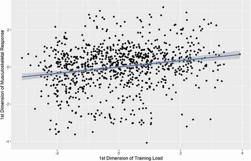
Figure 2 highlights the correlation between the latent variables of training load and musculoskeletal response for the first dimension for the group level analysis. The group level correlation (r value [95% confidence interval]) between the 1^st dimension latent variables of training load (X) and musculoskeletal response (Y) was r = 0.20 (0.14 to 0.27; p < 0.00001).

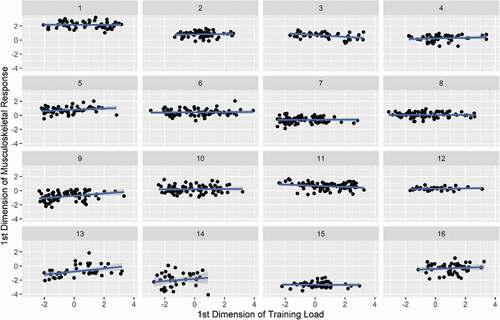
Figure 3 highlights the correlations between the latent variables of training load and musculoskeletal response for the 1^st dimension for each of the 16 individual players. The pooled repeated measures correlation (r value [95% confidence interval; p-value]) between the 1^st dimension latent variables of training load (X) and musculoskeletal response (Y) (Figure 2) was r = 0.06 (0.00 to 0.13; p = 0.47).

Figure 3. Scatterplots of the X (training load) and Y (musculoskeletal response) latent variables for the 1st dimension of the refined PLSCA model for each observation for each of the 16 individual players

Discussion

The primary aim was to utilise latent variable modelling (PLSCA) to (1) determine the relative importance of external load measurements to relate to multiple musculoskeletal responses measures and (2) calculate latent training load and musculoskeletal variables to identify the strength of relationship between the two on a group and individual level in elite rugby league players across three seasons. Although the total distance covered in the previous 2 and 3 days (EWMA) were identified as the most relative important training load measures, the strength of such relationships on both a group (r = 0.20) and individual player level (pooled r = 0.06) suggest a lack of relationship between the constructed latent training load and musculoskeletal response variables. Taken together, it would appear that common measures to represent the musculoskeletal response do not respond to changes in training load on a group or individual player level and so using such measures to make conclusions on an athletes fatigue response would be limited.

The current study is the first to report the relationship between total- and individualised-high-speed-distances and musculoskeletal responses in team sport athletes. The current study findings support previous studies that have used internal load measures of sRPE and identified a lack of relationship with changes in musculoskeletal response (Esmaeili et al., 2018; Lonie et al., 2020). Collectively, both current and previous findings suggest that either (1) total- and individualised-high-speed-distances are unable to provide an estimate of future musculoskeletal responses or (2) the musculoskeletal response measurements lack sensitivity to changes in training load (Esmaeili et al., 2018). In the current study, Figure 2 highlights the greater variability in training load across a longitudinal observation period than the musculoskeletal response. This is supported by the findings of Esmaeili et al. (2018) who reported small to moderate within-individual variability in weekly sit and reach (0.92 ± 0.14 cm), dorsiflexion lunge test (0.50 ± 0.08 cm) and adductor squeeze (7.8 ± 0.8%) across pre- and in-season periods within professional Australian Rules footballers. However, Lonie et al. (2020) reported significant changes in pooled adductor squeeze strength across pre-season, end of pre-season, mid-season, and post-season time points. Differences in the variability in musculoskeletal response between studies could be due to the different time periods in which the data were aggregated, with weekly (current study; Esmaeili et al., 2018) and seasonal (e.g. pre-season and in-season) (Lonie et al., 2020) time periods used. In addition, numerous studies have identified relationships with both external and internal training load measures and measurements of fatigue of other systems (e.g. cardiovascular, neuromuscular). For example, Oxendale et al. (2016) reported substantial relationships between the number of collisions during professional rugby league match play and changes in repeated plyometric push up performance (r = −0.48) whilst Williams et al. (2018) reported sRPE to explain a substantial amount of variability in changes in heart rate variability (r = 0.66) in elite rugby sevens players. Therefore, current and previous findings suggest that the stability in musculoskeletal screening measures over short time periods (i.e. daily and weekly) mean that these measures are unlikely to provide insight into the acute musculoskeletal recovery from the prescribed training load (i.e. as a measurement of the fatigue response). As such, the findings of current and previous research suggest practitioners utilising musculoskeletal measures for this reason should do so with caution and explore other measurements to support insight into this construct such as power or force-related variables derived from sprinting and jumping activity (Twist & Highton, 2013).

In the age of technology (Coutts, 2014), it can difficult for the applied sports scientist to balance the requirements of evaluating the multiple dimensions that comprise the training process yet also visualise multiple variables more simply to inform the decision makers of the training process (e.g. coaches) (Weaving et al., 2019). The current study is the first to provide an example of how PLSCA models can be implemented to represent and visualise the “composite” relationship between multiple independent and multiple dependent variables in a reduced number of dimensions via the latent variable approach (Figure 2). By conducting PLSCA, the saliences (Table 2) can be used in combination with the mean centred and standardised data to create latent variables (akin to principal component scores) (Weaving et al., 2019). For example, in the current study, a latent variable of training load was computed by multiplying the original mean centred and standardised data by the saliences ([0.73 × 2 day EWMA total distance] + [0.68 × 3 day EWMA total distance]) and replicated for the musculoskeletal response measures ([0.70 * S&R] + [0.08×DLT_LEFT] + [0.36×DLT_RIGHT] + [0.62 *AST]). Such saliences can be used in day-to-day practice to allow practitioners to provide a latent variable composite score of training load and fatigue response for each training day. When faced with datasets comprising multiple independent and dependent performance-related variables, such techniques can overcome issues of multicollinearity (Abdi & Williams, 2013; Weaving et al., 2019) and also reduce the requirement to produce multiple competing models which frequently occurs when adopting univariate approaches such as linear regression (i.e. one independent to one dependent variable) or multiple linear regression (i.e. multiple independent to one dependent variable). The issue of multiple comparisons centres on the increased likelihood of an inflated Type I error rate and should be considered when constructing dose–response relationships (Knudson & Lindsey, 2014). However, PLSCA can represent multiple co-linear dependent variables within a single analysis whilst attempting to minimise the loss of information (i.e. variance). Consequently, we have for the first time, demonstrated the use of this method to analyse and visualise complex dose–response relationships that are comprised of multiple, interrelated variables. Future research is needed to understand the usefulness of such approaches in other areas of the training process.

A limitation of the current study is the lack of quantification of the collision training load imposed onto the players. Substantial increases in energy expenditure (Costello et al., 2018) and markers of muscle damage (Oxendale et al., 2016; Naughton et al., 2018) are present following the addition of collisions (Costello et al., 2018; Naughton et al., 2018; Oxendale et al., 2016). Furthermore, we did not investigate the influence of certain locomotor movements (e.g. changes in speed; accelerations and decelerations) or individual player characteristics (e.g. changes in body mass, physical qualities) that are also likely to contribute or mediate the biomechanical/musculoskeletal load imposed onto players across a longitudinal period of time. Therefore, by not quantifying these aspects of training and competition training load or changes in player characteristics, we are likely not accounting for a substantial proportion of the internal training load imposed onto these athletes following training. Additionally, the current study did not test the 30–15_IFT and update the individualised high-speed thresholds during the in-season period. Collectively, these might explain the lack of significant relationships between any of the measured external load variables and musculoskeletal response for the individual players in the current study.

Conclusions

This study provides practitioners with a better understanding of the relationship between total distance, and individualised high-speed threshold distances, EWMA periods and common measurements used to represent musculoskeletal function on both a group- and individual-based level. Additionally, how latent variable models can help to analyse and visualise complex relationships between multiple independent and dependent variables. Our analysis demonstrates that on a group level, the 2–3 day EWMA of the total distance covered were most relatively important to explain the collective musculoskeletal fatigue response, as represented by adductor squeeze, sit and reach and left and right-leg ankle dorsiflexion tests. However, on both group and individual player level analyses, these training load variables had limited relationship to the collective musculoskeletal response. Taken together, it would appear that common measures to represent the musculoskeletal response do not respond to changes in training load and so using such measures to make conclusions on an athletes fatigue response would be limited.

Disclosure of potential conflicts of interest

No potential conflict of interest was reported by the authors.

References

- Abdi, H., & Williams, L. J. (2013). Partial least squares methods: Partial least squares correlation and partial least square regression. Methods in Molecular Biology (Clifton, N.J.), 930, 549–579. https://doi.org/https://doi.org/10.1007/978-1-62703-059-5_23
- Akenhead, R., & Nassis, G. P. (2016). Training load and player monitoring in high-level football: Current practice and perceptions. International Journal of Sports Physiology and Performance, 11(5), 587–593. https://doi.org/https://doi.org/10.1123/ijspp.2015-0331
- Bakdash, J. Z., & Marusich, L. R. (2017). Repeated measures correlation. Frontiers in Psychology, 8, 456. https://doi.org/https://doi.org/10.3389/fpsyg.2017.00456
- Banister, E. W., Calvert, T. W., Savage, M. V., & Bach, A. (1975). A system model of training for athletic performance. Australian Journal of Sports Medicine, 7, 170–176.
- Barker, M., & Rayens, W. (2003). Partial least squares for discrimination. Journal of Chemometrics, 17(3), 166–173. https://doi.org/https://doi.org/10.1002/cem.785
- Barr, M., Beaver, T., Turczyn, D., & Cornish, S. (2019). Validity and reliability of 15 Hz global positioning system units for assessing the activity profiles of university football players. Journal of Strength and Conditioning Research, 33(5), 1371–1379. https://doi.org/https://doi.org/10.1519/JSC.0000000000002076
- Bennell, K., Talbot, R., Wajswelner, H., Techovanich, W., Kelly, D., & Hall, A. (1998). Intra-rater and inter-rater reliability of a weight-bearing lunge measure of ankle dorsiflexion. Australian Journal of Physiotherapy, 44(3), 175–180. https://doi.org/https://doi.org/10.1016/S0004-9514(14)60377-9
- Costello, N., Deighton, K., Preston, T., Matu, J., Rowe, J., Sawczuk, T., Halkier, M., Read, D. B., Weaving, D., & Jones, B. (2018). Collision activity during training increases total energy expenditure measured via doubly labelled water. European Journal of Applied Physiology, 118(6), 1169–1177. https://doi.org/https://doi.org/10.1007/s00421-018-3846-7
- Coutts, A. J. (2014). In the age of technology, Occam’s Razor still applies. International Journal of Sports Physiology and Performance, 9(5), 741. https://doi.org/https://doi.org/10.1123/ijspp.2014-0353
- Esmaeili, A., Stewart, A. M., Hopkins, W. G., Elias, G. P., Lazarus, B. H., Rowell, A. E., & Aughey, R. J. (2018). Normal variability of weekly musculoskeletal screening scores and the influence of training load across an Australian football league season. Frontiers in Physiology, 9, 144. https://doi.org/https://doi.org/10.3389/fphys.2018.00144
- Gabbe, B. (2004). Reliability of common lower extremity musculoskeletal screening tests. Physical Therapy in Sport, 5(2), 90–97. https://doi.org/https://doi.org/10.1016/S1466-853X(04)00022-7
- Hodgson, L., Hignett, T., & Edwards, K. (2015). Normative adductor squeeze tests scores in rugby. Physical Therapy in Sport, 16(2), 93–97. https://doi.org/https://doi.org/10.1016/j.ptsp.2014.08.010
- Impellizzeri, F. M., Rampinini, E., & Marcora, S. M. (2005). Physiological assessment of aerobic training in soccer. Journal of Sports Sciences, 23(6), 583–592. https://doi.org/https://doi.org/10.1080/02640410400021278
- Impellizzeri, F.M., Marcora, S.M. & Coutts, A.J. (2019). Internal and external training load: 15 years on. International Journal of Sports Physiology and Performance, 14(2), pp. 270–273.
- Kiely, J. (2018). Periodisation theory: confronting an inconvenient truth. Sports Medicine,48(4), 753–764.
- Knudson, D. V., & Lindsey, C. (2014). Type I and type II errors in correlations of various sample sizes. Comprehensive Psychology, 3, 1. https://doi.org/https://doi.org/10.2466/03.CP.3.1
- Krishnan, A., Williams, L. J., McIntosh, A. R., & Abdi, H. (2011). Partial Least Squares (PLS) methods for neuroimaging: A tutorial and review. Neuroimage, 56(2), 455–475. https://doi.org/https://doi.org/10.1016/j.neuroimage.2010.07.034
- Liquet, B., Le, Cao, KA., Hocini, H. & Thiebaut, R. (2012). A novel approach for biomarker selection and the integration of repeated measures experiments from two assays. BMC Bioinformatics, 13, 325. https://doi.org/https://doi.org/10.1186/1471-2105-13-325
- Lonie, T. A., Brade, C. J., Finucane, M. E., Jacques, A., & Grisbrook, T. L. (2020). Hip adduction and abduction strength and adduction-to-abduction ratio changes across an Australian Football League season. Journal of Science and Medicine in Sport, 23(1), 2–6. https://doi.org/https://doi.org/10.1016/j.jsams.2019.08.002
- MacInnis, M. J., & Gibala, M. J. (2017). Physiological adaptations to interval training and the role of exercise intensity. The Journal of Physiology, 595(9), 2915–2930. https://doi.org/https://doi.org/10.1113/JP273196
- Malone, JJ., Lovell, R., Varley, MC. & Coutts, A.J. (2017). Unpacking the black box: applications and considerations for using GPS devices in sport. International Journal of Sports Physiology and Performance,12(Suppl 2), S218–S226.
- McIntosh, A. R., & Misic, B. (2013). Multivariate statistical analyses for neuroimaging data. Annual Review of Psychology, 64(1), 499–525. https://doi.org/https://doi.org/10.1146/annurev-psych-113011-143804
- McLaren, S. J., Smith, A., Spears, I. R., & Weston, M. (2017). A detailed quantification of differential ratings of perceived exertion during team-sport training. Journal of Science and Medicine in Sport, 20(3), 290–295. https://doi.org/https://doi.org/10.1016/j.jsams.2016.06.011
- Naughton, M., Miller, J., & Slater, G. J. (2018). Impact-induced muscle damage: Performance implications in response to a novel collision simulator and associated timeline of recovery. Journal Of Science And Medicine In Sport / Sports Medicine Australia, 17(3), 417–425. https://doi.org/https://doi.org/10.1123/ijspp.2017-0268
- Oxendale, C. L., Twist, C., Daniels, M., & Highton, J. (2016). The relationship between match-play characteristics of elite rugby league and indirect markers of muscle damage. International Journal of Sports Physiology and Performance, 1(4), 515–521. https://doi.org/https://doi.org/10.1123/ijspp.2015-0406
- Oxendale, CL., Twist, C., Daniels, M. & Highton, J. (2016). The relationship between match-play characteristics of elite rugby league and indirect markers of muscle damage. International Journal of Sports Physiology and Performance,11(4), pp. 515–521. https://doi.org/https://doi.org/10.1123/ijspp.2015-0406
- Roe, G. A., Phibbs, P. J., Till, K., Jones, B. L., Read, D. B., Weakley, J. J., & Darrall-Jones, J. D. (2016). Changes in adductor strength after competition in academy rugby union players. Journal of Strength and Conditioning Research, 30(2), 344. https://doi.org/https://doi.org/10.1519/JSC.0000000000001024
- Ryan, S., Kempton, T., Impellizzeri, F. M., & Coutts, A. J. (2020). Training monitoring in professional Australian football: Theoretical basis and recommendations for coaches and scientists. Science and Medicine in Football, 4(1), 52–58. https://doi.org/https://doi.org/10.1080/24733938.2019.1641212
- Scott, T., & Kelly, V. (2017). Normative values, longitudinal trends and usefulness of adductor dynamometry to detect fatigue in professional rugby league players. The Journal of Australian Strength and Conditioning, 25(6), 44.
- Scott, T. J., McLaren, S. J., Caia, J., & Kelly, V. G. (2018). The reliability and usefulness of an individualised submaximal shuttle run test in elite rugby league players. Science and Medicine in Football, 2(3), 184–190. https://doi.org/https://doi.org/10.1080/24733938.2018.1448937
- Soligard, T., Schwellnus, M., Alonso, J.-M., Bahr, R., Clarsen, B., Dijkstra, H. P., Gabbett, T., Gleeson, M., Hägglund, M., Hutchinson, M. R., Janse van Rensburg, C., Khan, K. M., Meeusen, R., Orchard, J. W., Pluim, B. M., Raftery, M., Budgett, R., & Engebretsen, L. (2016). How much is too much? (Part 1) International Olympic Committee consensus statement on load in sport and risk of injury. British Journal of Sports Medicine, 50(17), 1030–1041. https://doi.org/https://doi.org/10.1136/bjsports-2016-096581
- Tessaro, E., & Williams, J. H. (2018). Validity and reliability of a 15 Hz GPS device for court-based sports movements. Sport Performance & Science Reports, 29, 1–4.
- Thorpe, R. T., Strudwick, A. J., Buchheit, M., Atkinson, G., Drust, B., & Gregson, W. (2017). The influence of changes in acute training load on daily sensitivity of morning-measured fatigue variables in elite soccer players. International Journal of Sports Physiology and Performance, 12(Suppl s2), SS2107–389 S2113. https://doi.org/https://doi.org/10.1123/ijspp.2016-0433
- Till, K., Jones, B., Cobley, S., Morley, D., O’Hara, J., Chapman, C., Cooke, C., Beggs, C. B., & Sampaio, J. (2016). Identifying talent in youth sport: A novel methodology using higher-dimensional analysis. PLoS One, 11(5), e0155047. https://doi.org/https://doi.org/10.1371/journal.pone.0155047
- Twist, C., & Highton, J. (2013). Monitoring fatigue and recovery in rugby league players. International Journal of Sports Physiology and Performance, 8(5), 467–474. https://doi.org/https://doi.org/10.1123/ijspp.8.5.467
- Vanrenterghem, J., Nedergaard, N. J., Robinson, M. A., & Drust, B. (2017). Training load monitoring in team sports: A novel framework separating physiological and biomechanical load-adaptation pathways. Sports Medicine, 47(11), 2135–2142. https://doi.org/https://doi.org/10.1007/s40279-017-0714-2
- Veugelers, K. R., Naughton, G. A., Duncan, C. S., Burgess, D. J., & Graham, S. R. (2016). Validity and reliability of a submaximal intermittent running test in elite Australian football players. Journal of Strength and Conditioning Research, 30(12), 3347–3353. https://doi.org/https://doi.org/10.1519/JSC.0000000000001441
- Weaving, D., Jones, B., Ireton, M., Whitehead, S., Till, K., Beggs, C. B., & Connaboy, C. (2019). Overcoming the problem of multicollinearity in sports performance data: A novel application of partial least squares correlation analysis. PLoS One, 14(2), e0211776. https://doi.org/https://doi.org/10.1371/journal.pone.0211776
- Weaving, D., Jones, B., Till, K., Marshall, P., Earle, K., & Abt, G. (2020). Quantifying the external and internal loads of professional rugby league training modes: Consideration for concurrent field-based training prescription. Journal of Strength and Conditioning Research, 34(12), 3514-3522. https://doi.org/https://doi.org/10.1519/JSC.0000000000002242
- Williams, S., West, S., Cross, M. J., & Stokes, K. A. (2017). Better way to determine the acute:chronic workload ratio? British Journal of Sports Medicine, 51(3), 209–210. https://doi.org/https://doi.org/10.1136/bjsports-2016-096589
- Williams, S., West, S., Howells, D., Kempt, S. P. T., Flatt, A. A., & Stokes, K. (2018). Modelling the HRV response to training loads in elite rugby sevens players. Journal of Sports Science & Medicine, 17(3), 402–408.