Drift correction for accurate PRF-shift MR thermometry during mild hyperthermia treatments with MR-HIFU

Abstract

There is growing interest in performing hyperthermia treatments with clinical magnetic resonance imaging-guided high-intensity focused ultrasound (MR-HIFU) therapy systems designed for tissue ablation. During hyperthermia treatment, however, due to the narrow therapeutic window (41–45 °C), careful evaluation of the accuracy of proton resonant frequency (PRF) shift MR thermometry for these types of exposures is required.

Purpose: The purpose of this study was to evaluate the accuracy of MR thermometry using a clinical MR-HIFU system equipped with a hyperthermia treatment algorithm.

Methods: Mild heating was performed in a tissue-mimicking phantom with implanted temperature sensors using the clinical MR-HIFU system. The influence of image-acquisition settings and post-acquisition correction algorithms on the accuracy of temperature measurements was investigated. The ability to achieve uniform heating for up to 40 min was evaluated in rabbit experiments.

Results: Automatic centre-frequency adjustments prior to image-acquisition corrected the image-shifts in the order of 0.1 mm/min. Zero- and first-order phase variations were observed over time, supporting the use of a combined drift correction algorithm. The temperature accuracy achieved using both centre-frequency adjustment and the combined drift correction algorithm was 0.57° ± 0.58 °C in the heated region and 0.54° ± 0.42 °C in the unheated region.

Conclusion: Accurate temperature monitoring of hyperthermia exposures using PRF shift MR thermometry is possible through careful implementation of image-acquisition settings and drift correction algorithms. For the evaluated clinical MR-HIFU system, centre-frequency adjustment eliminated image shifts, and a combined drift correction algorithm achieved temperature measurements with an acceptable accuracy for monitoring and controlling hyperthermia exposures.

Keywords:

• Mild hyperthermia
• MR-HIFU
• PRF-shift MR thermometry
• phase drift

Introduction

High-intensity focused ultrasound guided by magnetic resonance temperature mapping (MR-HIFU) is a non-invasive method for thermal therapy [1–3] which can achieve precise localisation and control of heating within the body for the application of mild hyperthermia or tissue ablation. Clinical MR-HIFU systems have been developed for treatment of uterine fibroids [4–6], bone metastases [7–9], essential tremor [10,11], localised breast cancer [12–14], and prostate cancer [15–18]. These systems are designed to generate irreversible thermal coagulation in the target tissue as the therapeutic end point. During the delivery of ultrasound energy, MR thermometry is used to monitor (and in some cases control) the level of heating at the target site and surrounding sensitive tissues during a series of short exposures. MR-HIFU systems are also being developed or adapted to perform mild hyperthermia [19–23]. For this application, the aim is to heat a larger tissue volume in the range of 41–45 °C for durations ranging from a few minutes up to an hour. This extended period of mild heating can be cytotoxic on its own [24], can sensitise tissues to radiation [25,26] or chemotherapy [27] and can also be used as a means of triggering the local release of drugs from temperature-sensitive carriers [28–34].

From a technical perspective, delivery of mild hyperthermia in the body is very challenging. Since temperatures within a very narrow window must be maintained for up to 1 h, accurate temperature feedback from the heated volume is critical to compensate for changes in the heating pattern arising from variations in blood flow and energy absorption that occur during treatment. The proton resonant frequency shift (PRF shift) [35,36] method of MR thermometry is commonly used to measure tissue temperature during ablative MR-HIFU treatments. Using clinical imaging systems, temperature precision in the order of 1–2 °C is achieved in various tissue types with a temporal resolution of a few seconds, a spatial resolution of a few mm [37–40], in multiple image planes providing volumetric feedback in and around the target volume. These sequences are typically acquired for less than 1–2 min during individual ablative exposures [4]. In contrast, for mild hyperthermia an accuracy of <1 °C is desirable since the therapeutic window is so narrow, and the precision as well as the stability of the measurement must be maintained for durations ranging from 10 min to 1 h. Aside from subject motion, important considerations are the image shift caused by gradual fluctuations of the centre frequency of the MR scanner due to environmental changes (magnetic field drift), and dynamic temporal and spatial fluctuations of magnetic field due to heating of magnet components during scanning. These magnetic field fluctuations cause errors in MR temperature measurements which can accumulate over time.

The objective of this study was to evaluate the accuracy of PRF shift MR thermometry over the time periods required for mild hyperthermia, and to develop appropriate strategies for accurate tissue temperature measurements using this method with a clinical MR-HIFU system. A series of experiments in phantoms are described that evaluate the influence of environmental parameters and correction strategies on MR temperature measurement accuracy. Proposed strategy is evaluated in preclinical studies in a rabbit model during long-duration mild hyperthermia exposures (10–40 min).

PRF shift MR thermometry and drift correction strategies

In PRF shift MR thermometry, temperature maps are calculated from changes in the phase of gradient echo images caused by the temperature-dependent change in resonance frequency. In a simple scenario, temporal changes in phase due to heating are separated from static spatial phase variations due to B₀ inhomogeneities that exist before heating, by subtracting a reference image acquired before heating started. This results in the calculation of a change in temperature Δ T (1) where ø (T₀) is the current phase map, ø (T₀) is the reference phase map, γ is the gyromagnetic ratio, α is the temperature sensitivity of the PRF shift, B₀ is the main magnetic field strength and TE is the echo time. When temperature mapping data is acquired in multiple image planes, the set of images from all planes acquired at one time step is referred to as a dynamic.

However, there are multiple sources of temperature-independent phase drift that can violate the assumption that only temperature changes account for the phase changes between different time points or spatial locations. These include gradient heating of passive shims [41,42], variations in electrical conductivity [43], temperature-dependent changes in magnetic susceptibility [35,44], and time-varying magnetic susceptibility disturbances caused by devices [45,46] or patient motion [47–49]. Others have shown that these sources can result in typical rates of B₀ drift ranging from 0.01 to 0.06 ppm/min [50,51]. When converted to temperature using Equation 1(1) with typical parameters of α  = 0.0094 ppm/°C, B₀ = 3 T, and TE = 16 ms, the resulting phase errors are 0.1 to 0.8 rad/min, or an apparent temperature change of up to 7 °C/min. These errors accumulate further over several minutes of scanning, necessitating the use of drift correction algorithms to recover the true temperature change. Large phase changes can be caused by patient motion (rapid local changes of more than 2.5 ppm [52]), which can produce a phase error of more than 32 rad (or a temperature change of more than 265 °C). However, only small and gradual changes induced by the phase drift will be covered in this study since these are more difficult to detect and separate from the heating occurring due to hyperthermia.

Drift correction can be applied either before image acquisition, before reconstruction [53], or to the reconstructed image [54]. While many variations and potential combinations exist for drift correction, a primary motivation in evaluating the combinations described in this study was for the purpose of validating the accuracy of an algorithm implemented in research software on the Philips Sonalleve^® MR-HIFU system for performing mild hyperthermia treatments with a Philips 3 T MR scanner (Ingenia, Philips Healthcare, Vantaa, Finland).

Prospective correction

In addition to errors in temperature measurement, the phase offsets in k-space data translate into spatial shifts in the images after performing the inverse Fourier transform. A prospective method to correct for this spatial shift artefact before reconstruction drift correction involves measuring and adjusting the centre frequency before each scan [55]. This type of correction is referred to as F₀ dynamic stabilisation (DS) on the MR scanner utilised in this study (Ingenia 3T, Philips Healthcare). This feature is user-selectable for dynamic acquisitions on 3T Philips MR scanners, but might require customised sequence development on other magnet platforms. With DS enabled, phase shift with respect to the initial resonance frequency is calculated from a small flip-angle, 3-echo acquisition inserted at the beginning of each dynamic [56]. This method also has the effect of counteracting global drift of the B₀ field. Here, the impact of DS on the accuracy of MR thermometry is evaluated.

Retrospective correction

In clinical MR thermometry, phase drift correction is most often done in image space after reconstruction of magnitude and phase images of each dynamic in a time series [37,38,57]. For MR-HIFU therapy, reconstruction, correction, and display all need to be done in real time. Phase drift can be measured within an image region of interest (ROI) that remains at a fixed temperature [58]. The simplest correction to apply across the image is a subtraction of the average change measured in this ROI. This is referred to as a zero-order drift correction (DC), and is usually sufficient for the short-duration heating encountered in MR-HIFU ablation. However, over a longer time period of minutes, additional spatially varying changes in the background phase accumulate across the image. These components of the phase drift can be described by first and second order polynomial functions, fitted over large or multiple ROIs [50,54,59]. Fitting of background phase can be performed separately for the 2D data from each image, or on the combined 3D data from all images acquired in one dynamic.

Description of proposed drift correction strategy

The drift correction strategy evaluated in this study includes two forms of prospective drift correction (DS and pre-scan imaging), followed by a retrospective drift correction algorithm applied on the reconstructed images. DS works in the same way described in the previous section. Pre-scan imaging involves a 10-min acquisition of the temperature mapping sequence immediately prior to the MR thermometry experiment, intended to bring the magnet hardware to a thermal steady state. The retrospective drift correction algorithm uses a slice-by-slice DC correction of changes in the main magnetic field strength, combined with a 3D first-order correction of changes in the spatial distribution of the main magnetic field (referred to as DC+3D).

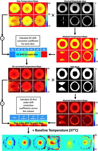
The DC+3D drift correction algorithm is shown graphically in Figure 1. The processing pipeline for an individual dynamic can be described as follows. 1) Exclude all voxels within the expected heating area using the masked magnitude map to generate the raw masked temperature maps. 2) Calculate a slice-by-slice DC drift estimate (S1–S6) for each slice and generate the DC-corrected temperature maps. 3) Combine the DC-corrected temperature maps with the SNR mask excluding all voxels with temperature uncertainty >3 °C. 4) Perform a least squares fit on the masked DC-corrected temperature maps over the voxels from all slices of the current dynamic, generating four correction coefficients: one zero-order coefficient and three first-order coefficients along different directions. Apply these coefficients onto each slice to get the 3D first-order temperature error maps. 5) Apply the first-order temperature error map and the DC drift estimate on to the baseline temperature, generating the final temperature maps used for display and feedback control.

Figure 1. Processing pipeline for the retrospective drift correction algorithm evaluated in this study. The main algorithm comprised of a DC drift correction and a 3D first-order drift correction.

Methods and materials

First, the influence of magnet temperature was quantified to assess the importance of applying drift correction during long-duration MR thermometry. Subsequently, proposed drift correction strategies were evaluated individually and in combination, and validated against implanted temperature sensors. Finally, the stability of drift correction was evaluated in vivo. Detailed scanner settings (ACQ1, ACQ2, ACQ3) used for different image acquisitions are summarised in Table 1.

Table 1. Acquisition information of different scans applied in this study. Three sequences (referred as ACQ1, ACQ2, and ACQ3) in total were performed based on the experiment requirement. TE and TR represent echo time and repetition time, respectively.

	Sequence type	TE (ms)	TR (ms)	Resolution	Field of view (cm)	Voxel size (mm)	Fat suppression	Time per dynamic	Number of slice
1	FFE-EPI, EPI factor =11	16	25.18	192 × 192	40 × 40	2.1 × 2.1 × 7.0	ProSet	2.6 s	6
2	FFE	16	22.74	192 × 192	40 × 40	2.1 × 2.1 × 7.0	None	6.7 s	2
3	FFE-EPI, EPI factor =9	16	31	160 × 160	24 × 24	1.5 × 1.5 × 5.0	None	3.9 s	6

Influence of magnet temperature on phase drift

To evaluate the influence that heating of magnet hardware during scanning has on background phase drift [42], phase images were acquired with two pulse sequences having different gradient duty cycles, and thus hardware heating rates, while simultaneously measuring the temperature of the inner magnet bore and the imaged sample. In this experiment a cylindrical phantom (MR-HIFU QA Phantom, Philips Healthcare, Vantaa, Finland) was imaged in a 3-T MR scanner (Ingenia, Philips Healthcare). Two fibre-optic probes (T1, Neoptix, Canada) were taped to the inner surface of the bore, and two fibre-optic probes were inserted into the phantom, recording the actual temperature during the scan with a temporal resolution of 1 s. Scanning with a segmented fast field echo-echo planar imaging sequence (ACQ1) was performed for 60 min, and temperature monitoring continued after scanning ended until the bore temperature dropped to baseline. A similar measurement was made while scanning with a conventional spoiled fast field echo sequence (ACQ2), which has a lower gradient duty cycle and is expected to cause less heating to the magnet bore. In both cases, the patient ventilation fan of the MRI was set at the same level. There was no scanning performed in the 2 h prior to this measurement, and the magnet was in a stable thermal configuration. For both imaging acquisitions, the mean phases in an ROI located around the two probes were measured over time to quantify phase drift within the assumed target region for treatment.

Influence of pre-scan imaging and F₀ dynamic stabilisation on phase drift

The effects of the two prospective drift compensation approaches on phase drift were evaluated based on their influence over the coefficients of a 3D first-order fit to the background phase. Phase images were acquired using a 3 T MR scanner (Ingenia) with an integrated MR-HIFU system (Sonalleve V2, Philips Healthcare). Temperature maps were processed with prototype software on the MR-HIFU system that uses an algorithm similar to the 3D first-order drift correction algorithm described in the previous section. MR images of a cylindrical phantom (MR-HIFU QA Phantom, Philips Healthcare) were acquired using the five-channel coil array of the MR-HIFU system. After B1 calibration and a 3D T1-weighted planning scan, temperature maps (ACQ1) were acquired for 60 min with the HIFU transducer disabled (no heating).

Influence of F₀ dynamic stabilisation on image displacement

Beyond erroneous phase values within a voxel, phase drift causes shifts in reconstructed images if present in the k-space data. If the amount of image shift is in the order of a voxel or greater it will cause errors in the phase subtraction used for PRF-shift MR thermometry. DS can correct this error due to its operation on k-space data directly. To quantify this displacement, the segmented echo-planar imaging (EPI) temperature mapping sequence (ACQ1) was acquired for 30 min either with or without DS. Image shift was estimated based on the frequency content of reconstructed magnitude images. The central frequency displacement between each dynamic and the reference (the first dynamic) was calculated from the fast Fourier transform (FFT) of the magnitude images. The image shift was then retrieved by inverse FFT of the central frequency displacement. Image shift along the phase/frequency encoding direction was measured with or without DS.

Interaction between slice-by-slice DC correction and 3D first-order drift correction coefficients

To evaluate the influence of slice-by-slice DC drift correction on the 3D first-order drift correction coefficients, the data acquired with DS enabled and pre-scan imaging were reprocessed with and without DC drift correction. The DC correction was applied to the raw temperature data from each image slice, prior to fitting the 3D drift correction coefficients. It is expected that the slice-by-slice correction would reduce temporal variations between dynamics and individual slices of each dynamic.

Validation tests of individual and combined drift correction strategies

A series of validation tests were performed to evaluate the accuracy of MR thermometry under eight different conditions. The evaluations were primarily categorised into two groups based on the application of prospective drift correction. Pre-scan imaging was performed for 10 min for all cases, while DS was either turned on (n = 6) or off (n = 3). Four conditions were evaluated under each group for different retrospective correction methods: 1) raw temperature measurements acquired without applying retrospective drift correction, noted as ‘no correction’, 2) temperature measurements corrected with slice-by-slice DC drift correction, noted as ‘DC only’, 3) temperature measurements corrected with 3D first-order correction, noted as ‘3D only’, 4) temperature measurements corrected with proposed retrospective drift correction algorithm, noted as ‘DC+3D’. For each drift correction approach, MR temperature measurements acquired during MR-HIFU heating of a gel phantom were compared against temperatures measured using implanted fibre-optic sensors.

A gellan gum tissue-mimicking phantom (radius = 3.75 cm, height = 8 cm) was used in this experiment [60]. Two fibre-optic temperature probes were inserted into the phantom to measure the local temperature in the heated region (Probe 1) and in an unheated location (Probe 2) during the heating experiment. The phantom was placed on the clinical HIFU tabletop, fitted on a customised adaptor filled with degassed water. A set of T1-weighted images were acquired for treatment planning (Figures 2(A) and 2(B)), and used to define an 8-mm diameter circular target region centred on Probe 1. A ring of 16 focal point locations along the circumference of the target region (Figure 2(C)) was sonicated to achieve a zone of uniform heating around Probe 1, while reducing temperature measurement artefacts caused by ultrasound energy directly impinging on the probes [61]. The ultrasound transducer was driven at 1.2 MHz, with 10 W output power for 600 s.

Figure 2. T1-weighted images acquired along (A) and across (B) the ultrasound beam. Two fibre-optic temperature probes were used to validate MR thermometry during MR-HIFU hyperthermia exposures in a phantom. The dashed line in (A) depicts the centre of the plane where MR thermometry was performed during heating. The locations of two temperature probes are shown in (B). Zoomed-in view of the dashed square region in (B) is shown in (C), with the precise location of heating. The ultrasound beam was rapidly scanned along an 8-mm circular trajectory resulting in a uniform region of heating around probe 1.

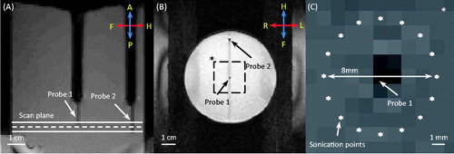
During the sonication, temperature maps were acquired using a segmented EPI sequence (ACQ3) with 10 min of scanner pre-heating, and using a PRF shift temperature sensitivity, α, of −0.0094 ppm/°C. Each sonication lasted for 10 min, and scanning continued for a further 10 min to track the temperature in the gel as it cooled. For each probe, the mean MR temperature measurement within a 6 mm diameter circular ROI around the probe was compared with the probe readings. The reported error was calculated as the mean difference between corresponding MR and fibre-optic temperature measurements.

Although the focus did not hit the fibre-optic probe directly, the ultrasound field at the probe location was not zero. A constant 1.4 °C offset for the centre probe was observed, which was related to viscous heating between the optical fibre’s plastic coating and the surrounding gel when the ultrasound power was turned on and off [61]. This offset was subtracted from all readings on the centre probe made during the sonication. The reference probe did not require correction as it was well away from the path of the ultrasound beam.

In-vivo evaluation of MR thermometry during long-duration MR-HIFU hyperthermia

To demonstrate the performance of MR thermometry derived with the proposed strategies during MR-HIFU mild hyperthermia treatment, animal experiments were conducted in a rabbit model with different heating durations (10–40 min). Female 3–4-kg New Zealand white rabbits (n = 16) with VX2 tumours were used in this study. All procedures were approved by the Universty of Texas Southwestern Institutional Animal Care and Use Committee under protocol APN 2013-0117. Briefly, animals were intubated and anaesthetised with a mixture of 2–3.5% isoflurane and 1–2 L/min of 100% oxygen. An intravenous catheter was placed in the ear vein for contrast agent administration. A pulse oximeter was attached to the animal’s tongue to monitor heart rate and oxygen saturation, and a rectal temperature probe (T1, Neoptix, Quebec, Canada) was used to record the core body temperature throughout the experiment. Hair over the animals’ thighs was removed using an electric trimmer and depilatory cream (VEET sensitive formula, Reckitt Benckiser, Parsippany, NJ, USA) to enable ultrasound transmission into the muscle. After preparation the animal was transferred to the clinical MR-HIFU tabletop, positioned on its side with its thigh placed over the ultrasound window. A custom HIFU adaptor consisting of a temperature-controlled water tank, a gel pad holder and a supporting platform was developed and designed to position the animal at an appropriate height and to maintain its body temperature over the heating period (Figure 3(A)). Ultrasound gel was applied on the thigh facing the acoustic window as well as the area in between the hind legs to avoid undesired reflections of the ultrasound beam. Two fibre-optic probes were placed in the water tank and on the skin to monitor the reference temperature of the animals.

Figure 3. (A) T1-weighted image along the ultrasound beam axis shows the experimental set-up for performing hyperthermia in a rabbit model. A gel pad and a water tank were placed on top of the acoustic window of the clinical MR-HIFU system to elevate the animal to the location of the ultrasound focus. The conical water tank also maintained the body temperature of the animals. (B) T2-weighted image transverse to the beam axis (along the dashed line in A) shows the VX2 tumour and the location of heating. (C) The spatial temperature distribution measured midway during treatment shows localised heating within the target area, well maintained in the desired range of 41–43 °C.

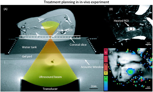
All hyperthermia experiments were performed using the MR scanner and MR-HIFU system described earlier. Temperature maps were acquired with 10 min of pre-scan imaging and DS turned on. DC+3D drift correction were applied to temperature measurements by modified research software. After a B1 calibration scan, 3D T1-weighted images were acquired to locate the target region for treatment planning (Figure 3(A)). A 10-mm diameter hyperthermia treatment cell was placed in a targeted region within the thigh. The 10-mm hyperthermia treatment cell is defined as a region consisting of electronically targeted sonication points at locations distributed over circular trajectories of 4 and 8 mm diameter. The location of the treatment cell was adjusted to ensure that the ultrasound beam would not interfere with bones or air interfaces to avoid ultrasound reflections or unexpected subject motion during therapy.

During hyperthermia treatment six images were acquired (ACQ1) for each dynamic scan: one slice along the ultrasound beam, three slices across the beam placed at the centre of the treatment cell, and two more slices to provide information from the near and far field across the ultrasound beam. The ultrasound frequency was 1.2 MHz, and the output power was 60 W. The temperature within the targeted region was maintained within 41–43 °C by the hyperthermia software using a prototype temperature feedback control algorithm based on previously described techniques [23,62,63]. Upon the completion of the sonication, an additional 10 min of imaging was included to monitor the tissue cooling.

The in vivo performance of the drift correction approach and hyperthermia feedback control was evaluated based on the temperature within the 10-mm diameter target region on the central slice across the ultrasound focus. The mean T90 (referring to the value lower than 90% of all temperature measurements) and T10 (referring to the value lower than 10% of all temperature measurements) in this ROI were calculated for each dynamic from the time the target region first reached the desired temperature range (41–43 °C) until the end of the sonication. The temporal stability of heating was summarised by the standard deviation of the target region mean, T90 and T10 across dynamics.

Results

Influence of magnet temperature on phase drift

Figure 4(A) shows the temperature measured on the inner surface of the magnet bore, and inside an imaged phantom during a 60-min temperature mapping scan using either a segmented EPI (ACQ1) or a conventional fast field echo (FFE) sequence (ACQ2). In both experiments the bore temperature curve was generated by averaging the readings from two probes taped on the inner bore. For the EPI sequence the bore temperature increased 5.3 °C (23.1° to 28.4 °C) over a period of approximately 60 min and started to reach a steady state. For the FFE sequence no significant temperature change was observed from the scanner bore. A minor temperature drop of 0.4 °C was observed due to the fan cooling. In both experiments the room temperature change was less than 0.5 °C.

Figure 4. Scanner temperature and phase change under different thermometry sequence. (A) Temperature of the inner bore of the MRI increased at different rates during scanning depending on the gradient duty cycle of the sequence: echo-planar (EPI, upper curve) versus fast field echo (FFE, lower curve). The scan parameter and fan setting in the MR console were kept the same for two sequences. (B) Phase measurements acquired with MR thermometry (red and blue increasing curves) in an unheated phantom during scanning shows a monotonic change in phase. No significant temperature change was observed in the phantom (green and pink flat curves). The rate of change appears to be related to the gradient duty cycle and magnet heating.

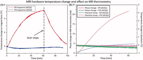
The phase drift observed with MR thermometry was higher for the EPI scan, which has a higher gradient duty cycle (Figure 4(B)). In the case of the conventional FFE sequence the phase change around the fibre-optic probes in the unheated phantom was averaged to be 4.5 rad (apparent temperature change of 37.2 °C from baseline), whereas it was 22.5 rad (apparent temperature change of 186.0 °C) for the EPI sequence. The real temperature of the phantom measured using two embedded fibre-optic probes showed no significant temperature change during the scan for both sequences.

By placing the fibre-optic probes on the inner surface of the bore, temperature measurements were made immediately adjacent to the transmit/receive body coil, and 1–2 cm away from the passive shims incorporated into the system. Temperature elevations measured using the probe during scanning are therefore likely to be related to heating of scanner components during heavy gradient use, but may also be partially affected by changes in air temperature in the imaging suite.

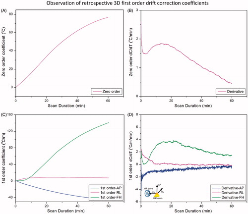
Observation of 3D first-order drift correction coefficients

Figure 5 shows an example of the drift correction coefficients calculated by the 3D first-order polynomial fit during scanning of an unheated phantom. At each dynamic the fit coefficients were calculated based on all slices in one dynamic. All curves were averaged with a sliding temporal window of 100 points to eliminate high frequency noise which obscured visualisation of the rate of change of these curves. The zero-order coefficients (Figure 5(A)) changed by approximately 77 °C over 60 min, corresponding to a phase drift of 3.1 rad. The temporal derivative of the zero-order coefficients (Figure 5(B)) shows variations in the first 10 min, which stabilise for longer scan times. The three first-order coefficients (Figure 5(C)) show a consistent change over time, with the coefficient in the foot–head (FH) direction (along the bore) being the largest component. The temporal derivatives of these coefficients (Figure 5(D)) also depict the greatest temporal variations in the first 10–20 min of scanning, followed by more consistent changes for longer scan times. After 60 min, the linear change in temperature across the image field of view (40 × 40 cm, ACQ1) in the FH direction was approximately 52 °C. Assuming a heated region of 3–4 cm, this would correspond to an error of up to 5 °C across this area, which requires correction for accurate hyperthermia.

Figure 5. Zero- and first-order correction coefficients across all slices acquired in 3D first-order drift correction. (A) Zero-order coefficients over 60 min of scanning for an unheated phantom in the magnet. (B) The rate of change of the zero-order coefficient ranges from 1–2 °C/min over the first 30 min, with greater temporal variation over the first 10–15 min. (C) First-order drift correction coefficients (in plane and through plane) over 60 min for the same unheated phantom in the magnet. (D) The rate of change of the first-order coefficients also depicts more temporal variation in the first 10–15 min followed by steady monotonic variations.

Influence of pre-scan imaging and F₀ dynamic stabilisation on phase drift

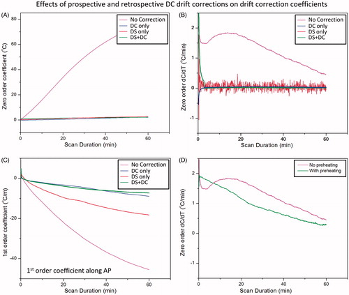
Figure 6 shows the effect of DS and 10 min of pre-scan imaging on both the magnitude and rate of change of the drift correction coefficients calculated using the 3D first-order polynomial fit. Not surprisingly, the zero-order coefficients were virtually eliminated after DS was enabled (Figure 6(A), red, flat curve). The rate of change was essentially zero as well (Figure 6(B), red, noisy flat curve), although this estimate of zero-order coefficients fluctuates more (temporal standard deviation 0.14 °C, red versus 0.01 °C, pink). One explanation for the increased variability might be due to the fact that DS compensates for the inaccurate estimation of F₀ acquired with only a few echoes, in a very short time, achieving a precision of approximately ±1 Hz, corresponding to a temperature precision of ±0.8 °C. Also, a single correction is used for all six slices of a dynamic. These factors result in a less accurate measurement of centre frequency compared to the slice-specific DC correction based on the average of a full image acquisition. Enabling DS also reduced the magnitude of the first-order coefficient along the anterior-posterior (AP) direction (Figure 6(C) red, middle curve). Performing a 10-min pre-scan imaging to ‘pre-heat’ the scanner eliminated the early temporal variations observed in the zero-order coefficients, as shown in Figure 6(D). These results suggest that pre-heating the scanner achieves stable and predictable drift behaviour, and that both DS and DC correction are important for controlling the magnitude of both zero- and first-order phase drift.

Figure 6. Effect of dynamic stabilisation, DC drift correction and pre-heating correction coefficients across all slices acquired in 3D first-order drift correction. F₀ dynamic stabilisation and DC drift correction both reduce the magnitude (A) and rate of change (B) of the zero-order coefficient. DC drift correction was able to remove the noise introduced by dynamic stabilisation (B). Dynamic stabilisation alone was not enough to entirely remove the first-order variations along the AP direction (C), but coupled with the DC drift correction, the performance was largely improved. Preheating the scanner by acquiring a 10-min dummy scan removed the initial 10-min temporal variation of the zero-order coefficient, resulting in a more monotonic change over time (D).

Influence of F₀ dynamic stabilisation on image displacement

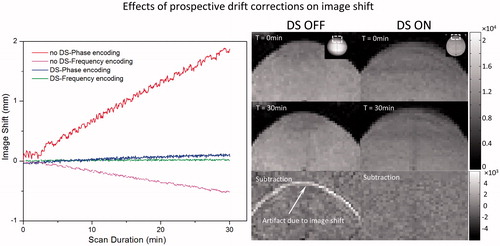
Figure 7 depicts the shift in image position that is caused by phase drift during a 30 min scan. A displacement of 1.8 mm (∼1 pixel) is apparent along the phase encoding direction after 30 min of scanning, and the rate of shift is linear (0.06 mm/min, R² = 0.995) over time. A much smaller shift of 0.5 mm along the frequency encoding direction was observed after 30 min. After enabling DS, the image shift was well corrected in both directions (Figure 7(A)). Figure 7(B) shows the corresponding magnitude images for the first and last dynamic scans, and a subtraction of the two images showing the non-zero residual at the edge of the phantom.

Figure 7. Correction of phase-induced image shift using F₀ dynamic stabilisation (DS). In the absence of DS, there is a gradual shift in image position along the phase encoding direction over time, corresponding to approximately 1 mm after 15 min of scanning (upper curve, red). A negative shift (<0.5 mm after 30-min scan) is observed along the frequency encoding direction (lower curve, pink). Both image shifts are corrected after applying DS (middle curves, blue and green). Right panel are corresponding magnitude maps showing the position shift over time with DS turned on/off.

Influence of slice-by-slice DC correction on phase drift

When performed alone, the slice-by-slice DC drift correction algorithm was able to address the magnitude and the changing rate of zero-order coefficients (Figure 6(A) and 6(B), blue). Moreover, when paired with DS enabled, the DC drift correction algorithm was able to remove the variability introduced by DS (Figure 6(B), green). By applying DS during the image acquisition and DC drift correction algorithm on the reconstructed data, the first-order coefficient along the AP direction was further reduced as well (Figure 6(C), green).

Influence of proposed drift correction strategies on accuracy of MR thermometry

Figure 8 indicates the results of the temperature validation experiments performed in a tissue-mimicking phantom as described in Figure 2. Four conditions were plotted in this figure: raw data (No Correction), DS only (DS), retrospective correction only (DC+3D) and the combined drift correction strategy (DS and DC+3D). Figure 8(A) and 8(B) show the results for probes 1 and 2, representing for heated and unheated region, respectively. Table 2 summarises the results from nine validation experiments performed under different conditions. From the figure it is clear that the best correspondence with the implanted fibre-optic sensor was achieved when both DS was enabled and the DC+3D drift correction algorithm was applied. In this case, the DC drift correction embedded in the retrospective correction algorithm was also able to reduce the noise introduced by DS.

Figure 8. Comparison is made between fibre-optic measurements and MR thermometry using various drift correction strategies: raw data (No Correction) dynamic stabilisation only (DS), DC+ 3D drift correction algorithm only (DC+ 3D), and combined strategy (DS and DC+ 3D). The drift correction algorithm validated here is the combination of DC drift correction and 3D first order drift correction. Panels A and B represent data acquired at probe 1 and probe 2 (shown in the insert), representing the heated and unheated region, respectively.

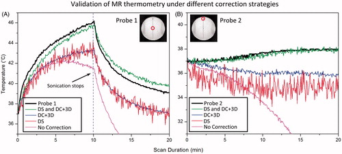
Table 2. Influence of F₀ dynamic stabilisation and different kinds of retrospective drift correction algorithm on the accuracy of temperature measurements with PRF-shift MR thermometry in a gellan gum phantom.

	Retrospective correction
Probe ID	Test ID	No correction	DC only	3D only	DC +3D
Probe 1 (Heated ROI)	Test 1	−21.84 ± 13.4	1.95 ± 1.08	1.80 ± 1.14	2.44 ± 1.49
No DS	Test 2	−16.28 ± 9.27	−2.42 ± 0.70	−1.84 ± 0.41	−1.54 ± 0.40
Δ Tin^^ C	Test 3	−7.22 ± 4.25	−2.06 ± 0.42	−2.20 ± 0.36	−1.89 ± 0.34
	Average (abs)	15.11 ± 8.97	2.14 ± 0.73	1.95 ± 0.64	1.96 ± 0.74
Probe 1 (Heated ROI)	Test 1	−2.43 ± 0.70	0.41 ± 0.39	0.53 ± 0.49	0.57 ± 0.40
With DS	Test 2	−1.65 ± 0.62	0.32 ± 0.49	0.38 ± 0.55	0.45 ± 0.52
Δ Tin^^ C	Test 3	−2.53 ± 0.96	0.63 ± 0.55	0.53 ± 0.54	0.60 ± 0.53
	Test 4	−1.99 ± 0.62	0.20 ± 0.50	0.28 ± 0.57	0.37 ± 0.53
	Test 5	−2.79 ± 1.05	1.30 ± 1.14	1.28 ± 1.17	1.40 ± 1.15
	Test 6	−2.34 ± 0.73	−0.10 ± 0.34	0.02 ± 0.48	0.04 ± 0.36
	Average (abs)	2.29 ± 0.78	0.49 ± 0.57	0.50 ± 0.63	0.57 ± 0.58
Probe 2 (Unheated ROI)	Test 1	−23.56 ± 13.78	−0.66 ± 0.64	−0.09 ± 0.91	0.53 ± 1.20
No DS	Test 2	−17.38 ± 10.69	−3.71 ± 2.04	−3.06 ± 1.20	−2.79 ± 1.05
Δ Tin^^ C	Test 3	−7.13 ± 5.19	−1.97 ± 1.27	−1.82 ± 0.79	−1.50 ± 0.78
	Average (abs)	16.02 ± 9.89	2.11 ± 1.32	1.66 ± 0.97	1.61 ± 1.01
Probe 2 (Unheated ROI)	Test 1	−2.89 ± 0.91	−0.04 ± 0.46	0.10 ± 0.49	0.14 ± 0.35
With DS	Test 2	−1.90 ± 0.64	0.33 ± 0.36	0.54 ± 0.45	0.61 ± 0.40
Δ Tin^^ C	Test 3	−4.71 ± 1.89	−1.55 ± 0.76	−0.83 ± 0.63	−0.75 ± 0.55
	Test 4	−2.58 ± 0.99	−0.39 ± 0.54	−0.44 ± 0.60	−0.35 ± 0.54
	Test 5	−2.12 ± 0.87	1.14 ± 0.46	0.64 ± 0.43	0.76 ± 0.35
	Test 6	−1.86 ± 0.64	0.62 ± 0.39	0.58 ± 0.43	0.60 ± 0.35
	Average (abs)	2.68 ± 0.99	0.68 ± 0.50	0.52 ± 0.51	0.54 ± 0.42

Table 3. MR temperature measurements acquired in 16 rabbits treated with MR-HIFU hyperthermia. MR temperature mapping used both prospective and retrospective corrections, with pre-heating and F₀ dynamic stabilisation, and combined drift correction algorithm. Temperature is well maintained at 41–45 °C in treatment cells for the intended duration (Time in Range). During therapy, mean temperature in treatment cells is 42.3° ± 0.7 °C, with T10 and T90 of 43.3° ± 0.8 °C and 41.4° ± 0.7 °C. The rectum temperature is not affected by treatment (37.1° ± 0.3 °C, with a temporal SD of 0.3° ± 0.2 °C).

			Heated ROI (°C)
Therapy duration (min)	No. of animals	Time in range (min)	T-mean (°C)	T10 (°C)	T90 (°C)	Rectum temperature (°C)
10	5	10.8	42.3 ± 0.4	43.3 ± 0.6	41.2 ± 0.4	36.8 ± 0.3
20	6	20.8	42.1 ± 0.8	42.9 ± 1.0	41.1 ± 0.7	37.3 ± 0.2
40	5	40.4	42.4 ± 0.4	43.3 ± 0.5	41.2 ± 0.5	37.3 ± 0.3
Average	NA	NA	42.2 ± 0.6	43.2 ± 0.7	41.2 ± 0.6	37.1 ± 0.3

In the heated (target) region, the result was unacceptable with raw data, with a mean error of 15.11° ± 8.97 °C observed across three experiments. Applying DC+3D drift correction alone reduced the error to 1.96 ± 0.74 °C, but did not address the issue of image displacement. With only DS enabled, the image displacement was corrected, but the temperature error (2.29 ± 0.78 °C) was still not acceptable for mild hyperthermia treatments. In this circumstance, applying slice-by-slice DC drift correction further reduced the error to 0.49 ± 0.57 °C, and also reduced the temporal fluctuation caused by enabling DS. Similar results were obtained in an unheated (reference) region. Additional processing with a 3D first-order correction algorithm did not make a significant difference (0.57 ± 0.58 °C) in the heated region but provided a noticeable improvement in the unheated region: 0.54 ± 0.42 °C compared to 0.68 ± 0.50 °C. Hence, with DS enabled, the DC+3D drift correction algorithm can generate MR thermometry measurements with sufficient accuracy to meet the requirements for mild hyperthermia treatments in both the target region and the reference area. It is important to note that for all of these validation tests, a 10-min pre-heating imaging acquisition was applied.

In vivo evaluation of MR thermometry during long-duration thermal therapy

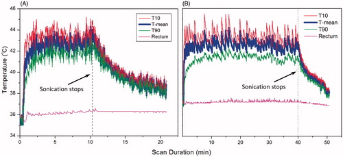
The coronal T2-weighted image in Figure 3(B) depicts a VX2 tumour implanted in a rabbit’s thigh, and indicates the position of a circular target ROI for hyperthermia. Figure 3(C) shows a temperature map acquired at 5 min after initiation of MR-HIFU hyperthermia. Temperature within the targeted area is well maintained at 41–43 °C, and the regions outside this area show no significant heating, indicating that the drift correction algorithm is functioning properly. Figure 9 shows the mean temperature, T10 and T90 within the target ROI during two mild hyperthermia treatments in rabbit thigh. The temperature is well maintained within the target range of 41–43 °C for both treatment durations: 10 min in Figure 9(A), and 40 min in Figure 9(B). MR temperature measurements summarised across 16 animals show a mean temperature of 42.2 ± 0.6 °C, T10 of 43.2 ± 0.7 °C and T90 of 41.2 ± 0.6 °C. The temperature in the rectum, measured with a fibre-optic probe, is included to indicate core body temperature. Across all animals, body temperature was 37.1 ± 0.3 °C, which confirms well-controlled localised heating in this animal model. For groups with treatment durations of 10, 20 and 40 min, the temperature within the heated region was maintained between 41–45 °C for 10.8, 20.8 and 40.4 min, respectively.

Figure 9. Temperature measured in a target region of rabbit muscle with MR thermometry during (A) 10 and (B) 40 min of hyperthermia. MR temperature maps were calculated from EPI acquisition, with pre-heating, F₀ dynamic stabilisation, and combined drift correction algorithm. The mean (T-mean, thick blue curve), T10, thin red upper curve (90th percentile) and T90, thin green lower curve (10th percentile) are shown in the graph. The temperature of the animal’s rectum during the treatment is plotted in the pink flat curve around 36-37 degree. The graphs indicate localised and well controlled heating in the target region with minimal heating of distal areas.

Discussion and conclusion

In this study, a phase drift correction pipeline including pre-scan imaging, F₀ dynamic stabilisation, and DC+3D retrospective drift correction was evaluated in conjunction with a clinical MR-HIFU system. By providing a temperature mapping accuracy of better than 1 °C for scan durations of 10 min, the proposed pipeline was proved to successfully deliver accurate MR thermometry for guidance of MR-HIFU hyperthermia.

Tissue ablation applications of MR-HIFU involve high temperature elevations (> 20 °C) for short periods of time (< 1 min), and PRF-shift MR thermometry meets the requirements for monitoring and controlling these treatments. For durations longer than 1 min, tissue swelling associated with thermal coagulation can introduce errors into the calculation of tissue temperature [64]. In the case of mild hyperthermia treatments involving MR-HIFU, mild heating in the range of 41–45 °C is generated in a larger volume of tissue (10–50 mm) over a much longer duration (up to 1 h). The desired therapeutic effects in tissue occur within a narrow temperature range, and are sensitive to short deviations. Therefore, the requirements for precise and accurate thermometry throughout treatment are quite strict. As an example, the application of targeted drug delivery using thermo-sensitive liposomes and mild hyperthermia has very strict requirements for temperature and time. Temperature elevations <40 °C are unlikely to achieve rapid release of drug at the heated site, while heating beyond 45 °C for extended periods could cause vascular damage, thereby limiting the ability of liposomes to penetrate the target volume for triggered release. Additionally, drug deposition is expected to increase with treatment duration up to 2 h of mild hyperthermia [65]. Therefore, strategies for accurate MR thermometry drift correction over tens of minutes are essential when considering the use of MR-HIFU for this clinical application.

The accuracy of the proposed multi-step drift-correction strategy was validated against an implanted fibre-optic probe in phantom experiments. After performing a 10-min pre-scan imaging to bring the scanner into a steady state, DS was enabled during acquisition to avoid the progressive displacement (approximately 2 mm after 30 min of scanning) in the reconstructed images. This displacement could introduce subtraction errors especially at tissue/organ boundaries. By adding DS, the main component of DC temperature drift was removed, but the temperature error (2.29 ± 0.78 °C) was still unacceptable for mild hyperthermia. Furthermore, DS introduced noise into the temperature maps because its centre frequency estimation has poor precision and applies one particular correction onto all slices in the stack. A slice-by-slice DC drift correction can remove this fluctuation by calculating the centre frequency offset from the complete image data of the previous dynamic instead of the phase navigators acquired before each dynamic. The last step was to perform the 3D first-order polynomial fit across all slices in the current dynamic. The final temperature error dropped to 0.57 ± 0.58 °C in the heated region and 0.54 ± 0.42 °C in an unheated region across six separate experiments, well within the requirements for hyperthermia. With these correction strategies utilised for hyperthermia treatments in a rabbit model, stable and precise measurements were obtained for long-duration heating between 10 and 40 min. Temperature was well-maintained within the target region without observing any signs of incomplete drift correction in surrounding tissues.

A few limitations of this study deserve mention. In the first experiment we aimed to characterise MRI hardware heating as a function of gradient duty cycle, and in turn the effect of scanner heating on phase drift. However, since temperature measurement of the gradients and passive shims during scanning was not possible, we measured the temperature of the inner plastic cover of the bore. The temporal response of gradient heating would be more delayed at this location, but as discussed above, may still serve as a useful surrogate of magnet temperature.

Another limitation is that fibre-optic probe validation tests were not performed in the rabbit experiment; this was due to the difficulty in placing the probe in the centre of the target region. Instead, validation tests used a phantom set-up that shared exactly the same imaging parameters as the rabbit experiment, and provided a more controlled environment to perform the validations. In addition, more configurations could be evaluated, and this set-up enabled us to determine the relative importance of prospective and retrospective corrections. The phantom used for validation experiments in this study was representative of the imaging conditions for MR-HIFU hyperthermia in rabbits. However, magnetic susceptibility distributions are likely to be more uniform in larger phantoms and humans, and the expected heating volume is likely to cover a smaller fraction of the tissue available for drift estimation. These factors would improve the precision of prospective F₀ dynamic stabilisation. They would also contribute to more accurate retrospective drift correction, with smaller contributions from first-order and higher-order spatial variations, and more voxels available for fitting. Furthermore, these experiments were all performed on a single MR scanner, while spatial and temporal drift characteristics can vary widely between MRI vendors, scanner models, and individual installations [42].

Finally, there are various methods available to perform accurate MR thermometry; however, the approach we describe represents a general method to correct the major effects of phase drift on MR thermometry accuracy over the long scanning durations associated with mild hyperthermia. Deviations from the baseline phase distribution can be estimated in reference phantoms of water [35,42] or oil [66,67] within the image. Extensions to higher order polynomial corrections or more extensive prospective corrections may further improve accuracy in cases of more severe background drift. Image shift artrfacts over long scanning durations can also be corrected using a retrospective approach by applying a rigid co-registration of incoming images to the baseline dynamic before subsequent polynomial fitting of phase drift [56,68]. In addition to phase drift, in vivo implementations of MR thermometry are very sensitive to tissue motion, which may be mitigated using accelerated acquisition with navigators [69] or multi-baseline and referenceless techniques [70,71].

Acknowledgements

Special thanks to Michelle Ladouceur-Wodzak, our veterinary technologist for her support in the preclinical experiments. Joris Nofiele and Cecil Futch assisted in the conduct of experiments described in the manuscript.

Disclosure statement

Financial support for this study was provided by the National Institutes of Health (1R01CA199037-01) and Cancer Prevention and Research Initiative of Texas (R1308). Philips Healthcare provided the clinical research platform and access to the drift correction algorithms through a sponsored research agreement with UT Southwestern Medical Center. Robert Staruch is an employee of Philips Research in the USA. Matti Tillander, Max O. Köhler and Mika Ylihautala are employees of Philips Healthcare in Finland. Charles Mougenot is an employee of Philips Healthcare in Canada. The other authors report no conflicts of interest. Philips Healthcare provides the clinical MR-HIFU system and the correction algorithms. The authors alone are responsible for the content and writing of the paper.

References

- Hynynen K, Darkazanli A, Unger E, Schenck JF. MRI-guided noninvasive ultrasound surgery. Med Phys 1993;20:107–15.
- Hynynen K, Damianou C, Darkazanli A, Unger E, Schenck JF. The feasibility of using MRI to monitor and guide noninvasive ultrasound surgery. Ultrasound Med Biol 1993;19:91–2.
- Cline HE, Schenck JF, Watkins RD, Hynynen K, Jolesz FA. Magnetic resonance-guided thermal surgery. Magn Reson Med 1993;30:98–106.
- Kim Y, Trillaud H, Rhim H, Lim HK, Mali W, Voogt M, et al. MR thermometry analysis of sonication accuracy and safety margin of volumetric MR imaging-guided high-intensity focused ultrasound ablation of symptomatic uterine fibroids. Radiology 2012;265:627–37.
- Stewart EA, Rabinovici J, Tempany CMC, Inbar Y, Regan L, Gastout B, et al. Clinical outcomes of focused ultrasound surgery for the treatment of uterine fibroids. Fertil Steril 2006;85:22–9.
- Tempany CMC, Stewart EA, McDannold N, Quade BJ, Jolesz FA, Hynynen K. MR imaging-guided focused ultrasound surgery of uterine leiomyomas: a feasibility study. Radiology 2003;226: 897–905.
- Huisman M, Lam MK, Bartels LW, Nijenhuis RJ, Moonen CT, Knuttel FM, et al. Feasibility of volumetric MRI-guided high intensity focused ultrasound (MR-HIFU) for painful bone metastases. J Ther Ultrasound 2014;2:16.
- Gianfelice D, Gupta C, Kucharczyk W, Bret P, Havill D, Clemons M. Palliative treatment of painful bone metastases with MR imaging-guided focused ultrasound 1. Radiology 2008;249:355–63.
- Hurwitz MD, Ghanouni P, Kanaev S V, Iozeffi D, Gianfelice D, Fennessy FM, et al. Magnetic resonance-guided focused ultrasound for patients with painful bone metastases: phase III trial results. J Natl Cancer Inst 2014;106:dju082.
- Wintermark M, Druzgal J, Huss DS, Khaled MA, Monteith S, Raghavan P, et al. Imaging findings in MR imaging-guided focused ultrasound treatment for patients with essential tremor. Am J Neuroradiol 2013;35:891–6.
- Dobrakowski PP, Machowska-Majchrzak AK, Labuz-Roszak B, Majchrzak KG, Kluczewska E, Pierzchała KB. MR-guided focused ultrasound: a new generation treatment of Parkinson’s disease, essential tremor and neuropathic pain. Interv Neuroradiol 20:275–82.
- Furusawa H, Namba K, Thomsen S, Akiyama F, Bendet A, Tanaka C, et al. Magnetic resonance-guided focused ultrasound surgery of breast cancer: reliability and effectiveness. J Am Coll Surg 2006;203:54–63.
- Hynynen K, Pomeroy O, Smith DN, Huber PE, McDannold NJ, Kettenbach J, et al. MR imaging-guided focused ultrasound surgery of fibroadenomas in the breast: a feasibility study. Radiology 2001;219:176–85.
- Zippel DB, Papa MZ. The use of MR imaging guided focused ultrasound in breast cancer patients; a preliminary phase one study and review. Breast Cancer 2005;12:32–8.
- Sommer G, Bouley D, Gill H, Daniel B, Pauly KB, Diederich C. Focal ablation of prostate cancer: four roles for magnetic resonance imaging guidance. Can J Urol 2013;20:6672–81.
- Chopra R, Colquhoun A, Burtnyk M, N’djin WA, Kobelevskiy I, Boyes A, et al. MR imaging-controlled transurethral ultrasound therapy for conformal treatment of prostate tissue: initial feasibility in humans. Radiology 2012;265:303–13.
- Chopra R, Baker N, Choy V, Boyes A, Tang K, Bradwell D, et al. MRI-compatible transurethral ultrasound system for the treatment of localized prostate cancer using rotational control. Med Phys 2008;35:1346–57.
- Napoli A, Anzidei M, De Nunzio C, Cartocci G, Panebianco V, De Dominicis C, et al. Real-time magnetic resonance-guided high-intensity focused ultrasound focal therapy for localised prostate cancer: preliminary experience. Eur Urol 2013;63:395–8.
- Staruch RM, Hynynen K, Chopra R. Hyperthermia-mediated doxorubicin release from thermosensitive liposomes using MR-HIFU: therapeutic effect in rabbit Vx2 tumours. Int J Hyperthermia 2015;31:118–33.
- Hijnen NM, Heijman E, Köhler MO, Ylihautala M, Ehnholm GJ, Simonetti AW, et al. Tumour hyperthermia and ablation in rats using a clinical MR-HIFU system equipped with a dedicated small animal set-up. Int J Hyperthermia 2012;28:141–55.
- Partanen A, Yarmolenko PS, Viitala A, Appanaboyina S, Haemmerich D, Ranjan A, et al. Mild hyperthermia with magnetic resonance-guided high-intensity focused ultrasound for applications in drug delivery. Int J Hyperth 2012;28:320–36.
- Salgaonkar VA, Prakash P, Rieke V, Ozhinsky E, Plata J, Kurhanewicz J, et al. Model-based feasibility assessment and evaluation of prostate hyperthermia with a commercial MR-guided endorectal HIFU ablation array. Med Phys 2014;41:033301.
- Tillander M, Hokland S, Koskela J, Dam H, Andersen NP, Pedersen M, et al. High intensity focused ultrasound induced in vivo large volume hyperthermia under 3D MRI temperature control. Med Phys 2016;43:1539.
- Dewhirst MW, Viglianti BL, Lora-Michiels M, Hanson M, Hoopes PJ. Basic principles of thermal dosimetry and thermal thresholds for tissue damage from hyperthermia. Int J Hyperthermia 2003;19:267–94.
- van der Zee J, González González D, van Rhoon GC, van Dijk JD, van Putten WL, Hart AA. Comparison of radiotherapy alone with radiotherapy plus hyperthermia in locally advanced pelvic tumours: a prospective, randomised, multicentre trial. Dutch Deep Hyperthermia Group. Lancet 2000;355(9210):1119–25.
- Jones EL, Oleson JR, Prosnitz LR, Samulski T V, Vujaskovic Z, Yu D, et al. Randomized trial of hyperthermia and radiation for superficial tumors. J Clin Oncol 2005;23:3079–85.
- Issels RD, Lindner LH, Verweij J, Wust P, Reichardt P, Schem B-C, et al. Neo-adjuvant chemotherapy alone or with regional hyperthermia for localised high-risk soft-tissue sarcoma: a randomised phase 3 multicentre study. Lancet Oncol 2010;11:561–70.
- Ranjan A, Jacobs GC, Woods DL, Negussie AH, Partanen A, Yarmolenko PS, et al. Image-guided drug delivery with magnetic resonance guided high intensity focused ultrasound and temperature sensitive liposomes in a rabbit Vx2 tumor model. J Control Release 2012;158:487–94.
- Staruch R, Chopra R, Hynynen K. Localised drug release using MRI-controlled focused ultrasound hyperthermia. Int J Hyperthermia 2011;27:156–71.
- Grüll H, Langereis S. Hyperthermia-triggered drug delivery from temperature-sensitive liposomes using MRI-guided high intensity focused ultrasound. J Control Release 2012;161:317–27.
- Needham D, Dewhirst MW. The development and testing of a new temperature-sensitive drug delivery system for the treatment of solid tumors. Adv Drug Deliv Rev 2001;53:285–305.
- Kong G, Dewhirst MW. Hyperthermia and liposomes. Int J Hyperthermia 15:345–70.
- Hijnen N, Langereis S, Grüll H. Magnetic resonance guided high-intensity focused ultrasound for image-guided temperature-induced drug delivery. Adv Drug Deliv Rev 2014;72:65–81.
- de Smet M, Hijnen NM, Langereis S, Elevelt A, Heijman E, Dubois L, et al. Magnetic resonance guided high-intensity focused ultrasound mediated hyperthermia improves the intratumoral distribution of temperature-sensitive liposomal doxorubicin. Invest Radiol 2013;48:395–405.
- De Poorter J, De Wagter C, De Deene Y, Thomsen C, Ståhlberg F, Achten E. Noninvasive MRI thermometry with the proton resonance frequency (PRF) method: in vivo results in human muscle. Magn Reson Med 1995;33:74–81.
- Ishihara Y, Calderon A, Watanabe H, Okamoto K, Suzuki Y, Kuroda K. A precise and fast temperature mapping using water proton chemical shift. Magn Reson Med 1995;34:814–23.
- Köhler MO, Mougenot C, Quesson B, Enholm J, Le Bail B, Laurent C, et al. Volumetric HIFU ablation under 3D guidance of rapid MRI thermometry. Med Phys 2009;36:3521–35.
- Ramsay E, Mougenot C, Köhler M, Bronskill M, Klotz L, Haider MA, et al. MR thermometry in the human prostate gland at 3.0T for transurethral ultrasound therapy. J Magn Reson Imaging 2013;38:1564–71.
- McDannold N, Clement GT, Black P, Jolesz F, Hynynen K. Transcranial magnetic resonance imaging-guided focused ultrasound surgery of brain tumors. Neurosurgery 2010;66:323–32.
- Rieke V, Instrella R, Rosenberg J, Grissom W, Werner B, Martin E, et al. Comparison of temperature processing methods for monitoring focused ultrasound ablation in the brain. J Magn Reson Imaging 2013;38:1462–71.
- Lange T, Zaitsev M, Buechert M. Correction of frequency drifts induced by gradient heating in 1H spectra using interleaved reference spectroscopy. J Magn Reson Imaging 2011;33:748–54.
- El-Sharkawy AM, Schar M, Bottomley PA, Atalar E. Monitoring and correcting spatio-temporal variations of the MR scanner’s static magnetic field. MAGMA 2006;19:223–36.
- Peters RD, Henkelman RM. Proton-resonance frequency shift MR thermometry is affected by changes in the electrical conductivity of tissue. Magn Reson Med 2000;43:62–71.
- Sprinkhuizen SM, Konings MK, van der Bom MJ, Viergever MA, Bakker CJG, Bartels LW. Temperature-induced tissue susceptibility changes lead to significant temperature errors in PRFS-based MR thermometry during thermal interventions. Magn Reson Med 2010;64:1360–72.
- Boss A, Graf H, Müller-Bierl B, Clasen S, Schmidt D, Pereira PL, et al. Magnetic susceptibility effects on the accuracy of MR temperature monitoring by the proton resonance frequency method. J Magn Reson Imaging 2005;22:813–20.
- Zhou X, He Q, Zhang A, Beckmann M, Ni C. Temperature measurement error reduction for MRI-guided HIFU treatment. Int J Hyperthermia 2010;26:347–58.
- Wyatt CR, Soher BJ, MacFall JR. Correction of breathing-induced errors in magnetic resonance thermometry of hyperthermia using multiecho field fitting techniques. Med Phys 2010;37:6300–9.
- Hey S, Maclair G, de Senneville BD, Lepetit-Coiffe M, Berber Y, Köhler MO, et al. Online correction of respiratory-induced field disturbances for continuous MR-thermometry in the breast. Magn Reson Med 2009;61:1494–9.
- Peters NHGM, Bartels LW, Sprinkhuizen SM, Vincken KL, Bakker CJG. Do respiration and cardiac motion induce magnetic field fluctuations in the breast and are there implications for MR thermometry? J Magn Reson Imaging 2009;29:731–5.
- El-Sharkawy AM, Schär M, Bottomley PA, Atalar E. Monitoring and correcting spatio-temporal variations of the MR scanner’s static magnetic field. Magn Reson Mater Physics Biol Med 2006;19:223–36.
- Peters RTD, Hinks RS, Henkelman RM. Ex vivo tissue-type independence in proton-resonance frequency shift MR thermometry. Magn Reson Med 1998;40:454–9.
- Shmatukha A V, Bakker CJG. Correction of proton resonance frequency shift temperature maps for magnetic field disturbances caused by breathing. Phys Med Biol 2006;51:4689–705.
- Barkauskas KJ, Lewin JS, Duerk JL. Variation correction algorithm: analysis of phase suppression and thermal profile fidelity for proton resonance frequency magnetic resonance thermometry at 0.2 T. J Magn Reson Imaging 2003;17:227–40.
- Rieke V, Vigen KK, Sommer G, Daniel BL, Pauly JM, Butts K. Referenceless PRF shift thermometry. Magn Reson Med 2004;51:1223–31.
- Svedin BT, Payne A, Parker DL. Respiration artifact correction in three-dimensional proton resonance frequency MR thermometry using phase navigators. Magn Reson Med 2015 Aug.
- Liu HL, Kochunov P, Lancaster JL, Fox PT, Gao JH. Comparison of navigator echo and centroid corrections of image displacement induced by static magnetic field drift on echo planar functional MRI. J Magn Reson Imaging 2001;13:308–12.
- Gellermann J, Wlodarczyk W, Hildebrandt B, Ganter H, Nicolau A, Rau B, et al. Noninvasive magnetic resonance thermography of recurrent rectal carcinoma in a 1.5 Tesla hybrid system. Cancer Res 2005;65:5872–80.
- Depoorter J, Dewagter C, Dedeene Y, Thomsen C, Stahlberg F, Achten E. The proton-resonance-frequency-shift method compared with molecular diffusion for quantitative measurement of two-dimensional time-dependent temperature distribution in a phantom. J Magn Reson Ser B 1994;103:234–41.
- Irarrazabal P, Meyer CH, Nishimura DG, Macovski A. Inhomogeneity correction using an estimated linear field map. Magn Reson Med 1996;35:278–82.
- Bing C, Ladouceur-Wodzak M, Wanner CR, Shelton JM, Richardson JA, Chopra R. Trans-cranial opening of the blood-brain barrier in targeted regions using a stereotaxic brain atlas and focused ultrasound energy. J Ther Ultrasound 2014;2:13.
- Morris H, Rivens I, Shaw A, Haar G Ter. Investigation of the viscous heating artefact arising from the use of thermocouples in a focused ultrasound field. Phys Med Biol 2008;53:4759–76.
- Partanen A, Yarmolenko PS, Viitala A, Appanaboyina S, Haemmerich D, Ranjan A, et al. Mild hyperthermia with magnetic resonance-guided high-intensity focused ultrasound for applications in drug delivery. Int J Hyperthermia 2012;28:320–36.
- Enholm JK, Köhler MO, Quesson B, Mougenot C, Moonen CTW, Sokka SD. Improved volumetric MR-HIFU ablation by robust binary feedback control. IEEE Trans Biomed Eng 2010;57:103–13.
- McDannold N, Hynynen K, Jolesz F. MRI monitoring of the thermal ablation of tissue: effects of long exposure times. J Magn Reson Imaging 2001;13:421–7.
- Gasselhuber A, Dreher MR, Partanen A, Yarmolenko PS, Woods D, Wood BJ, et al. Targeted drug delivery by high intensity focused ultrasound mediated hyperthermia combined with temperature-sensitive liposomes: computational modelling and preliminary in vivovalidation. Int J Hyperthermia 2012;28:337–48.
- Kuroda K, Oshio K, Chung AH, Hynynen K, Jolesz FA. Temperature mapping using the water proton chemical shift: a chemical shift selective phase mapping method. Magn Reson Med 1997;38:845–51.
- Wyatt C, Soher B, Maccarini P, Charles HC, Stauffer P, Macfall J. Hyperthermia MRI temperature measurement: evaluation of measurement stabilisation strategies for extremity and breast tumours. Int J Hyperthermia 2009;25:422–33.
- de Senneville BD, Mougenot C, Moonen CTW. Real-time adaptive methods for treatment of mobile organs by MRI-controlled high-intensity focused ultrasound. Magn Reson Med 2007;57:319–30.
- Pichardo S, Köhler M, Lee J, Hynnyen K. In vivo optimisation study for multi-baseline MR-based thermometry in the context of hyperthermia using MR-guided high intensity focused ultrasound for head and neck applications. Int J Hyperthermia 2014;30:579–92.
- de Senneville BD, Roujol S, Moonen C, Ries M. Motion correction in MR thermometry of abdominal organs: a comparison of the referenceless vs. the multibaseline approach. Magn Reson Med 2010;64:1373–81.
- Grissom WA, Rieke V, Holbrook AB, Medan Y, Lustig M, Santos J, et al. Hybrid referenceless and multibaseline subtraction MR thermometry for monitoring thermal therapies in moving organs. Med Phys 2010;37:5014–26.