
Abstract
Purpose: We introduce a method for calculation of the ultimate specific absorption rate (SAR) amplification factors (uSAF) in non-uniform body models. The uSAF is the greatest possible SAF achievable by any hyperthermia (HT) phased array for a given frequency, body model and target heating volume.
Methods: First, we generate a basis-set of solutions to Maxwell’s equations inside the body model. We place a large number of electric and magnetic dipoles around the body model and excite them with random amplitudes and phases. We then compute the electric fields created in the body model by these excitations using an ultra-fast volume integral solver called MARIE. We express the field pattern that maximises the SAF in the target tumour as a linear combination of these basis fields and optimise the combination weights so as to maximise SAF (concave problem). We compute the uSAFs in the Duke body models at 10 frequencies in the 20–900 MHz range and for twelve 3 cm-diameter tumours located at various depths in the head and neck.
Results: For both shallow and deep tumours, the frequency yielding the greatest uSAF was ∼900 MHz. Since this is the greatest frequency that we simulated, we hypothesise that the globally optimal frequency is actually greater.
Conclusions: The uSAFs computed in this work are very large (40–100 for shallow tumours and 4–17 for deep tumours), indicating that there is a large room for improvement of the current state-of-the-art head and neck HT devices.
Introduction
Hyperthermia (HT) is an adjuvant therapy most commonly used in conjunction with radiotherapy (RT) [Citation1]. Studies have shown that RT + HT improves complete response, local control and survival rates compared to RT alone for breast cancer [Citation2], head and neck cancer [Citation2,Citation3], melanoma [Citation2,Citation4], liver cancer [Citation5], uterine cervical cancer [Citation6–13] as well as bladder and rectal cancers [Citation9,Citation10]. Despite this rather large amount of evidence of the effectiveness of RT + HT, HT therapy is not clinically widespread. There are two major technical reasons for this. First, it is difficult to create a highly localised heating zone conformal to the target tumour. Second, even if this was possible, it is not straightforward to verify the thermal dose delivered. These challenges are especially pronounced for tumours deeper than 3 cm in the body. Thermal dose monitoring at these depths may ultimately require integrated HT and magnetic resonance imaging (MRI) thermometry [Citation14–17].
Electromagnetic (EM) radiofrequency (RF) and microwave (MW) phased arrays have been shown to produce somewhat focal heating regions. In phased arrays HT, the phase and amplitude of the transmit antennas are optimised to create a constructive interference pattern at the tumour location and destructive interferences everywhere else. When optimising HT phased array designs, there are four main design parameters to consider: The frequency of the treatment energy, the type of antennas (e.g. dipoles, monopoles, horns) and the number and spatial arrangement of the antennas. Seebass et al. [Citation18] used finite element modelling to simulate HT in five realistic patient models using dipole antennas arranged on a z-cylinder (z is the head–foot direction of the patient) with elliptic cross section. The target was the pelvis. The antennas modelled have 1, 2 and 3 rings in the z-direction and as many as 12 antennas per ring. Three treatment frequencies were modelled: 100, 150 and 200 MHz. The authors found that the 3-ring, 12 antennae-per-ring design performed best at all frequencies and that the best operating frequencies was 200 MHz. Paulides et al. [Citation19] simulated head-neck HT phased arrays with 1, 4, 6, 8 and 16 transmitting dipoles arranged in a single z-ring. Seven operating frequencies were modelled between 100 and 915 MHz. For all frequencies, array performance improved when increasing the number of dipole antennas. The best frequency for heating a 4 cm cube in the neck was 433 MHz. Interestingly, the optimal frequency was found to vary with the volume of the target: Higher (smaller) frequencies tended to do better for small (large) volumes. Kok et al. [Citation20] also showed in simulations that devices with multiple z-ring tend to do better than single-ring designs for a pelvic target. Besides these studies, other simulation studies have focussed on modelling existing devices, such as the BSD Sigma 60 applicator (Pirexar, Salt Lake City, UT) [Citation21] and the Sigma Eye applicator (Pirexar, Salt Lake City, UT) [Citation22–24].
Taken as a whole, these studies show that (i) the more antennae, the better the HT performance; (ii) antennae should be distributed in z in addition to around the circumference of the patient and (iii) higher frequencies are more efficient at heating deep tumours. However, the precise relationship between the four key parameters of HT phased arrays (frequency, type of antennae and number and position of the antennae) and their impact on HT performance is complex, non-linear and depends on the target application.
In this work, we introduce a new metric: The ultimate SAR amplification factor (uSAF). In HT, SAR amplification factors (SAF) are defined as the ratio of the average SAR inside the tumour and outside the tumour. By definition, the uSAF is the greatest possible SAF achievable by any HT phased array for a given frequency, body model and heating target. The uSAF is an upper-bound metric solely limited by the dynamics of Maxwell’s equations in the body. Analysis of this ultimate metric may allow HT coil designers to determine the room for improvement of their coil designs. Indeed, if an HT array performs well compared to the ultimate in term of SAF, the coil designer knows that further optimisation of the device will not yield significant improvement in this metric. Alternatively, if an HT array’s SAF is low compared the uSAF, further optimisation of the device is warranted. Moreover, analysis of the uSAF maps may yield insights in how to improve the design. Finally, analysis of the uSAF as a function of tumour location and frequency of the treatment energy can provide key insights in the potential of HT in a way that is agnostic to specific HT antennae technology considerations.
Below are the specific contributions of this work:
We introduce a method for the computation of the uSAF in realistic, non-uniform body models.
We compute the uSAF in 12 head and neck tumours placed in the Virtual Family “Duke” body model (IT’IS Foundation, Zurich Switzerland) [Citation25] with material EM properties obtained from the Gabriel database [Citation26]. Tumours are all 3 cm in diameter.
We compute the uSAF metric for 10 treatment frequencies ranging from 20 to 900 MHz.
We compute SAR, temperature and thermal dose distributions associated with the uSAF at each tumour location and frequency.
We provide the maps computed in this work as well as the code necessary to compute the uHT in anybody model and for any tumour location/size online (http://ptx.martinos.org/index.php/Main_Page).
Methods
The overall flowchart of our methodology is summarised in .
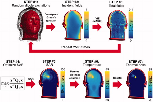
Figure 1. Flowchart of our methodology for computation of the ultimate SAF. STEP #1: The electric and magnetic dipoles in the dipole cloud are excited using random amplitudes and phases. STEP #2: The incident electric fields created by these excitations are computed using the analytical free-space Green’s function at the treatment frequency. STEP #3: Total electric fields are computed using the fast volume integral equation solver MARIE. Steps #1–#3 are repeated as many times as there are fields in the basis-set (2500 times in our case). STEP #4: The combination weights x applied to the basis fields are optimised so as to maximise the SAF in the target tumour volume. STEP #5: The SAR map associated with the SAF of STEP #4 is computed by applying the weights x to the basis fields. STEP #6: The temperature map is then computed by solving the Pennes bio-heat equation using the SAR map of STEP #5 as a source term. The input power of the SAR map is scaled so as to reach a maximum temperature of 45 degrees after 30 min of hyperthermia treatment. STEP #7: The thermal dose is computed by applying the CEM43 formula to the temperature histories computed in STEP #6.
Body model and tumour locations
We simulated the Duke body model (Virtual Family, IT’IS Foundation, Zurich Switzerland) [Citation25]. Duke contains more than 80 tissue types and is based on MRI scans of a 34 years old healthy male. We truncated the model below the neck in order to keep computational complexity to a minimum. We discretised Duke’s head and neck on a 3 mm isotropic resolution voxel grid, resulting in 193 542 non-zero voxels. We used the EM tissue properties tables published by Gabriel [Citation26] to generate permittivity and conductivity maps at treatment frequencies 21.3, 42.6, 63.9, 127.7, 200.1, 298.0, 400.2, 498.1, 596.1 and 894.1 MHz. These frequencies were chosen because they correspond to common frequencies used in MRI scanners and because they sample appropriately the 20–900 MHz frequency range. Operating HT at MRI carrier frequencies might be symbiotic since MRI scanners have RF power sources (>10 kW) at the needed frequency as well as the required shielding for operation outside the Industrial, Scientific and Medical (ISM) frequency bands.
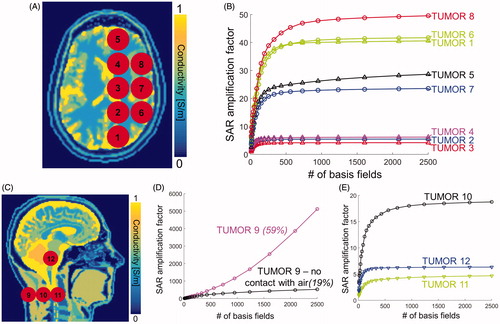
For each frequency, we computed the uSAF in twelve 3 cm-diameter spherical tumours in the head and neck (). This choice of the tumour diameter is on the small side of the tumour diameter distribution in clinical head and neck cancer patients [Citation27,Citation28], and, therefore, corresponds to a challenging treatment planning situation since it is harder to focus RF/MW energy in small volumes. Tumours #1–#12 are located at depth 3.1, 5.8, 6.5, 5.8, 3.5, 3.0, 3.5, 2.9, 1.0, 3.8, 5.4 and 6.4 cm in the body model (we define tumour depth as the distance between the tumour centre and the surface, or skin, of the body model). Our choice of tumour locations was not based on a statistical study of tumour locations as brain/neck tumours grow at every location in the head [Citation27,Citation28]. Instead, our locations were chosen to include both superficial and deep tumours in three general head regions: Supratentorial brain, infratentorial brain and neck. We did not explicitly model the 10–20% greater permittivity and conductivity of tumour tissues compared to healthy tissues [Citation29–31] since this would have required modification of the body model for the 12 tumour locations studied.
Figure 2. A: Conductivity map in the transverse view overlaid with the modelled tumour locations #1–#8. B: Convergence of SAR amplification factors (SAF) as a function of the number of basis fields in the basis-set for eight of the twelve tumour locations (F = 127.7 MHz). C: Conductivity map in the sagittal view overlaid with the last four tumour locations. D: Convergence of the SAF as a function of the number of basis fields for tumour #9 (F = 127.7 MHz). The purple curve corresponds to the original tumour #9 in direct contact with air. The black curve corresponds to a modified version of tumour #9 in which a 1-voxel thick layer of skin was added between the tumour and air. The two numbers above these curves indicate the percent change of SAF per additional 1000 basis field. E: Convergence of SAFs at F = 127.7 MHz as a function of the number of fields for tumour locations #10, #11 and #12.
Computation of electromagnetic basis-set in Duke
For the generation of the EM basis-set at a given frequency, we followed the strategy described by Guérin et al. [Citation32]. The approach is in three steps (). First, we place a large number of idealised electric and magnetic dipoles around the body model. The minimal distance between the dipoles and the body model is 3 cm in this work and the maximum distance is 3.5 cm. The difference between these two numbers (5 mm in this work) is the thickness of the dipole cloud. The minimum distance between the dipoles and the body model defines the antennal space in which the ultimate metric is valid. In other words, uSAF values computed in this work are the greatest SAF values achievable by any coil located at no less than 3 cm from the surface of the head and neck. This choice of 3 cm reflects the minimal buildable distance for a one-size-fits-all HT phased array. In fact, most HT applicators have their antennae located much further than 3 cm. For example, the head and neck applicator of Paulides et al. [Citation16] has a diameter of 30 cm and is, therefore, located at more than 5 cm from the head and 15 cm from the neck (the human head is ∼20 cm in the anterior–posterior direction and ∼17 cm in the left–right direction). Body applicators necessarily have a larger size. We chose the smallest realistic possible distance in order to explore the potential limits of SAF focussing. These parameters resulted in 43 977 dipole locations. We place six dipoles per dipole location (three X, Y and Z directions and two electric and magnetic dipoles per location), thus the total number of dipoles in our simulations is 263 862. We did not place dipoles below the neck as no coils can be placed there in reality.
We then excited the dipole cloud using random amplitudes and phases. As explained by Guérin et al. [Citation32], this is done in order to quickly generate a basis-set of EM fields that almost spans the space of solutions to Maxwell equations in the body model (the term “almost” is because that space in infinite, therefore, some truncation is required. However, our basis-set is convergent, i.e. the uSAF can be approximated to any desired accuracy by simply adding fields to the basis-set). Since storing the spatial field patterns of all the dipoles would require a large amount of memory, an SVD compression of all the dipole fields would be computationally laborious. Instead, we excite all the dipoles simultaneously using random amplitudes and phases, which allows quick construction of a basis-set of EM fields in the body model without having to compute all the dipole fields or hold them in memory [Citation32].
The second step is to compute the free space incident fields created by the random excitations of the dipole cloud. This can be done in a few seconds per excitation using analytical expressions of the dyadic Green’s function in free space at the simulated frequency. The last step, and the slowest as it can take 1–3 min per field, is to compute the scattered component of the field due to the presence of the body model. We compute it using a high-speed volume integral equation solver called MAgnetic Resonance Integral Equation (MARIE) which was developed specifically for biomedical applications and free to download at https://github.com/thanospol [Citation33].
This entire process is repeated K times, where K is the number of fields in the basis-set. In this work, we used K = 2500 since this number was sufficient to reach convergence in our previous calculation of the ultimate signal-to-noise ratio in MRI [Citation32]. We test that K = 2500 is a sufficient number of basis fields to achieve convergence in the estimation of the uSAF for all tumours and all frequencies in and Supplementary Figures 4 and 5.
Ultimate SAR amplification factor calculation
SAR amplification factor calculation
In this section, we describe how we maximised the SAF in the tumour, which is defined as SAF=SART/SARH, where SART is the average SAR in the tumour and SARH is the average SAR in healthy tissues located outside the tumour. To quickly compute the SAF, we use the following matrix representation of SAR: SAR=xHQx, where x is the vector of complex amplitudes (magnitude and phase) of the K basis fields and .H denotes the complex-conjugate operation. Q matrices are computed as:
(1) where P is the number of voxels in the mask (this is either the tumour mask or the body mask excluding the tumour), rp is the spatial location of voxel p, σ(rp) and ρ(rp) are the spatially varying conductivity and density and E(rp) is a K×3 matrix concatenating the electric fields of all K basis fields at location rp. We then optimise the SAF by solving:
(2) where QT and QH are the average SAR matrices in the tumour and healthy tissues (EquationEquation (1)
(1) ), respectively. This optimisation problem is concave and a solution is obtained by solving the generalised eigenvalue problem QTx=λQHx, which we compute using Matlab (Mathworks, Natick, MA).
Any electric field distribution in the body model, including the field pattern associated with the uSAF, can be represented with arbitrary accuracy by a linear combination of the fields in our convergent basis-set (the better the accuracy requested, the greater the number of basis fields needed). As pointed out below EquationEquation (2)(2) , the process of searching the weights of the basis field linear combination the maximum possible SAF has a unique, well-defined solution. Therefore, to check that our sequence of SAF converges to the ultimate SAF (uSAF) as we add basis fields, it is enough to plot this sequence as a function of the number of EM fields in the basis-set. Convergence is achieved if this sequence of SAF values plateaus, i.e. the SAF does not significantly increase as more fields are added to the basis-set. We use a convergence tolerance criterion of 5%.
Temperature and thermal dose calculation
To compute temperature, we solve the well-known Pennes bio-heat equation (PBHE):
(3) where T is the temperature and ρ, c and k are the local tissue density, specific heat capacity and thermal conductivity, respectively. In this equation, ρB, cB are the density and specific heat capacity of blood, TB is the blood temperature and ω is the local blood perfusion. We assume in this work a constant blood temperature of 37 °C. These parameters are spatially varying but we assume that they do not vary with temperature. We use standard values of the thermal conductivity, heat capacity and perfusion in the Duke model. For the tumours, we distinguish between the core, where the perfusion is assigned to 10% of the grey matter perfusion, and the penumbra, which is a ribbon of 3–6 mm thickness around the tumour core, and is, perfused twice as much as the grey matter. We solve the PBHE using a Crank–Nicholson finite time domain discretisation scheme that is unconditionally convergent [Citation34] with Dirichlet boundary conditions. The computational domain is shown in Supplementary Figure 1.
We compute temperature maps in two steps. First, we solve the PBHE with no SAR term for a duration of 1 h in order to establish the baseline temperature distribution. We do this because it is known that surface cooling creates a significant temperature differential between the centre of the brain (37 °C) and the skin surface (27 °C in our case as we assume that surface cooling occurs through contact with 20 °C ambient air, which is the temperature in most US hospitals) [Citation35]. Moreover, the CEM43 thermal dose formula depends on the absolute temperature distribution, not the relative temperature increase [Citation36], therefore, the absolute temperature needs to be simulated. We then solve the PBHE with a SAR term equal to the SAR distribution yielding the uSAF and an initial temperature distribution equal to the baseline temperature computed previously. The SAR distribution used as input to this simulation is scaled so as to obtain a maximum temperature of 45 °C at the end of the 30 min-long HT treatment. In order to find the input power yielding such a final peak temperature condition, we run multiple simulations and scale the input power by the ratio of the target temperature (45 °C) to the achieved maximum temperature until the desired peak temperature is achieved within 1%.
For each tumour location and frequency of the treatment energy, we compress the 30-min temperature history into a single thermal dose map. In this work, we use the cumulative equivalent minutes at 43 °C (CEM43) thermal dose [Citation36]. summarises all the computations performed in this study.
Table 1. Simulations and metrics of this study.
Results
Computation of basis-sets with K = 2500 fields for all 10 frequencies in Duke took a combined ∼22 d. The longest computation time was for 894.1 MHz (∼5 d), since the convergence of the MARIE solver slows at higher frequencies [Citation32,Citation33].
shows the convergence of the SAR amplification factors (SAFs) towards their ultimate value as a function of the number of fields in the basis-set for head tumours #1–#8. show the same thing for the remaining four tumours. The SAFs converged to their ultimate values (uSAF) for all tumours, except for #9, which, unlike all other tumours, is on the surface of the body model and in direct contact with air. In order to understand why the convergence of SAFs for tumour #9 is so different from the other tumour locations, we simulated a slightly modified version of this tumour that is not in direct contact with air by covering it with a 1-voxel layer of skin. shows that the SAF values for the modified tumour #9 are much lower than for the original tumour #9. In addition, the SAFs of the modified tumour #9 show improved convergence compared to the original tumour #9 (however, convergence is still not achieved as the SAF percent change per 1000 additional basis fields is equal to 19%, which is greater than our 5% convergence criterion). Supplementary shows that the uSAF calculation converged to better than 5% tolerance per 1000 basis fields for all tumours, except for tumour #9, and all frequencies. Supplementary shows that convergence is exponentially faster for deeper tumours than for shallow ones. Moreover, for deep tumours, convergence to the uSAF was faster for high treatment frequencies (for shallow tumours, there seems to be no significant dependence between the convergence rate and the frequency of the treatment energy).
Figure 3. USAFs as a function of the HT treatment frequency for tumours #1 through #12. The red numbers indicates, for each tumour location, the ratio of the highest to the lowest uSAF. In other words, this ratio indicates the expected improvement in SAF treatment efficacy by optimising the treatment frequency.
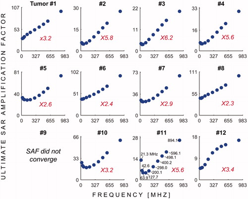
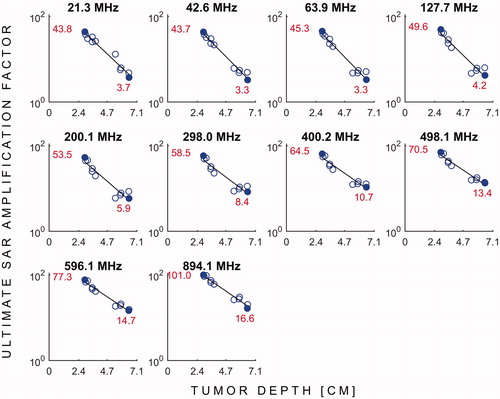
shows the uSAFs as a function of frequency for each tumours location. shows the uSAFs for each frequency plotted as a function of tumour depth. For frequencies above 127.7 MHz, the uSAF increased monotonically with frequency and reached a maximum at 894.1 MHz. For each tumour location, we calculated the ratio of the greatest to the lowest uSAF. This ratio was 2.3 for location #8 (depth =29 mm) and 6.2 for location #3 (depth =64 mm). Thus, for location #3, adjusting the frequency of the HT treatment in the range studied increased the uSAF by 520%. This ratio of maximum uSAF to minimum uSAF was consistently greater for deep tumour locations. Classifying locations 2, 3, 4, 10, 11 and 12 as deep, this ratio was equal to 5.0 in average for the deep tumours and 2.7 for the shallow tumours. Additionally, shows that the uSAF decreases approximately exponentially with tumour depth.
Figure 4. USAFs (log scale) as a function tumour depth for all the frequencies simulated. The red numbers and solid blue dots indicate the uSAFs for the shallowest and deepest tumour locations at each frequency.
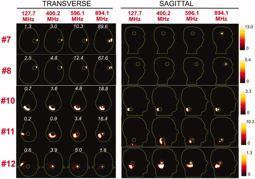
and show the SAR distributions associated with the uSAF for all tumours and all frequencies modelled. The input power is normalised so that the average SAR outside the tumour is equal to 3 W/kg. Visually, it is clear that the greater frequencies are better able to focus the EM energy selectively into the tumour volume while minimising it in the surrounding tissues (i.e. beamforming). Although this is easy for shallow tumours, the ultimate HT performance, as measured by the uSAF metric, is also very good for deep tumours, achieving double-digit SAFs for the deep tumours and close to triple-digit SAFs for the shallow ones. and show temperature maps obtained by solving the PBHE driven by the SAR source associated with the uSAF treatment and scaled so as to reach a maximum final temperature of 45 °C. The temperature amplification factor (TAF) is defined as the ratio of the average temperature inside the tumour to the average temperature outside of the tumour for the final temperature map. The TAFs are smaller than the SAFs shown in and , which is due to the fact that the heat equation acts as a smoothing kernel. Despite this, TAFs, like uSAFs, are quite large – the worst being for the midbrain tumour #12 (TAF =3.8) and the best, excluding tumour #9, being for the shallow grey matter tumour #6 (TAF =39.0). All TAFs are double-digits except for deep tumours #3, #11 and #12.
Figure 5. SAR maps (in W/kg) associated to the uSAF HT treatment for tumours #3–#6 at frequencies 127.7, 400.2, 596.1 and 894.1 MHz in both the transverse and sagittal views. Contours of the head and the tumour are shown in green. The white numbers indicate the uSAF for each tumour location and frequency simulated. USAFs are computed for the whole head and are, therefore, the same for the transverse and sagittal views.
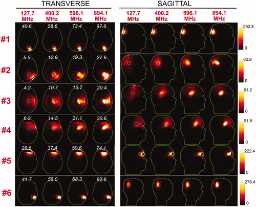
Figure 6. SAR maps (in W/kg) associated to the uSAF treatment for tumours #7–#12 at frequencies 127.7, 400.2, 596.1 and 894.1 MHz in both the transverse and sagittal views. Tumour #9 is not shown since the SAF did not converge to the ultimate value for this tumour location. Contours of the head and the tumour are shown in green. The white numbers indicate the uSAF for each tumour location and frequency simulated. USAFs are computed for the whole head and are, therefore, the same for the transverse and sagittal views.
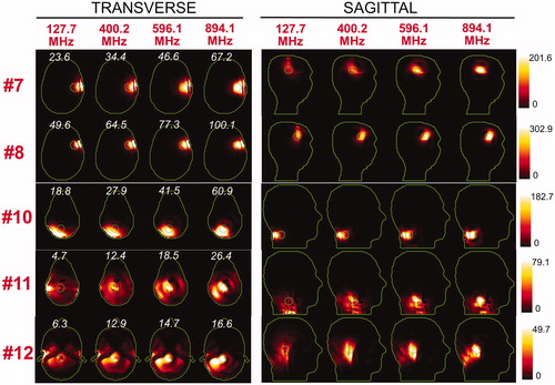
Figure 7. Temperature maps associated with the uSAF HT treatment for tumours #3–#6 and frequencies 127.7, 400.2, 596.1 and 894.1 MHz. The slices shown are transverse and sagittal views of the temperature volume though the centre of the tumours. Input SAR maps are scaled so as to achieve a maximum temperature of 45 degrees at the end of the 30-min HT treatment. Note that the maximum temperature is not necessarily achieved inside the tumour. Contours of the head and the target tumour ROI are shown in green. The white numbers indicate the temperature amplification ratio, which is the ratio of the average temperature increase inside and outside the tumour. Temperature amplification ratios are computed for the whole head and are, therefore, the same for the transverse and sagittal views.
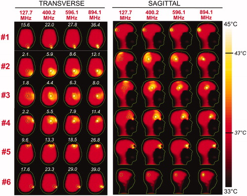
Figure 8. Temperature maps associated with the uSAF HT treatment for tumours #7–#12 and frequencies 127.7, 400.2, 596.1 and 894.1 MHz. Tumour #9 is not shown since the SAF did not converge to the ultimate value for this tumour location. The slices shown are transverse and sagittal views of the temperature volume though the centre of the tumours. Input SAR maps are scaled so as to achieve a maximum temperature of 45 degrees at the end of the 30-min HT treatment. Note that the maximum temperature is not necessarily achieved inside the tumour. Contours of the head and the target tumour ROI are shown in green. The white numbers indicate the temperature amplification ratio, which is defined as the ratio of the average temperature increase inside and outside the tumour. Temperature amplification ratios are computed for the whole head and are, therefore, the same for the transverse and sagittal views.
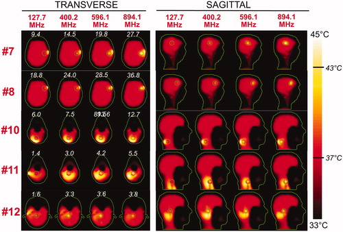
Although for all tumours the average temperature was always greater in the tumour than in surrounding tissue, Supplementary Figures 4 and 5 show that, for tumours #1, #6, #7, #8, #10, #11 and #12, the maximum temperature hotspot was in fact achieved in the healthy tissues. We point out that these tumours are immediately bordered by the skull, which is not highly perfused and is closer to the coil region; and, therefore, tends to be hotter than the target tumours.
and show maps of the CEM43 thermal dose associated with uSAF treatments simulated. These maps are much sparser than the temperature and SAR maps of . This is due to the fact that the thermal dose varies as ∼ RΔT, where ΔT is the temperature increase and R is a base factor equal to 0.25 for T ≤ 43 °C and 0.5 for T > 43 °C [Citation36]. This causes small local increases of the temperature to have an outsized impact in this metric [Citation36–38]. As a consequence, the thermal dose amplification factors are much larger than the uSAF when the EM energy is adequately focussed in the tumour. This is a double-edge sword; however, as they quickly decrease to small values when significant collateral heating is applied to healthy tissues.
Figure 9. Maps of the cumulative equivalent minute at 43 degrees (CEM43) thermal dose for tumours #1–#6, computed from the temperature histories of Figure 7. The white numbers indicate the thermal dose amplification ratio, which is the ratio of the average thermal dose inside and outside the tumour, for every tumour location and frequency. Thermal dose amplification ratios are computed for the whole head and are, therefore, the same for the transverse and sagittal views.
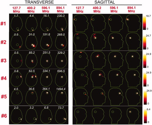
Figure 10. Maps of the cumulative equivalent minute at 43 degrees (CEM43) thermal dose for tumours #7–#12, computed from the temperature histories of Figure 7. Tumour #9 is not shown since the SAF did not converge to the ultimate value for this tumour location. The white numbers indicate the thermal dose amplification ratio, which is defined as the ratio of the average thermal dose inside and outside the tumour, for every tumour location and frequency. Thermal dose amplification ratios are computed for the whole head and are, therefore, the same for the transverse and sagittal views.
Discussion
Optimal frequency of the treatment energy for head and neck hyperthermia
We showed in this work that the best frequency of the treatment energy for head and neck HT is ∼900 MHz. Since 900 MHz was the maximum frequency simulated in this work, however, it is likely that the globally optimal frequency of the treatment energy is in fact greater than 900 MHz. This conclusion echoes previous studies that have found that MW frequencies are well suited to deep HT of small tumours [Citation18–20,Citation39]. Our uSAF results indicate that high frequencies are well suited to both deep and shallow head and neck HT: At 900 MHz, uSAFs ranged from 16.6 (deep midbrain tumour #12) to 100.1 (shallow brain tumour #8). This is considerably greater than the typical SAF values of existing HT devices and indicates a large room for improvement of currently used RF HT phase arrays.
Another finding is that the worst operating frequency was in the 20–128 MHz range for all the tumours simulated in this work, except tumour #9 which is an outlier in this study. This is noteworthy since this is precisely the range of operation of the two most commonly available HT devices: The Sigma 60 and the Sigma Eye. These two devices were designed for body HT and not the head, so this emphasises the need for development of head- and neck-specific HT devices operating at higher frequencies. Head and neck HT simulation studies have been performed previously that reached the same conclusion [Citation17,Citation19]. This study confirms this insight using the uSAF metric and suggests that even greater treatment frequencies than those previously studied should be used.
We found that the uSAFs decrease exponentially with tumour depth. This effect is similar to the skin depth effect, which causes EM waves to decay exponentially in conductive media. However, the ability of ultimate HT arrays to focus heat at deep locations partially compensate for the skin depth effect. For MW frequencies, we hypothesise that the competition between skin depth (which becomes smaller at increasing frequencies) and beamforming performance (which improves with increasing frequencies) leads to a globally optimal frequency. Beyond this frequency, absorption of EM waves is simply too pronounced to allow effective heating of deep tumours.
Most HT applicators operate at one of the allowed ISM frequencies to avoid interference with other RF devices: 27.12 MHz (worldwide), 40.68 MHz (worldwide), 433.92 MHz (Europe, Africa, Middle East, Russia and Mongolia), 915 MHz (Americas, Greenland and eastern Pacific islands) and 2.45 GHz (worldwide). Although these frequencies are convenient as they allow performing HT in an unshielded environment, operating outside the ISM bands can be done if the procedure is shielded. As a simulation study, we were not limited to ISM bands and we purposefully examined a larger range of frequencies. We also point out that the recent trend of combining MRI with HT is a strong rational for exploring frequencies outside of the ISM bands as MRI scanners are shielded and operate at 64, 128 and 300 MHz.
Convergence of the ultimate SAF metric
Supplementary Figure 2 shows that our uSAF calculation converged for all tumours and all frequencies except for tumour #9 (no frequency converged) as well as the two lowest frequencies of tumour #11. Tumour #9 is the only tumour location that was in direct contact with air in this study. Because of the sharp air-body EM property transition, electric fields created by the external dipole sources change very rapidly close to these locations. As we and others have shown in previous work on the use of EM basis-sets for computation of the ultimate signal-to-noise ratio in MRI [Citation32,Citation40–42], ultimate metrics converge more slowly at air-tissue interfaces than deep in body. Indeed, by simply adding a 1-voxel layer of tissue between tumour #9 and air (), SAF convergence was dramatically improved. Since the SAFs for tumour #9 did not converge, we do not claim to have an accurate estimation of the uSAF at this location. We do present convergence plots for this tumour in , however, as a cautionary tale of the difficulty to accurately compute the uSAF in superficial tumours. The convergence difficulties for tumour #11 were not as severe and we hypothesise, although it is not as simple to prove as for tumour #9, that this is due to the fact that this tumour contains vertebral bone. Since the EM properties of bone are very different from that of other tissues, the electric fields at this location also vary rapidly which in turn slows SAF convergence.
Hyperthermia treatment optimisation
SAF is a SAR-based metric that is widely used for HT arrays performance characterisation and treatment planning [Citation43]. However, as the temperature and thermal dose maps of clearly show, it is not equivalent to optimise SAR, temperature or the thermal dose. Ideally, the HT treatment plan should be optimised using the thermal dose as the final endpoint since this is the metric most directly related to the biological effects of HT [Citation1,Citation36]. Although direct thermal dose optimisation has been shown to be feasible [Citation44,Citation45], this is not widespread and is technically difficult. Moreover, existing methods for direct thermal dose optimisation are not convex and, therefore, do not guarantee convergence to the global optimum.
An alternative is to optimise the temperature distribution, which is well established for HT [Citation46–48]. However, direct temperature optimisation is feasible for HT arrays with at most a couple dozen antennae, but is difficult to apply to the uSAF computation. In this work, we used K = 2500 basis fields, which yields Hermitian SAR and temperature matrices of size 2500 × 2500 with each ∼3.1 million unique complex entries. Computation of temperature matrices following the strategy described by Das et al. [Citation46] would, therefore, require solving ∼3.1 million PBHEs. For the specific dimensions of the model used in this study, one PBHE solve took ∼2.5 min in Matlab so that sequential computation of temperature matrices would take ∼15 years! Even if computation time could be reduced to a reasonable value using parallel computing, storing the SAR and the temperature matrices in memory would require ∼10 TB of single precision memory as there is one 2500 × 2500 matrix per voxel location, which is beyond the capability of most computers. Therefore, computation of the ultimate temperature distribution will require the development of highly compressed and parallelised optimisation techniques and is not feasible yet.
Another limitation of the uSAF metric is that it only controls the average SAR outside the tumour. As others have pointed out [Citation44], this strategy typically creates large SAR hotspots outside the target heating zone. We have observed this phenomenon in the SAR and temperature maps of . To eliminate this problem, a possibility is to constrain SAR at all the body model locations outside the tumour mask. Compression could possibly be applied in order to reduce the number of SAR constraints [Citation49]. However, storage of all 193 542 SAR matrices in memory, which is required either for direct optimisation of SAR at all locations or for running the Virtual Observation Point compression algorithm [Citation49], requires ∼5 TB of RAM, which is impractical. A simpler solution could be to constrain SAR at a limited number of locations around the tumour, which may be sufficient to suppress the largest SAR hotspots in the healthy tissues. We will explore this strategy in future work.
Limitations of this work
Most HT devices include a water bath, which allows cooling the patient’ skin and improves EM coupling between the HT array and the body. We did not model a water bath in this work. A first reason for not doing so is that this would dramatically increase the size of the computational domain and therefore the complexity of the calculation. This would have forced us to increase the voxel size beyond 3 mm in order to fit the resulting volume integral equation (MARIE) problem in the memory of our Tesla K20 GPU card. This would have removed small but important features of the body model that are known to affect the position and intensity of SAR hotspots, such as details in the distribution of the cerebrospinal fluid (high-conductivity) and grey matter convolutions (medium conductivity) [Citation50]. Second, different devices use different water bath sizes, so that modelling a water bath in our ultimate SAF calculations would have rendered this metric not ultimate anymore. However, we recognise that the presence of the water bath may affect the distribution of electric fields in vivo and we propose to systematically study this effect in a subsequent publication.
We simulated the head and neck of the Duke body model without explicitly adding tumours to the voxel model. Instead, we studied the fundamental EM limit to creating focal temperature hotspots at 12 different spherical locations in the model. Tumours have a 10–20% greater permittivity [Citation29,Citation30] and conductivity [Citation29–31] than the surrounding healthy tissues, which is somewhat constant for many cancer types [Citation30]. Ideally, the greater permittivity and conductivity of tumours should be included in the body model. Doing so would require changing the body model for every tumour location, however, which would in turn require computing a new basis-set for every tumour location. In our case, this would dramatically increase computation from 22 to 264 d, which is not reasonable. We also point out that a 10–20% variation of the local tumour permittivity and conductivity is unlikely to dramatically affect our results and that such variation is probably smaller than the normal biological variability of EM tissue properties in vivo.
In this study, we simulated isotropic and temperature-independent tissue EM and thermal properties. It is known that some parameters, such as the perfusion and the electrical conductivity vary significantly with temperature [Citation38,Citation51,Citation52], therefore, it would be more accurate to model the temperature dependence of these parameters in our uSAF calculation. However, such a modification is not straightforward to incorporate in our framework. We also note that some tissues, such as brain white matter and muscles have anisotropic conductivity [Citation53,Citation54], but this is not commonly taken into account in EM modelling and is assumed to be have a minor impact on SAR.
Conclusions
In this work, we introduced a methodology for the computation of the ultimate SAR amplification factor (uSAF), which is the greatest SAF value achievable by any HT phased array. The SAF is defined as the ratio of SAR in the tumour and SAR outside the tumour. The first step in the method is to compute a convergent basis-set of EM fields in the body model of interest. In this work, we simulated the Duke body model, which is part of the Virtual Family. We then express the electric field distribution maximising the SAF in the target tumour as a linear combination of our basis fields with unknown combination weights. Finally, we solve for the weights maximising the SAF, which is a concave optimisation problem with a single optimum. We repeat this calculation with an increasing number of EM basis fields, and assess convergence by plotting the SAF as a function of the number of basis fields. We computed the uSAFs in Duke at 12 different tumour locations in the head and neck and 10 different frequencies in the 20–900 MHz range. Convergence of the uSAF calculation was achieved for all tumours that were not in direct contact with air (i.e. with at least one layer of skin voxels between the tumour and air). For all tumours not in contact with air, the most efficient frequency was 900 MHz. This suggests that MW HT offer a potential advantage for both deep and shallow tumours if practical considerations can be overcome.
Supplemental Files
Download Zip (8.6 MB)Disclosure statement
No potential conflict of interest was reported by the authors.
Additional information
Funding
Related Research Data
References
- Chicheł A, Skowronek J, Kubaszewska M, Kanikowski M. (2007). Hyperthermia–description of a method and a review of clinical applications. Rep Pract Oncol Radiother 12:267–75.
- Jones EL, Oleson JR, Prosnitz LR, et al. (2005). Randomized trial of hyperthermia and radiation for superficial tumors. J Clin Oncol 23:3079–85.
- Huilgol NG, Gupta S, Sridhar C. (2010). Hyperthermia with radiation in the treatment of locally advanced head and neck cancer: a report of randomized trial. J Cancer Res Ther 6:492.
- Overgaard J, Gonzalez Gonzalez D, Hulshof M, et al. (2009). Hyperthermia as an adjuvant to radiation therapy of recurrent or metastatic malignant melanoma. A multicentre randomized trial by the European Society for Hyperthermic Oncology. Int J Hyperthermia 25:323–34.
- Nagata Y, Hiraoka M, Nishimura Y, et al. (1997). Clinical results of radiofrequency hyperthermia for malignant liver tumors. Int J Radiat Oncol Biol Phys 38:359–65.
- Datta N, Bose A, Kapoor H, Gupta S. (1987). Thermoradiotherapy in the management of carcinoma cervix (stage IIIB): a controlled clinical study. Indian Med Gaz 121:68–71.
- Sharma S, Patel F, Sandhu A, et al. (1989). A prospective randomized study of local hyperthermia as a supplement and radiosensitizer in the treatment of carcinoma of the cervix with radiotherapy. Endocuriether/Hyperthermia Oncol 5:151–9.
- Hong-Wei C, Jun-Jie F, Wei L. (1997). A randomized trial of hyperthermo-radiochemotherapy for uterine cervix cancer. Chin J Clin Oncol 24:249–51.
- van der Zee J, González D, van Rhoon GC, et al. (2000). Comparison of radiotherapy alone with radiotherapy plus hyperthermia in locally advanced pelvic tumours: a prospective, randomised, multicentre trial. Lancet 355:1119–25.
- Zee J, Gonzalez DG. (2002). The Dutch deep hyperthermia trial: results in cervical cancer. Int J Hyperthermia 18:1–12.
- Vasanthan A, Mitsumori M, Park JH, et al. (2005). Regional hyperthermia combined with radiotherapy for uterine cervical cancers: a multi-institutional prospective randomized trial of the international atomic energy agency. Int J Radiat Oncol Biol Phys 61:145–53.
- Franckena M, Stalpers LJ, Koper PC, et al. (2008). Long-term improvement in treatment outcome after radiotherapy and hyperthermia in locoregionally advanced cervix cancer: an update of the Dutch Deep Hyperthermia Trial. Int J Radiat Oncol Biol Phys 70:1176–82.
- Harima Y, Nagata K, Harima K, et al. (2009). A randomized clinical trial of radiation therapy versus thermoradiotherapy in stage IIIB cervical carcinoma. Int J Hyperthermia 25:338–43.
- Gellermann J, Wlodarczyk W, Feussner A, et al. (2005). Methods and potentials of magnetic resonance imaging for monitoring radiofrequency hyperthermia in a hybrid system. Int J Hyperthermia 21:497–513.
- Stakhursky VL, Arabe O, Cheng KS, et al. (2009). Real-time MRI-guided hyperthermia treatment using a fast adaptive algorithm. Phys Med Biol 54:2131.
- Paulides M, Bakker J, Hofstetter L, et al. (2014). Laboratory prototype for experimental validation of MR-guided radiofrequency head and neck hyperthermia. Phys Med Biol 59:2139.
- Winter L, Oezerdem C, Hoffmann W, et al. (2015). Thermal magnetic resonance: physics considerations and electromagnetic field simulations up to 23.5 Tesla (1GHz). Radiat Oncol 10:201.
- Seebass M, Beck R, Gellermann J, et al. (2001). Electromagnetic phased arrays for regional hyperthermia: optimal frequency and antenna arrangement. Int J Hyperthermia 17:321–36.
- Paulides MM, Vossen SH, Zwamborn AP, van Rhoon GC. (2005). Theoretical investigation into the feasibility to deposit RF energy centrally in the head-and-neck region. Int J Radiat Oncol Biol Phys 63:634–42.
- Kok H, De Greef M, Borsboom P, et al. (2011). Improved power steering with double and triple ring waveguide systems: the impact of the operating frequency. Int J Hyperthermia 27:224–39.
- Canters R, Franckena M, Paulides M, Van Rhoon G. (2009). Patient positioning in deep hyperthermia: influences of inaccuracies, signal correction possibilities and optimization potential. Phys Med Biol 54:3923.
- Wust P, Fähling H, Wlodarczyk W, et al. (2001). Antenna arrays in the SIGMA-eye applicator: interactions and transforming networks. Med Phys 28:1793–805.
- Nadobny J, Fahling H, Hagmann MJ, et al. (2002). Experimental and numerical investigation of feed-point parameters in a 3-D hyperthermia applicator using different FDTD models of feed networks. IEEE Trans Biomed Eng 49:1348–59.
- Stauffer PR. (2005). Evolving technology for thermal therapy of cancer. Int J Hyperthermia 21:731–44.
- Christ A, Kainz W, Hahn EG, et al. (2010). The virtual family-development of surface-based anatomical models of two adults and two children for dosimetric simulations. Phys Med Biol 55:N23.
- Gabriel C. (1996). Compilation of the dielectric properties of body tissues at RF and microwave frequencies. DTIC Document.
- Wood JR, Green SB, Shapiro WR. (1988). The prognostic importance of tumor size in malignant gliomas: a computed tomographic scan study by the Brain Tumor Cooperative Group. J Clin Oncol 6:338–43.
- Jeremic B, Grujicic D, Antunovic V, et al. (1994). Influence of extent of surgery and tumor location on treatment outcome of patients with glioblastoma multiforme treated with combined modality approach. J Neurooncol 21:177–85.
- Stauffer P, Rossetto F, Prakash M, et al. (2003). Phantom and animal tissues for modelling the electrical properties of human liver. Int J Hyperthermia 19:89–101.
- Yoo DS. (2004). The dielectric properties of cancerous tissues in a nude mouse xenograft model. Bioelectromagnetics 25:492–7.
- O’Rourke AP, Lazebnik M, Bertram JM, et al. (2007). Dielectric properties of human normal, malignant and cirrhotic liver tissue: in vivo and ex vivo measurements from 0.5 to 20 GHz using a precision open-ended coaxial probe. Phys Med Biol 52:4707.
- Guérin B, Villena JF, Polimeridis AG, et al. (2016).The ultimate signal‐to‐noise ratio in realistic body models. Magn Reson Med. [Epub ahead of print]. DOI: 10.1002/mrm.26564.
- Polimeridis A, Villena J, Daniel L, White J. (2014). Stable FFT-JVIE solvers for fast analysis of highly inhomogeneous dielectric objects. J Comput Phys 269:280–96.
- Zhao JJ, Zhang J, Kang N, Yang F. (2005). A two level finite difference scheme for one dimensional Pennes’ bioheat equation. Appl Math Comput 171:320–31.
- Collins CM, Liu W, Wang J, et al. (2004). Temperature and SAR calculations for a human head within volume and surface coils at 64 and 300 MHz. J Magn Reson Imaging 19:650–6.
- Sapareto SA, Dewey WC. (1984). Thermal dose determination in cancer therapy. Int J Radiat Oncol Biol Phys 10:787–800.
- Dewhirst MW, Vigilanti BL, Lora-Michiels M, et al. (2003). Basic principles of thermal dosimetry and thermal thresholds for tissue damage from hyperthermia. Int J Hyperthermia 19:267–94.
- Song C, Park H, Lee C, Griffin R. (2005). Implications of increased tumor blood flow and oxygenation caused by mild temperature hyperthermia in tumor treatment. Int J Hyperthermia 21:761–7.
- Trefná HD, Vrba J, Persson M. (2010). Time-reversal focusing in microwave hyperthermia for deep-seated tumors. Phys Med Biol 55:2167.
- Ocali O, Atalar E. (1998). Ultimate intrinsic signal-to-noise ratio in MRI. Magn Reson Med 39:462–73.
- Wiesinger F, Boesiger P, Pruessmann KP. (2004). Electrodynamics and ultimate SNR in parallel MR imaging. Magn Reson Med 52:376–90.
- Lattanzi R, Sodickson DK. (2012). Ideal current patterns yielding optimal signal-to-noise ratio and specific absorption rate in magnetic resonance imaging: computational methods and physical insights. Magn Reson Med 68:286–304.
- Canters R, Wust P, Bakker J, Van Rhoon G. (2009). A literature survey on indicators for characterisation and optimisation of SAR distributions in deep hyperthermia, a plea for standardisation. Int J Hyperthermia 25:593–608.
- Köhler T, Maass P, Wust P, Seebass M. (2001). A fast algorithm to find optimal controls of multiantenna applicators in regional hyperthermia. Phys Med Biol 46:2503.
- De Greef M, Kok H, Correia D, et al. (2010). Optimization in hyperthermia treatment planning: the impact of tissue perfusion uncertainty. Med Phys 37:4540–50.
- Das SK, Clegg ST, Samulski TV. (1999). Computational techniques for fast hyperthermia temperature optimization. Med Phys 26:319.
- Kowalski ME, Jin JM. (2004). Model-based optimization of phased arrays for electromagnetic hyperthermia. Microw Theory Tech IEEE Trans 52:1964–77.
- Cheng KS, Stakhursky V, Craciunescu OI, et al. (2008). Fast temperature optimization of multi-source hyperthermia applicators with reduced-order modeling of ‘virtual sources’. Phys Med Biol 53:1619.
- Eichfelder G, Gebhardt M. (2011). Local specific absorption rate control for parallel transmission by virtual observation points. Magn Reson Med 66:1468–76.
- Kok H, Van Haaren P, Van de Kamer J, et al. (2005). High-resolution temperature-based optimization for hyperthermia treatment planning. Phys Med Biol 50:3127.
- Song CW. (1984). Effect of local hyperthermia on blood flow and microenvironment: a review. Cancer Res 44:4721s–30s.
- Vaupel P, Kallinowski F. (1987). Physiological effects of hyperthermia. Hyperthermia and the therapy of malignant tumors. Heidelberg: Springer, 71–109.
- Epstein B, Foster K. (1983). Anisotropy in the dielectric properties of skeletal muscle. Med Biol Eng Comput 21:51–5.
- Miklavčič D, Pavšelj N, Hart FX. (2006). Electric properties of tissues. Wiley encyclopedia of biomedical engineering. New York (NY): John Wiley & Sons.