Effect of applied voltage, duration and repetition frequency of RF pulses for pain relief on temperature spikes and electrical field: a computer modelling study

Abstract

Background: The thermal and electrical effects of pulsed radiofrequency (PRF) for pain relief can be controlled by modifying the characteristics of the RF pulses applied. Our goal was to evaluate the influence of such modifications on the thermal and electric performance in tissue.

Methods: A computational model was developed to compare the temperature and electric field time courses in tissue between a standard clinical protocol (45 V pulses, 20 ms duration, 2 Hz repetition frequency) and a new protocol (55 V pulses, 5 ms duration, 5 Hz repetition frequency) with a higher applied electric field but a smaller impact on temperature alterations in tissue. The effect of including a temperature controller was assessed. Complementarily, an agar-based experimental model was developed to validate the methodology employed in the computer modelling.

Results: The new protocol increased the electric field magnitude reached in the tissue by around +20%, without increasing the temperature. The temperature controller was found to be the fundamental factor in avoiding thermal damage to the tissue and reduced the total number of pulses delivered by around 67%. The experimental results matched moderately well with those obtained from a computer model built especially to mimic the experimental conditions.

Conclusions: For the same delivered energy, the new protocol significantly increases the magnitude of the applied electric field, which may be the reason why it is clinically more effective in achieving pain relief.

Keywords:

• Computational model
• electroporation
• pain relief
• pulsed radiofrequency
• temperature spike

Introduction

Radiofrequency (RF) energy is clinically used in pain management. In contrast to the wide area of the thermally coagulated zone manifested after continuous RF (CRF), pulsed RF (PRF) has demonstrated positive effects on pain treatment without provoking any permanent neurological disruptions [1–4]. While CRF causes pain relief by the effect of the tissue thermocoagulation creating irreversible injury to the target nerve, PRF involves lower temperatures (below 42–44 °C), which is considered to be the limit value at which no thermally induced necrosis is observed [5,6]. As a result, the PRF technique can be applied to the neural regions that have both sensory and motor fibres (e.g. peripheral nerves) without any risk of further motor deficits [7,8].

According to recent studies, there is no definitive explanation for the mechanisms involved in PRF. An exhaustive review of experimental observations regarding the potential PRF action mechanisms can be found in reference [9]. Different effects of exposure to PRF electrical fields have already been reported. Some studies have revealed evidence of morphological changes in the neuronal cells after PRF treatment that affect the inner structures of axons [1,10–12]. These structural changes consist of mitochondria swelling and disruption of the normal organisation of the microtubules and microfilaments that preferentially affect C-fibres and to a lesser extent Aδ fibres. In addition, transient ultrastructural changes such as endoneurial oedema and collagen deposition have also been found [13]. Besides structural changes, the effects on cellular activity and gene expression have also been observed [1,14,15] as well as an increase in the expression of inflammatory proteins [12]. All these effects could potentially inhibit the transmission of nerve signals through C-fibres, which would lead to pain relief [9].

It is widely accepted that the PRF action mechanism is most likely related to the induced electric field, rather than to thermal effects. Several explanations of how exposure to an electric field can lead to the observed structural effects have been proposed, including an alteration of the axonal membranes due to electroporation [16], an effect on the intracellular organelles due to the internal electric field [10] or a long-term depression of the synaptic transmission due to electrical stimulation [17]. However, to the best of our knowledge, no explanation has been postulated on how the electric field can trigger the observed changes in cellular activity and gene expression or the anti-inflammatory responses. A recent clinical study (employing a temperature control with the upper limit set at 42 °C) reinforces the hypothesis that the effects of PRF treatment are probably related to the electric field magnitude [18].

PRF has usually been based on a train of RF bursts (pulses) with a 10–20 ms duration and a 1–2 Hz repetition frequency [16,19]. The application of each burst provokes a temperature spike in the electrode tip that could have destructive thermal effects. It has been observed from both computer and experimental models that the longer pulse durations cause higher temperature spike magnitudes [16]. With this idea in mind, a new timing pattern consisting of pulses of 5 ms duration and 5 Hz repetition frequency is being clinically employed in an attempt to reduce temperature spike magnitude [20]. In addition, this new timing pattern is associated with the use of higher values of applied voltage (55 V instead of 45 V). Surprisingly, the impact of this new protocol (55 V–5 ms–5 Hz) on temperature spike magnitudes and electric field has not as yet been assessed. Although the clinical outcome of the new protocol should be assessed by clinical studies, the computer modelling technique can be a valuable tool for studying the thermal and electrical performance of RF-based clinical techniques.

With the foregoing considerations in mind, we planned a computer modelling study aimed at assessing the differences between the standard protocol (SP) (45 V pulses with 20 ms duration and 2 Hz repetition frequency [21,22]) and the new protocol (NP) (55 V pulses with 5 ms duration and 5 Hz repetition frequency [20]). An additional protocol (AP) consisting of 45 V pulses with 8 ms duration and 5 Hz repetition frequency was also considered, since it provides the same energy as the SP (20 ms × 2 Hz = 8 ms × 5 Hz = 40 ms/s) and employs the same repetition frequency as the NP protocol. In this way, the influence of the pulse duration on both the AP and NP protocols could be evaluated. The computer models also included a temperature controller, similar to the one implemented in RF generators used in clinical practice, to assess the impact of this controlling technique on the temperature spike magnitudes and electric field. A complementary in vitro study based on an agar phantom was also conducted to validate the methodology used in the computational models.

Materials and methods

Model geometry

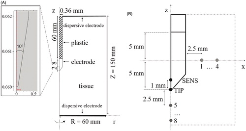
A PRF procedure was modelled with a 22-gauge needle electrode (0.64 mm in diameter) with a 10 mm long exposed tip. Figure 1(A) shows the two-dimensional model with three domains, consisting of muscle tissue, plastic cover (shaft) and electrode (exposed metallic part). The dispersive electrode (patch) was modelled as a zero voltage boundary condition on the outer boundaries (see Figure 1). The optimal dimensions of all the outer boundaries were established by means of a sensitivity analysis in which the maximum temperature reached at the electrode tip (T^MAX) was used as the control parameter. The dimensions were gradually increased until the difference of T^MAX between two subsequent simulations was less than 0.5%, after which the dimensions of the previous model were considered to be adequate.

Figure 1. (A) Geometry of the model including tissue, metallic electrode and plastic cover of the RF applicator. Dimensions in mm (out of scale). Note the detail of the electrode tip (scale in mm) consisting of a conical point with a 10° angle and rounded endpoint with an arbitrary 0.05 mm radius, which was assumed to avoid an infinite singularity in the model. (B) Specific locations chosen for evaluation of time course of electric field magnitude and temperature. Eight of these are separated from each other by 2.5 mm (P₁–P₄ in horizontal axis and P₅–P₈ in vertical axis). SENS corresponds to a point inside the conical tip of the electrode at a distance of 1 mm from its tip (TIP).

Material properties

The properties of the materials employed in the model are shown in Table 1. Tissue thermal conductivity (k) was assumed to be constant with temperature, while electrical conductivity (σ) was modelled as a temperature (T)-dependent function that grows exponentially +1.5%/°C at temperatures up to 99 °C [23]. Assuming that tissue temperature during PRF will stay below 99 °C, no desiccation due to water vaporisation was modelled. The electrical conductivity of muscle tissue (at 37 °C) was set to 0.28 S/m. This led to an impedance magnitude of approximately 350 Ω between the needle electrode and the dispersive electrode. This same value is typically found during PRF treatment under the same conditions as those used in this study and derives from the dielectric properties of the different tissues encountered along the path of the electric current. This value lies between those reported for muscle (0.45 S/m) and nerve (0.11 S/m) [24], and matches well with the physical situation in PRF, in which the electrode is inserted into muscle adjacent to a target nerve.

Table 1. Electric and thermal properties of materials and tissue [24,36,37].

Material	σ (S/m)	k (W/m·K)	ρ (kg/m^3)	c (J/kg·K)
Muscle	0.28^a	0.49	1090	3421
Plastic	10^−5	0.026	70	1045
Electrode	7.4 × 10^6	15	8 × 10^3	480

σ, electrical conductivity; k, thermal conductivity; ρ, density; c, heat capacity.

^a This value (at 37 °C) was considered in order to match the simulated initial impedance to the clinically observed values (∼350 Ω, see “Material properties” section).

Numerical model

The computational model was based on a coupled electric-thermal problem. A quasi-static approach was proposed for the solution. The governing equation for the electrical problem was (1) where V is the voltage, which is related with the electric field (E) by (2)

The thermal problem was solved using the Bioheat Equation: (3) where ρ is the density of tissue, c is the specific heat, k is the thermal conductivity, T is the temperature, t is the time, q is the heat source generated by RF power, Q_m is the metabolic heat generation (not considered in RF ablation) and Q_p is the heat loss from blood perfusion described as (4) where ω_b is the blood perfusion coefficient equal to 6.63 × 10^–4s^–1 (volume blood per unit mass tissue per unit time), ρ_b and c_b are the density and the specific heat blood of values 1000 kg/m³ and 4180 J/(kg·K), respectively and T_a is the temperature of the arterial blood (37 °C) [25]. The heat source q was taken from the electrical problem and evaluated as q = J · E, where J is the current density, which is obtained from J = σ E. No blood perfusion was assumed when tissue reached a 99% probability of thermal necrosis. The degree of thermal necrosis was estimated by a function based on the Arrhenius model: (5) where R is the universal gas constant, A is the frequency factor, 3 × 10⁴⁴ s⁻¹ and ΔE is the activation energy for the irreversible damage reaction, 2.90 × 10⁵ J/mol [26]. Thermal damage contours were estimated with the isolines Ω = 4.6 and Ω = 1, which correspond to a 99% and 63% probability of cell death, respectively. Regarding the electrical boundary conditions, no current was assumed on the symmetry axis or on the boundary parallel to it (see Figure 1). Voltage (45 or 55 V) was set at the electrode and applied as a pulse train, while 0 V was set at the boundaries of the tissue perpendicular to the symmetry axis. Thermal boundary conditions involved the temperature on external boundaries fixed at 37 °C. No heat flux was considered in the direction transverse to the symmetry axis. The initial temperature of the tissue was set to 37 °C.

Three protocols were considered. While a root-mean-square (RMS) voltage of 45 V is typically used in clinical practice with the SP, the NP usually involves higher magnitudes, values of 55 V [20] and even up to 60 V [27,28] have been proposed. Values of 45 V and of 55 V were simulated here. The value of 55 V combined with 5 ms–5 Hz is used, since it can deliver an energy value comparable with that of 45 V combined with 20 ms–2 Hz. This means that 20 ms–2 Hz with 45 V, 8 ms–5 Hz with 45 V and 5 ms–5 Hz with 55 V are equivalent protocols in terms of energy supplied to the tissue.

Analysis of thermal and electric performance

To analyse the thermal and electric performance, a set of points of interest were defined as shown in Figure 1(B). Thermal analysis included the temperature time course at an internal point of the sharp end of the electrode (SENS) and at the electrode point (TIP). For each pulse, the maximum (T^MAX) and minimum (T^MIN) temperatures reached in the tissue close to the electrode tip were analysed, along with the temperature spike magnitude (T^S) obtained as T^MAX−T^MIN. To be more precise, T^MAX was the temperature measured at the end of each pulse, while T^MIN was the lowest value reached just before starting the pulse. In the electric analysis, the RMS (root-mean-square) value of electric field magnitude (|E|) was assessed at point TIP and at eight locations in the tissue, equally distributed across radial (P₁–P₄) and axial directions (P₅–P₈) (see Figure 1(B)). These two directions were chosen as they are known to have different electric performances [16].

Temperature controller

The PRF procedure is habitually conducted with a temperature controller in order to avoid thermal lesions in the tissue due to excessive heating [19,29,30]. This control is achieved by means of a temperature sensor placed at the exposed sharpened tip of the electrode. To keep sensor temperature below the threshold of 42 °C, the applied voltage is modified accordingly, either by gradually reducing voltage or by transiently switching off the pulse application when tip temperature rises above the permitted maximum [1,7,10,14,21]. The SENS point shown in Figure 1(B) was defined specifically to mimic the location of the temperature sensor [16]. The temperature control was implemented in the model as an algorithm switching the input voltage between non-zero (on state) and zero value (off state). The state was determined in time by an implicitly defined event for which 42 °C and 41 °C measured at the SENS point were temperature set points for off and on states, respectively.

Meshing and model solver

A heterogeneous triangular mesh was used with 5312 elements and 25 578 degrees of freedom. A refinement in the area surrounding the electrode was applied. Mesh size was determined by a convergence test computed for the maximum tissue temperature (T^MAX) and was gradually increased until the differences in T^MAX between simulations were less than 0.5%. The criterion used for time step optimisation was the difference in temperatures, which was required to be less than 0.5 °C between two consecutive simulations. The model was solved by the Finite Element Method using COMSOL Multiphysics 5.1 software (COMSOL AB, Stockholm, Sweden).

Experimental validation

In order to validate the methodology used in the computational model, an experimental model based on an agar phantom (0.1% NaCl, dimensions 86.5 × 86.5 × 38 mm) was employed to obtain thermal and electrical measurements. Figure 2(A) shows an overview of the experimental setup. A disposable 18 G 10-mm RF electrode (St. Jude Medical, Saint Paul, MN) was inserted halfway into the agar phantom wall. A 0.1 mm-thick transparent polyethylene foil covering the wall of electrode insertion was used as an adiabatic window transparent to infra-red light. Two varnished copper wires (0.19 mm in diameter) were employed as probes to pick up the voltage value at 1 mm and 2 mm from the RF electrode surface. The wire tips were perpendicularly inserted 0.5 mm into the agar. Voltage differences with respect to the dispersive electrode of the RF generator were recorded with an Agilent DSO 1000 digital oscilloscope (Keysight Technologies, Santa Rosa, CA) at a sampling rate of 1 S/s. A PRF protocol of 20 ms × 2 Hz and 45 V pulses was applied during a 2-min period using an RF Neurotherm lesion generator (St. Jude Medical, Saint Paul, MN). Temperatures were recorded by FLIR Model E60 infra-red camera (FLIR Systems, Wilsonville, OR).

Figure 2. (A) Overview of the in vitro experimental setup based on an agar phantom. (B) Geometry of the computer model built to mimic the experimental setup (not to scale). The dispersive electrode was modelled on the wall parallel to the wall of electrode insertion.

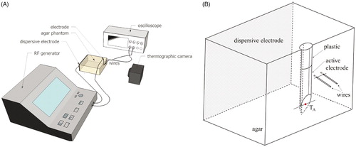
The validation was complemented with a computational model specifically designed to mimic the conditions of the experimental setup (see Figure 2(B)). Its main distinctive features were three-dimensional geometry, agar electrical conductivity of 0.31 S/m, no blood perfusion, ambient temperature of 21 °C and thermal insulation on the walls. The model also considered the presence of the voltage recording wires connected to the oscilloscope both thermally and electrically. These two wires not only acted as small thermal sinks but, since the input impedance of each channel was ∼20 kΩ at 500 kHz (input impedance 1 MΩǁ15 pF), stray RF current could flow from the electrode through the wires and the oscilloscope to the reference point. The model mimicked this phenomenon by adding an external circuit to the simulated domain consisting of two 20 kΩ resistors, one for each wire. The computer results (temperature distributions and progress of the voltage at 1 mm and 2 mm away from the RF electrode) were compared with those obtained from the experiments.

Results

Thermal performance

Figure 3 shows the last 2 s of the temperature time courses at points TIP and SENS for the SP (45 V–20 ms–2 Hz) for 6 min without TC. The courses were qualitatively similar at both points and were characterised by abrupt rises at the start of each RF pulse and decayed exponentially during off-periods between consecutive pulses. Table 2 shows the minimal and maximal temperatures, along with the temperature spike magnitude computed at both points for the three different timing patterns and two voltage values, as well as for the cases with and without TC. The main difference between the TIP and SENS points is that the T_SENS time course was a damped version of T_TIP. While T_TIP^S varied between 6.5 °C and 25.0 °C for all the cases considered, T_SENS^S only ranged from 0.4 to 2.7 °C. Interestingly, the temperatures registered at point SENS were generally very close to T_TIP^MIN values (differences of ∼1 °C).

Figure 3. Time course of the two last temperature spikes (in °C) at the electrode tip (T_TIP) and inside the electrode (T_SENS) after 6 min for the standard protocol (45 V–20 ms–2 Hz). The time course of T_SENS is presented in detail in the additional window. Note that temperature spike magnitude (assessed as: T^MAX – T^MIN) was much smaller at the SENS point.

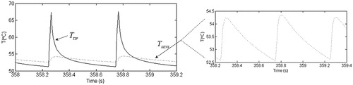
Table 2. Minimal (T ^MIN) and maximal (T ^MAX) temperatures, and temperature spikes (T ^S) assessed at the tip (TIP) and inside (SENS) the electrode after 6 min of PRF for different timing patterns (pulse duration × pulse repetition frequency) and applied voltages.

		Applied voltage
		45 V			55 V
Timing pattern	Location	T ^MIN (°C)	T ^MAX (°C)	T ^S (°C)	T ^MIN (°C)	T ^MAX (°C)	T ^S (°C)
20 ms × 2 Hz	SENS	52.6	54.3	1.7	61.2	63.9	2.7
	TIP	51.3	67.4	16.1	59.2	84.2	25.0
8 ms × 5 Hz	SENS	53.8	54.5	0.7	60.9	61.8	0.9
	TIP	52.7	61.6	8.9	60.4	73.9	13.5
5 ms × 5 Hz	SENS	47.4	47.8	0.4	52.9	53.5	0.6
	TIP	46.7	53.2	6.5	51.8	61.7	9.9
20 ms × 2 Hz (TC)	SENS	41.0	42.6	1.6
	TIP	40.6	56.8	16.2
5 ms × 5 Hz (TC)	SENS				41.0	42.1	1.1
	TIP				40.6	51.1	10.5

TC: cases with temperature controller (RF pulses were modulated in order to keep the temperature inside the electrode below 42 °C).

Figure 4(A–C) show the temperature distributions in the zone close to the electrode tip for the three protocols (SP, AP and NP) just after the last RF pulse in the absence of a temperature controller. As expected, the temperature at the electrode tip was maximal just at the end of each RF pulse. When the RF pulse ends, heat is evacuated towards the electrode body. Similar T_TIP^MAX values were found for AP and NP. In contrast, the temperatures obtained with the SP were ∼6 °C higher and a larger area surrounding the electrode tip reached high temperature values. The area of thermal lesion (assessed by contour Ω = 1) was similar for the three protocols and measured ∼0.5 mm thick in the direction transverse to the electrode axis.

Figure 4. Temperature distributions close to electrode tip just after applying the last RF pulse for different protocols without (A–C) and with (D,E) temperature controller. (A and D) Standard protocol (45 V–20 ms–2 Hz); (B) additional protocol (45 V–8 ms–5 Hz); (C and E) new protocol (55 V–5 ms–5 Hz). Black line is the damage contour Ω = 1 representing 63% of tissue damage. Note that the damage area is similar in (A–C), even though the maximum temperature reached in (A) is ∼6 °C higher, while no thermal lesion is observed in the cases with temperature controller (D–E).

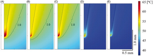
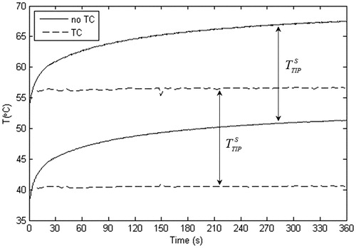
Likewise, Figure 4(D) and (E) show the temperature distributions in the zone close to the electrode tip for the SP and NP when the temperature controller was considered. As expected, the temperatures in the tissue showed the same spatial distribution as in the case with no temperature controller, but the absolute values were considerably lower. In fact, no thermal lesion was observed in any case. As shown in Table 2, the temperature controller kept T_SENS^MAX at ∼42 °C, which meant T_TIP^MIN in both cases was close to 41 °C. Since T_TIP^MAX and T_TIP^MIN were both reduced by ∼10 °C less than the cases with no TC, there was a negligible change of ∼0.6 °C in the temperature spike magnitude. As a consequence, although the TC considerably reduced both the maximum and minimum temperatures, it seemed to have no effect on the temperature spike magnitude (T_TIP^S was similar both with and without the TC). Note that both T_TIP^MAX and T_TIP^MIN reached a plateau after ∼21 s, which was approximately the time when T_MIN reached 42 °C and the controller came into action. The time evolution shown in Figure 5 was similar for the other protocols considered.

Figure 5. Comparison of time courses of maximal and minimal temperatures between the cases with and without temperature control (TC). Temperatures were assessed at the electrode tip and correspond with those of the standard protocol (45 V–20 ms–2 Hz).

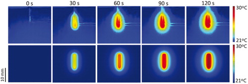
Regarding the thermal performance of the in vitro experimental study, the situation of the temperature evolution at point T_A (see Figure 2(B) for its location) was more or less comparable to that obtained from the corresponding computer model, with final temperatures of 26.73 ± 1.63 °C and 29.86 °C, in the experiments and simulations, respectively. The temperature measured at T_A was the maximum value registered by the camera. This value did not correspond to the highest temperature (which is usually expected to occur at the electrode tip point) since in this study the electrode tip was really embedded in the agar phantom. The temperature spikes in the experiments and simulations were similar (0.3 ± 0.1 °C vs. 0.2 °C). Figure 6 shows the temperature distributions of the experimental and computational models at 30 s intervals. The shape of the temperature distributions of the computer and experimental results was generally similar. While the thermal edge effect at the electrode tip was clearly visible in the experimental results (especially at 30 s), it was hardly noticeable in the computer results due to the plane view selected, which does not include the tip (see Figure 2(B)). Moreover, the high reflectivity associated with certain metal elements (e.g. electrode and wire zones) disturbed the temperature mapping and unfortunately could not be minimised.

Figure 6. Temperature distributions from the in vitro experiments (upper) and computer modelling (bottom) at different times. Note that the wires designed to pick up voltage in the experiments (except their non-insulated ends) are really outside the agar phantom and are consequently not part of the material surface.

Electrical performance

The values of the electric field magnitude |E| were quite stable during PRF application with no TC (|E| variation was negligible during each pulse). As the |E| value is directly dependent on the voltage applied, it was, therefore, higher for NP (55 V–5 ms–5 Hz) than for SP (45 V–20 ms–2 Hz). On this account, the |E| value for the AP protocol (45 V–8 ms–5 Hz) coincided with those obtained for the SP (45 V–20 ms–2 Hz).

When the TC was employed, the total number of applied pulses was considerably lower than the no TC case, with a reduction of 66.95% and 67.39% in SP and NP, respectively, while the |E| magnitudes remained practically unchanged. This finding suggests that although the tissue temperature could have a major effect on |E| through the σ(T) dependence, the spatial temperature gradients are too low to induce significant changes in the spatial distribution of σ between both models and hence there was no alteration in the magnitudes of the electric field.

Regarding the spatial distribution of the electric field, the highest |E| value for the last pulse was reached at the electrode tip and dropped rapidly with distance from the electrode surface, as was also observed with the temperature distribution. Table 3 shows the maximum values of |E| at various locations. Neither pulse duration nor repetition frequency had an impact on the |E| value of the last pulse.

Table 3. Electric field magnitudes (V/m) measured at specific locations (see Figure 1(B)) and at the end of the last RF pulse in the case of different timing patterns (pulse duration – pulses repetition frequency) and applied voltages (without temperature controller).

Applied voltage	45 V			55 V
Timing pattern	20 ms–2 Hz	8 ms–5 Hz	5 ms–5 Hz	20 ms–2 Hz	8 ms–5 Hz	5 ms–5 Hz
1	4106	4210	4165	5047	5015	5047
2	1892	1887	1837	2348	2390	2318
3	1080	1063	1022	1366	1395	1292
4	656	663	633	861	855	805
5	2329	2305	2237	2946	2958	2807
6	1018	1022	979	1325	1323	1242
7	612	605	576	789	801	734
8	413	406	385	532	542	492

The |E| value decayed as we moved away from the electrode surface, and this drop was stronger in the direction defined by the electrode axis (as shown in Figure 7(B)). For instance, for SP with 45 V, it decayed from 26.4 kV/m (computed at 0.1 mm from the electrode surface) to 4.1 kV/m at P₁, and from 60.9 kV/m (computed at 0.1 mm from the electrode surface) to 2.3 kV/m at P₅. For distances from the electrode surface (r) of up to 10 mm, the electric field decreased proportionally to 1/r in the direction transverse to the electrode axis and to 1/r² in the direction of the electrode axis.

Figure 7. Electrical potential distribution (V) during the last pulse of the 20 ms pulse duration protocol from the computational model based on the in vitro study using an agar phantom (A) and from the modelling study in tissue (45 V–20 ms–2 Hz) (B). Black contour lines represent electric field magnitude (V/m). Black dots are the points of voltage and field measurement from each model.

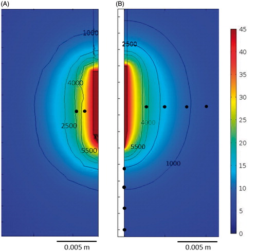
In the electrical performance in the in vitro experimental study, the voltage values measured at 1 and 2 mm distances at the beginning of the PRF application were very similar to those obtained from the computer model: 29.9 ± 3.2 V vs. 29.5 V and 24.3 ± 2.4 V vs. 24.3 V, respectively. There was also good agreement between the values at the end of the application: 30.9 ± 3.0 V vs. 30.5 V and 25.4 ± 2.0 V vs. 25.4 V. Figure 7(B) shows the voltage and electric field distributions from the computer model built to validate the experimental results, which are seen to be very similar to those obtained from the model that reproduced the clinical situation (Figure 7(A)).

Discussion

The aim of this study was to compare the performance of two different PRF protocols in terms of the temperature generated and, in particular, the electric field. First of all, we conducted an experimental PRF study on agar phantom in order to guarantee the accuracy of the computer model predictions and validate the modelling methodology. Even though the final temperature value was lower in the experiment than in the simulations, we found both results in reasonable agreement. One of the possible reasons for the measurement interference could have been the effect of the higher than expected heat losses, in addition to the fact that the metal electrode had much lower emissivity than the agar phantom for which the camera had been calibrated.

The thermal impact of PRF on tissue is defined by temperature spike phenomena within a range of independently modified maximum and minimum values that depend on the pulse protocol. As previously demonstrated by Cosman and Cosman [16], shorter pulses entail lower values of the temperature spike magnitude, while higher applied voltage and higher repetition frequency imply the opposite. In practical terms, the results confirmed that the new protocol (55 V–5 ms–5 Hz) has a similar thermal effect to that obtained with the standard protocol (45 V–20 ms–2 Hz) but with a considerably higher electric field magnitude due to the fact that both protocols provided equivalent total energy during the procedure.

When the temperature controller was included, the total applied pulses were considerably reduced (66.95% and 67.39%). This avoided thermal damage to the tissue (Figure 4(D,E)) even though the maximum temperatures at the electrode tip were close to 50 °C, neither did it have much effect on the electric field magnitude.

In order to optimise PRF protocols, it is necessary to maximise what can be defined as the “electrical dose” while minimising the thermal effects to avoid thermal injury, although it is no easy task to define this “electrical dose”. Experimental studies indicate that it cannot be defined as proportional to the delivered electrical energy, because protocols that apply similar heating yield different treatment outcomes [18]. Neither can it be defined as proportional to the product of the electric field magnitude and the active time (pulse duration × frequency) because that would imply that, for protocols of equivalent energy but different fields, the protocol with the highest “electrical dose” would have the lowest electric field, and experimental results show that this is not the case. As it appears that PRF efficacy strongly depends on the electric field magnitude, the “electrical dose” should, therefore, reflect this strong dependence on it. By increasing the applied voltage, the target tissue is exposed to a higher electric field, but this does not necessarily lead to an increase in the delivered energy – or in the thermal effects – if the pulses are shortened and the repetition frequency is reduced.

Since including the temperature controller reduced the total amount of applied pulses by 66.95% and 67.39% for SP and NP, respectively, we could estimate a “cumulative time” of equivalent continuous electric field application as the sum of the duration of all the pulses actually delivered, which would provide a “cumulative time” of 4.75 s and 2.93 s for SP and NP, respectively. This difference between the protocols should be taken into account in any future studies that might prove that the “electrical dose” is somehow related to this “cumulative time”.

Raising the voltage from 45 to 55 V caused a proportional rise in the electric field, which at a distance of 2.5 mm increased to over 500 V/m (along the radial axis) and 900 V/m (along the axial axis). As expected, the increase in electric field magnitude was approximately proportional to the increase in the applied voltage (≈+20%). It can therefore be inferred that this increase in |E| would have a significant impact on the outcome of the PRF treatment.

Another interesting finding was that the electric field magnitude shows a smaller decrease with distance in the direction transverse to the electrode axis, as compared to the direction parallel to it, which suggests that the “electrical dose” is also affected by the relative positioning of the electrode with respect to the target nerve. In the regions close to the electrode tip, the electric field magnitude may be large enough to cause cell electroporation. Due to their geometry, when nerve fibres are exposed to an electric field with a direction approximately parallel to their orientation, the induced transmembrane voltage is significantly larger than that experienced by other types of cells [31]. Therefore, the electric field necessary for electroporation to occur in nerve fibres is lower than in other cells. Although monopolar pulses are the most effective in terms of cell electroporation, pulsed AC fields are also known to cause it [32], and bursts of biphasic pulses in the same frequency range as those used in PRF have been shown to ablate tissues by means of irreversible electroporation [33].

Due to the lack of experimental studies in this area, it is not possible to indicate the electric field threshold necessary for the electroporation of nerve fibres to occur when using the typical PRF waveforms, although experiments performed with bursts of bipolar pulses can serve as a reference. On one hand, the electric field required to cause electroporation through these pulses is about 2.5 times larger than that of conventional monopolar pulses of the same duration [34]. On the other hand, in a study by Abramov et al. [35], electric pulses of 7.5 kV/m caused obvious signs of electroporation and, as a consequence, nerve conduction block, as well as disintegration of the myelin sheath and swelling of the nerve tissue in the rat sciatic nerve. We can, therefore, hypothesise that severe electroporation will occur in regions exposed to electric fields in the order of 18 kV/m and above, which, in our study, were only found very close to the electrode tip (distance <0.5 mm). Nevertheless, it should be noted that this value could have been lower due to the exposure time in PRF treatments being longer than conventional electroporation protocols. Neither can we rule out the occurrence of mild electroporation – which does not damage neurons – for much lower fields.

Limitations of the study

This study has some limitations that should be pointed out. First, the computer model represented a general approach to PRF used in pain treatment, but no specific location (target) for the PRF treatment was considered, i.e. the tissue was considered to be homogeneous. This simplification could introduce inaccuracies in the simulated model since non-homogeneous tissue presents a distorted electric field distribution. Also, instead of modelling different compartments, one material was used in the study whose electrical conductivity value was the result of the conductivities of the adjacent tissues. Second, only one specific RF applicator was modelled, regardless of the other sizes habitually employed in PRF clinical practice (diameters ranging from 18 to 22 gauges and lengths from 5 to 10 mm). In spite of these two limitations, we consider that the conclusions are still valid since this was a comparative study and the protocols considered were evaluated under identical conditions.

Conclusions

The recently proposed PRF protocol based on a higher voltage (55 V instead of 45 V), shorter pulses (5 ms instead of 20 ms) and a higher pulse frequency repetition (5 Hz instead of 2 Hz) can increase the electric field magnitude reached in the tissue without raising the temperature as the total time of exposure to RF is considerably reduced. However, what really avoids thermal damage is the use of a temperature controller, which keeps the electric field magnitude at the same level as when this system is absent and reduces the total delivered pulses by around 67%.

Disclosure statement

No potential conflict of interest was reported by the authors.

Additional information

Funding

This work was supported by the Spanish “Plan Estatal de Investigación, Desarrollo e Innovación Orientada a los Retos de la Sociedad” under Grant TEC2014-52383-C3-R (TEC2014-52383-C3-1-R and TEC2014-52383-C3-2-R). Elżbieta Ewertowska has a Predoctoral Grant (BES-2015–073285) from the Ministry of Economy, Industry and Competitiveness (Government of Spain).

References

- Protasoni M, Reguzzoni M, Sangiorgi S, et al. (2009). Pulsed radiofrequency effects on the lumbar ganglion of the rat dorsal root: a morphological light and transmission electron microscopy study at acute stage. Eur Spine J 18:473–8.
- Vas L, Pai R, Khandagale N, Pattnaik M. (2014). Pulsed radiofrequency of the composite nerve supply to the knee joint as a new technique for relieving osteoarthritic pain: a preliminary report. Pain Physician 17:493–506.
- Vallejo R, Benyamin RM, Kramer J, et al. (2006). Pulsed radiofrequency denervation for the treatment of sacroiliac joint syndrome. Pain Med 7:429–34.
- Cohen SP, Van Zundert J. (2010). Pulsed radiofrequency: rebel without cause. Reg Anesth Pain Med 35:8–10.
- Brodkey JS, Miyazaki Y, Ervin FR, Mark VH. (1964). Reversible heat lesions with radiofrequency current. A method of stereotactic localization. J Neurosurg 21:49–53.
- Viglianti BL, Dewhirst MW. (2011). Thresholds for thermal damage to normal tissues: an update. Int J Hyperthermia 27:320–43.
- Vatansever D, Tekin I, Tuglu I, et al. (2008). A comparison of the neuroablative effects of conventional and pulsed radiofrequency techniques. Clin J Pain 24:717–24.
- Heavner JE, Boswell MV, Racz GB. (2006). A comparison of pulsed radiofrequency and continuous radiofrequency on thermocoagulation of egg white in vitro. Pain Physician 9:135–7.
- Hata J, Perret-Karimi D, DeSilva C, et al. (2011). Pulsed radiofrequency current in the treatment of pain. Crit Rev Phys Rehabil Med 23:213–40.
- Erdine S, Bilir A, Cosman ER, Cosman ER. (2009). Ultrastructural changes in axons following exposure to pulsed radiofrequency fields. Pain Pract 9:407–17.
- Choi S, Choi HJ, Cheong Y, et al. (2013). Internal-specific morphological analysis of sciatic nerve fibers in a radiofrequency-induced animal neuropathic pain model. PLoS One 8:e73913.
- Choi S, Choi HJ, Cheong Y, et al. (2014). Inflammatory responses and morphological changes of radiofrequency-induced rat sciatic nerve fibres. Eur J Pain (United Kingdom) 18:192–203.
- Podhajsky RJ, Sekiguchi Y, Kikuchi S, Myers RR. (2005). The histologic effects of pulsed and continuous radiofrequency lesions at 42 °C to rat dorsal root ganglion and sciatic nerve. Spine (Phila Pa 1976) 30:1008–13.
- Lee J, Byun J, Choi I. (2015). The effect of pulsed radiofrequency applied to the peripheral nerve in chronic constriction injury rat model. Ann Rehabil Med 39:667–75.
- Van Zundert J, de Louw AJ, Joosten EJ, et al. (2005). Pulsed and continuous radiofrequency current adjacent to the cervical dorsal root ganglion of the rat induces late cellular activity in the dorsal horn. Anesthesiology 102:125–31.
- Cosman ER, Cosman ER. (2005). Electric and thermal field effects in tissue around radiofrequency electrodes. Pain Med 6:405–24.
- Sandkühler J, Chen JG, Cheng G, Randić M. (1997). Low-frequency stimulation of afferent Adelta-fibers induces long-term depression at primary afferent synapses with substantia gelatinosa neurons in the rat. J Neurosci 17:6483–91.
- Fang L, Tao W, Jingjing L, Nan J. (2015). Comparison of high-voltage-with standard-voltage pulsed radiofrequency of Gasserian Ganglion in the treatment of idiopathic Trigeminal Neuralgia. Pain Pract 15:595–603.
- Rohof OJ. (2002). Radiofrequency treatment of peripheral nerves. Pain Pract 2:257–60.
- Rohof OJ. (2014). Caudal epidural of pulsed radiofrequency in Post Herpetic Neuralgia (PHN); report of three cases. Anesth Pain Med 4:10–3.
- Vallejo R, Tilley DM, Williams J, et al. (2013). Pulsed radiofrequency modulates pain regulatory gene expression along the nociceptive pathway. Pain Physician 16:E601–13.
- Tun K, Cemil B, Gurcay AG, et al. (2009). Ultrastructural evaluation of pulsed radiofrequency and conventional radiofrequency lesions in rat sciatic nerve. Surg Neurol 72:496–500.
- Pearce J, Panescu D, Thomsen S. (2005). Simulation of diopter changes in radio frequency conductive keratoplasty in the cornea. Model Med Biol 8:469–77.
- Kuster N, Capstick M, IT’IS Foundation for Research on Information Technologies in Society 1999. Available from: http://www.itis.ethz.ch/virtual-population/tissue-properties/overview/.
- Trujillo M, Castellví Q, Burdío F, et al. (2013). Can electroporation previous to radiofrequency hepatic ablation enlarge thermal lesion size? A feasibility study based on theoretical modelling and in vivo experiments. Int J Hyperthermia 29:211–18.
- Birngruber R, Hillenkamp F, Gabel VP. (1984). Theoretical investigations of laser thermal retinal injury. Health Phys 48:781–96.
- Fukui S, Rohof OJ. (2012). Results of pulsed radiofrequency technique with two laterally placed electrodes in the annulus in patients with chronic lumbar discogenic pain. J Anesth 26:606–9.
- Fukui S, Nitta K, Iwashita N, et al. (2013). Intradiscal pulsed radiofrequency for chronic lumbar discogenic low back pain: a one year prospective outcome study using discoblock for diagnosis. Pain Physician 16:E435–42.
- Sluijter ME, Cosman ER, Rittman WB, Van Kleef M. (1998). The effects of pulsed radiofrequency fields applied to the dorsal root ganglion – a preliminary report. Pain Clin 11:109–17.
- Cahana A, Vutskits L, Muller D. (2003). Acute differential modulation of synaptic transmission and cell survival during exposure to pulsed and continuous radiofrequency energy. J Pain 4:197–202.
- Lee RC, Dougherty W. (2003). Electrical injury: mechanisms, manifestations, and therapy. IEEE Trans Dielectr Electr Insul 10:810–9.
- Chen C, Evans J, Robinson MP, et al. (2008). Measurement of the efficiency of cell membrane electroporation using pulsed ac fields. Phys Med Biol 53:4747–57.
- Sano MB, Arena CB, DeWitt MR, et al. (2014). In-vitro bipolar nano- and microsecond electro-pulse bursts for irreversible electroporation therapies. Bioelectrochemistry 100:69–79.
- Sweeney DC, Reberšek M, Dermol J, et al. (2016). Quantification of cell membrane permeability induced by monopolar and high-frequency bipolar bursts of electrical pulses. Biochim Biophys Acta – Biomembr 1858:2689–98.
- Abramov GS, Bier M, Capelli-Schellpfeffer M, Lee RC. (1996). Alteration in sensory nerve function following electrical shock. Burns 22:602–6.
- Tungjitkusolmun S, Staelin ST, Haemmerich D, et al. (2002). Three-dimensional finite-element analyses for radio-frequency hepatic tumor ablation. IEEE Trans Biomed Eng 49:3–9.
- Trujillo M, Bon J, Jose Rivera M, et al. (2016). Computer modelling of an impedance-controlled pulsing protocol for RF tumour ablation with a cooled electrode. Int J Hyperthermia 6736:1–9.