A methodology for thermal dose model parameter development using perioperative MRI

Abstract

Post-treatment imaging is the principal method for evaluating thermal lesions following image-guided thermal ablation procedures. While real-time temperature feedback using magnetic resonance temperature imaging (MRTI) is a complementary tool that can be used to optimise lesion size throughout the procedure, a thermal dose model is needed to convert temperature–time histories to estimates of thermal damage. However, existing models rely on empirical parameters derived from laboratory experiments that are not direct indicators of post-treatment radiologic appearance. In this work, we investigate a technique that uses perioperative MR data to find novel thermal dose model parameters that are tailored to the appearance of the thermal lesion on post-treatment contrast-enhanced imaging. Perioperative MR data were analysed for five patients receiving magnetic resonance-guided laser-induced thermal therapy (MRgLITT) for brain metastases. The characteristic enhancing ring was manually segmented on post-treatment T1-weighted imaging and registered into the MRTI geometry. Post-treatment appearance was modelled using a coupled Arrhenius-logistic model and non-linear optimisation techniques were used to find the maximum-likelihood kinetic parameters and dose thresholds that characterise the inner and outer boundary of the enhancing ring. The parameter values and thresholds were consistent with previous investigations, while the average difference between the predicted and segmented boundaries was on the order of one pixel (1 mm). The areas predicted using the optimised model parameters were also within 1 mm of those predicted by clinically utilised dose models. This technique makes clinically acquired data available for investigating new thermal dose model parameters driven by clinically relevant endpoints.

Keywords:

• Thermal dosimetry
• magnetic resonance temperature imaging (MRTI)
• thermal ablation
• laser ablation
• image-guided surgery

Introduction

Post-treatment MRI, usually in the form of contrast-enhanced imaging, is often employed immediately following thermal ablation therapies as the primary method of assessing the extent of the thermal damage to tissue. These post-treatment images serve as a baseline for follow-up imaging and are critical for monitoring local progression [1,2]. The availability of MR-compatible delivery devices and the ability to monitor heating using real-time MR temperature imaging (MRTI) has led to rapid adoption of these therapies in sensitive anatomic sites such as the central nervous system [3–7]. The combination of temperature feedback and thermal dose modelling facilitates periprocedural adjustments that maximise target coverage and reduce damage to critical structures [8,9]. Together, treatment monitoring and post-treatment verification imaging complement each other in providing a more complete assessment of the extent of therapy delivery throughout thermal ablation procedures.

Despite the outsized role radiologic appearance plays in treatment evaluation, existing approaches to thermal dose modelling are not specifically designed to reflect the radiologic changes that are used for treatment assessment. Instead they rely on empirically derived parameters from laboratory experiments that only approximate clinical endpoints [8–11] or simplified models that may only be applicable to a small subset of treatments [12]. Rather than deriving novel model parameters, previous research has focussed almost exclusively on correlating dose estimates using existing model parameters with radiologic observations for a narrow set of procedures [13–18]. This can be directly attributed to the mathematics that underlie the effects of heat on tissue. However, as the frequency and types of MR-guided ablation procedures increases, there is a growing need and opportunity for developing methodologies that leverage existing clinical data to investigate novel dose model parameters that are tailored to an expanding number of available radiologic endpoints [19].

In this work, we develop and investigate a method for obtaining novel thermal dose model parameters from intra-operative MR imaging acquired during laser ablation of brain metastases in human subjects. The high temporal and spatial resolution of MRTI is combined with nonlinear optimisation techniques and logistic modelling to overcome the challenges that have traditionally restricted these types of studies to the laboratory. To demonstrate the feasibility of this technique, unique model parameters that predict the size of the non-enhancing central region and enhancing ring on post-treatment contrast-enhanced T1-weighted imaging are found. These parameters are compared to seven other sets of model parameters from previous investigations. The predicted areas are then quantitatively compared to the areas segmented on post-treatment imaging and the areas predicted by two clinically used dose models to provide a practical measure of the differences between model parameters.

Methods and materials

Thermal dose models for estimating tissue damage

Investigations into the application of thermal dose to clinical ablation procedures have been dominated by three models: the absolute rate (AR), cumulative effective minutes (CEM) and the critical temperature (CT) models. The AR and CEM models assume that the onset of thermal injury can be approximated as an irreversible first-order transition from a native state to a non-native state [20]. If the temperature dependence of the rate of conversion is assumed to follow Arrhenius kinetics, then the AR model equation can be written: (1) where Ω is the dimensionless thermal dose parameter, T is the absolute temperature (K), t is time (s), R is the universal gas constant (8.314 J · mol⁻¹ · K⁻¹), E_a is the activation energy (J · mol⁻¹), and A is a constant called the frequency factor (s⁻¹). A and E_a are referred to as the Arrhenius parameters, since they define the kinetics of the damage process for a particular effect of interest. While Ω has been used historically, its physical significance is not intuitive and its value increases exponentially to impractically large values. A more intuitive quantity of interest is the fractional conversion (FC): (2) which is interpreted as the fraction of the sample that has been converted to the non-native state and is bounded from 0 to 1.

Despite relying on the same underlying assumptions, the CEM model is a fundamentally different approach to modelling thermal injury that converts an arbitrary temperature history T(t) (°C) to an equivalent isothermal exposure at a reference temperature, T₀ °C: (3) where CEM (min) represents the amount of time a sample would need to be held at T₀ to cause in the same effect as T(t) and R_CEM is a unitless parameter. In general, R_CEM is temperature dependent and can be written in terms of the activation energy [20]. However, R_CEM is commonly assumed to be constant: (4)

Sapareto and Dewey found that R_CEM of 0.5 and 0.25 for temperatures above and below T₀ = 43 °C, respectively, were representative of a variety of biologic processes at relatively low temperatures found in hyperthermia (<47 °C) [11]. These parameters are ubiquitous in ablation literature [21–23] and are denoted with the subscript SD for the remainder of this work to distinguish them from the generalised model. However, it should be noted that the approximations in the CEM model ignore both the temperature dependence of R_CEM and the variation in E_a found in the literature for different processes and may not be appropriate for the high temperatures observed in ablations [24].

The CT model differs from both the AR and CEM model in that the entire temperature history is assumed to contribute negligibly to the prediction of thermal damage. Instead, tissue is classified on whether it achieved some critical temperature, T_c: (5) where H is the Heaviside step function and D = 1 and D = 0 correspond to denatured and native tissue, respectively. The maximum temperature term in Equation (5)(5) makes the CT model especially sensitive to the noise and spatiotemporal resolution of temperature measurements. Since the time dependence of the onset of thermal damage is ignored, this approach is best suited for single high temperature/short duration exposures.

Examination of these three models explains the difficulty of using clinical ablation data for measuring the respective model parameter values. The AR model equation Equation (1)(1) is transcendental and cannot be solved for the general case. In the laboratory, experiments are specifically designed such that T  is constant [11,24–27] or linearly increasing [28–31] so that A and E_a can be found analytically. However, high spatial and temporal gradients are unavoidable in clinical ablation procedures. The continuous nature of Ω and FC is also problematic as many radiologic changes of interest are inherently categorical (e.g. hyperintense, normal, hypointense). While Ω has been assigned a threshold value of 1 or 4.6 (FC = 0.63/0.99) for the onset binary thermal effects in some studies [10,16], this assignment is semiarbitrary and requires that the transition from the native to non-native state be known with high precision, especially when one considers the exponential nature of the integral in Equation (1)(1) can result in extremely sharp dose increases. The nature of the CEM and CT models circumvent some of these challenges at the cost of using the previously mentioned simplifying assumptions.

Lesion selection and image processing

Intra-operative MR temperature imaging estimates and post-treatment contrast-enhanced imaging were retrospectively analysed for five intracranial metastatic lesions (2 melanoma/3 breast; 2 male/3 female; age range: 57–69) treated using a 15 Watt 980 nm laser with a single, water cooled laser applicator (Visualase, Medtronic, Minneapolis, MN) on a 1.5 T MRI (MAGNETOM Espree, Siemens Healthcare, Erlangen, Germany). MRTI was acquired in two orthogonal planes using a dynamic, radiofrequency spoiled gradient echo pulse sequence (TR = 24 ms, TE = 15 ms, α = 30°, acquisition matrix = 256 × 128, field of view = 26 × 26 cm, slice thickness = 3 mm, receive bandwidth (RBW) = 80 Hz/pixel, time between phases = 6 s) and temperature estimates were calculated by applying the complex phase difference technique to Wiener-filtered complex data (3 × 3 kernel) in MATLAB (R2015a, MathWorks, Natick, MA) using a temperature sensitivity coefficient of −0.01 ppm/°C [32]. To account for drift in the main magnetic field, the apparent temperature increase in a 15 × 15 pixel ROI in a region far from heating was subtracted from the temperature maps. In cases where transient shifts in the magnetic field were observed, temperature maps were linearly interpolated in the temporal direction and a new baseline image was selected. Lesions treated with multiple fibres or containing major MRTI artefacts were excluded to ensure the accuracy of the MRTI data.

Each lesion was imaged before and after treatment using a 3 D T1-weighted spoiled gradient echo sequence with and without contrast (TR = 5.25 ms, TE = 2.5 ms, α = 15°, acquisition matrix = 256 × 256, field of view = 28 × 28 cm, slice thickness = 1.25 mm, RBW = 400 Hz/pixel). Contrast-enhanced images were acquired 22–50 min (mean = 33 min) after the conclusion of ablation. The 3 D series that preceded the MRTI acquisition was identified as the target series for 3 D image registration and distortion correction was kept consistent across all series.

Each 3 D series was converted from DICOM file format to the Neuroimaging Informatics Technology Initiative (NIfTi) format and skull stripped [33] to facilitate image registration. Post-treatment series were rigidly registered [34] to the reference pre-treatment scan and verified using the positions of the laser fibres as landmarks.

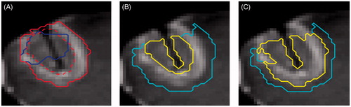
The region of contrast enhancement was segmented manually (Amira 5.4.2, FEI, Hillsboro, OR) using pre-treatment subtraction images to delineate the gross tumour volume. On post-treatment subtraction images, the non-enhancing central region and enhancing ring were segmented to define the thermal ablation lesion (Figure 1). The registered T1-weighted images and segmentations were then resampled (“WarpImageMultiTransform”, Advanced Neuroimaging Tools (ANTs) [34]) into the 2 D geometry of the MRTI acquisition so that temperature histories could be linked to the segmentation data on a per pixel basis (Figure 1(A)). After resampling, the outer edge of the enhancing ring was dilated using a 5 × 5 kernel (≈5 mm) to define an outer non-enhancing region where there was temperature increase but no radiologic change.

Figure 1. Tumour/thermal lesion segmentations and predicted regions. The segmented tumour (blue) and the thermal lesion defined by the central non-enhancing region (red dotted) and enhancing ring (red solid) with skull-stripped post-treatment post-contrast image in the background (A). The regions classified as y = 1 (yellow) and y = 0 (cyan) for the inner boundary (B), outer boundary (C) predictions with skull-stripped post-treatment post-contrast image in the background. The area adjacent to the skull has been excluded due to uncertainty in the segmentation and the area of ambiguous enhancement was excluded in the outer boundary model (C).

Arrhenius parameter optimisation

The resampled segmentation data was used to assign each temperature history a binary classification () that reflects its post-treatment radiologic appearance. These classifications were used in a binary logistic regression that gives the probability of observing a specific post-treatment appearance, , as a function of the fractional conversion: (6) where FC₅₀ is the fractional conversion and k₅₀ is the slope when . The optimal Arrhenius parameters were defined to be the pair of E_a and A values that maximise the joint log likelihood of this coupled AR–logistic model.

Rosenberg [35], Wright [36] and He and Bischof [37,38] have previously measured a linear correlation between E_a and log(A) for variety of thermally sensitive biological processes. Regardless of whether this correlation is a consequence of a thermodynamic compensation law or an artefact of the fitting process [39–43], it restricts the possible parameter pairs in the E_a/log(A) parameter space to a line within some experimental tolerance. In this work, we assume the relationship measured by He and Bischof: (7)

A re-parametrised form of Equation (1)(1) was used during optimisation that utilises a transformed set of Arrhenius parameters, E_a and log(A_Ref) to effectively focus the parameter search on values near this line. This approach facilitates the convergence of the optimisation algorithm and aids in visualising of the solutions [44,45]. The mathematical details of this re-parameterisation are given in Appendix A.1. The optimisations were solved using a quasi-Newton BFGS algorithm (fminunc, MATALB R2015a, Mathworks, Natick, MA) with the Arrhenius parameters reported by Henriques [10] as the initial guess. The approximate Hessian at the solution was inverted to estimate the covariance matrix and generate confidence ellipses for the solution. The solutions and covariance matrices were then transformed into the original E_a/log(A) parameter space for comparison with parameters found in the literature.

Inner/outer boundary modelling

For post-treatment contrast-enhanced imaging the radiologic features of interest are the boundaries between the central non-enhancing region and the enhancing ring (inner boundary) and the enhancing ring and the outer non-enhancing region (outer boundary). The optimal set of model parameters that characterise the inner ring boundary was found by assigning all pixels in the central non-enhancing region y = 1 and all pixels in the enhancing ring and outer non-enhancing region y = 0 and applying the technique described in the previous section. Similarly, a set of parameters were found for the outer boundary by assigning all pixels in the central non-enhancing region and enhancing ring y = 1 and those in the outer non-enhancing region y = 0. Pixels that enhanced on both pre- and post-treatment subtraction images were excluded from the outer boundary optimisation, since it is ambiguous whether their enhancement is due to treatment effect or residual tumour. Data in these regions would be inappropriate for training as the logistic regression demands we know the fraction of damaged tissue and no assumptions can be made in these areas. Additionally, regions of low signal at the skull–brain interface and at the position of the laser were excluded from training to avoid biasing the results. A representative example of the pixel assignments and excluded areas is shown in Figure 1.

Temperature histories for each patient were grouped together to generate patient averaged parameters for the inner/outer boundaries with optimal dose thresholds chosen to minimise the sum of false positives and false negatives. The inner and outer boundary parameters were fit using 4810 and 4337 pixels, respectively. The Arrhenius parameters of both of these boundaries were compared to seven values from the literature (Table 1). In the special case of the CEM_SD, Equations (4)(4) and (7)(7) were used to calculate the Arrhenius parameters at high temperatures ( to reflect the effective parameters used in the literature. The inner and outer boundary Arrhenius parameters were also used to calculate the equivalent R_CEM using Equation (4)(4) . Optimal dose thresholds were also calculated for the CEM_SD model (CEM_SD-thresh) and the maximum temperature (T_c) for direct comparison to previous work in the literature.

Table 1. Selected Arrhenius parameters from literature.

Study	Log frequency factor log(A)	Activation energy EA  [kJ/mol]	Isoeffect
Henriques† [10]	227	628	Second degree burns; porcine skin (in vivo)
CEMSD*,† [11]	210	578	Various (in vivo/ex vivo) [50]
Qin [30]	64.2	189	Protein denaturation; whole cells; DSC with Tmax = 60 °C
Qin [30]	145	401	Protein denaturation; whole cells; DSC with Tmax = 50 °C
Jacques‡ [26]	87.2	258	Optical scattering coefficient; porcine liver (ex vivo)
Borelli‡ [24]	185	506	Cell survival; baby hamster kidney cells
Brown‡ [27]	245	667	Microvasculature disruption; murine muscle (in vivo)

† Used in FDA cleared ablation system.

* Calculated assuming R = 0.5 and Equations (4)(4) and (7)(7) .

‡ Associated with inner/outer ring boundaries on T2-weighted imaging by Sherar et al. [16].

The model predicted regions, A_model, were calculated for each ablation and compared to the segmented regions, A_seg, to get a practical measure of the goodness of fit using three quantitative measures of agreement. The first is the Dice Similarity Coefficient (DSC), which is a measure of the spatial overlap of two regions where a value of 1 corresponds to complete overlap and a value of 0 corresponds to no overlap. While the DSC is commonly used in radiology research, its value is biased by the centre of the lesion which is virtually guaranteed to match assuming the areas are properly registered. For this reason, two additional measures of agreement based on the distances between the modelled and segmented boundaries were also calculated: the Hausdorff distance (HD) and the mean distance to agreement (MDA). The HD represents the largest difference between two boundaries and can be considered a measure of the worst-case scenario disagreement. However, as a maximum value it is inherently sensitive to noise and outliers. The MDA is a measure of the average distance between the two boundaries. Both the HD and MDA have units of distance so they can be intuitively interpreted in the context of the overall lesion size and voxel size. Taken together, these three measures of agreement give a more complete picture of model parameter performance. The mathematical definition of each can be found in Appendix A.2.

After comparing the predicted inner and outer boundary regions to the segmented regions they were compared to the two dose model implementations used in FDA cleared laser ablation systems (AR_Henriques; Ω = 1 [8] and CEM_SD = 2, 10, 60 min [9]). An additional threshold of CEM_SD=240 min was included because it is commonly used as upper limit for damage in ablation literature [46].

Results

Arrhenius parameter optimisation

To evaluate the convergence of the optimisation algorithm the negative log likelihood was calculated over the range of log(A_Ref)/E_A  values commonly found in the literature. For each optimisation, there is a single local minimum where the surface is smooth and convex. These solutions and 95% confidence ellipses are plotted in the log(A_Ref)/E_A  reference space along with selected literature values for comparison in Figure 2(A,B). The axis limits in this Figure 2 were deliberately chosen to represent the upper limits of the values observed in the literature. The advantages of the re-parameterisation in Equation (7)(7) are apparent when the same data are plotted in the traditional log(A)/E_A  space (Figure 2(C)). The high correlation between parameters causes the confidence ellipses to appear as lines and makes visual comparison using the confidence regions and literature values nearly impossible. The confidence ellipses do not overlap, suggesting that they are two distinct solutions and that the differing values are not a statistical consequence of the compensation law. The parameters that define these ellipses are given in Table 2.

Figure 2. Optimal Arrhenius parameters. The optimal Arrhenius parameters (green circle) and 95% confidence regions (green) are shown with the negative log likelihood in the background in the log(A_Ref)/E_A  parameter space for the inner boundary (A) and outer boundary (B) model parameters. The same data is shown in the log(A)/E_A  parameter space (C). The Arrhenius parameters (magenta) from Henriques (♦), CEM (•), Qin (T_max = 60 °C;▲), Qin (T_max = 50 °C;▼), Jacques (*), Borelli (▪) and Brown (⋆). The empirical linear relationship between E_A  and log(A) (black dotted) is also plotted for reference.

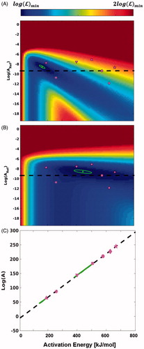
Table 2. Optimal model parameters and 95% confidence ellipses.

	Inner boundary model	Outer boundary model
Activation energy, EA  [kJ/mol]	162	445
Log frequency factor, log(A) [s^−1]	53.0	161
Minor axis length	0.187	0.251
Major axis length	20.78	65.4
Slope [kJ^−1]	0.366	0.376
Intercept	−6.25	−6.99
RCEM	0.82	0.59

Table 3. Optimal logit parameters and thresholds for the inner and outer boundary models.

	Inner boundary model	Outer boundary model
k	7.80	7.11
FC50	0.61	0.26
AR model thresholds ()	0.54/0.63/0.99	0.40/0.20/0.22

Optimal dose model parameters

The Arrhenius parameter values that define the inner boundary are lower than those of the outer boundary and span activation energies from 142 kJ/mol to 182 kJ/mol. They do not overlap with any of the model parameters from the literature but are closest to the coefficients reported by Jacques and Qin (T_max = 60°C). These coefficients correspond to a R_CEM value of 0.82. The outer boundary model parameters have higher coefficient values that span activation energies of 384 kJ/mol to 506 kJ/mol. Like the inner boundary model parameters, these coefficients do not overlap with any of those found in the literature, but they are closest to coefficients of the CEM, Qin (T_max = 50°C), and Borrelli model parameters. The activation energy of the Borelli and Qin (T_max = 50°C) model parameters is consistent with the values of the outer boundary model parameters, but a difference in the frequency factor prevents it from overlapping with the confidence ellipse. These coefficients correspond to equivalent R_CEM value of 0.59. For both solutions, the confidence ellipses imply a linear relationship between log(A) and E_A with slopes and intercepts that are larger than used in Equation (7)(7) (Table 2).

Optimal dose thresholds

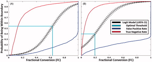
Figure 3 shows the probability of being within the respective boundary as a function of FC along with the thresholds that optimise accuracy. The optimal threshold for the inner boundary model parameters corresponds to a thermal dose of Ω = 0.99/FC = 0.63. This threshold is coincidentally effectively equal to the historically used threshold of Ω = 1. The optimal threshold for the outer boundary model parameters is a thermal dose of Ω = 0.22/FC = 0.20 (Table 3). Both models performed extremely well, with areas under the curve and accuracy in excess of 95% and 85%, respectively. The values of CEM_SD-thresh were 1.8 × 10⁵ min and 32 min for the inner and outer boundaries, respectively while T_c was found to be 61.5 °C and 47.6 °C for the inner and outer boundaries, respectively.

Figure 3. Inner and outer boundary models. The probability of being contained within the inner (A) and outer boundary (B) as a function of fractional conversion using the optimal Arrhenius parameters in Table 1. The threshold that maximises the accuracy is shown in cyan. The false-positive (blue) and true-negative rates (red) are shown for reference.

Model predicted region comparison

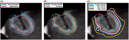
Figure 4 shows a representative comparison between the areas predicted using the inner/outer boundary model parameters and the segmentations (a), AR_Henriques (b) and CEM_SD (c) for 4 dose thresholds. The mean DSC/DTA/HD between the predicted boundaries and segmentations was 0.87/0.93 mm/2.92 mm and 0.89/1.1 mm/3.5 mm for the inner and outer boundary, respectively. In both cases, the mean DTA is on the order of the pixel size (1 mm). There is consistent disagreement at the edge of the skull in Figure 4(A) that is likely caused by partial voluming which underscores the need to remove selected areas from fitting. On average, the region predicted by AR_Henriques fell between the predicted inner and outer ring boundaries with a MDA of 1.5 mm from each boundary. The CEM_SD threshold of 60 min practically indistinguishable from the outer ring model with a DSC/DTA/HD of 0.98/0.24 mm/0.99 mm. The 240 and 10 min thresholds were just inside and outside the outer boundary model and agreed within a pixel size with a DSC/DTA/HD of 0.91/0.84 mm/2.17 mm and 0.92/0.88 mm/2.93 mm, respectively. The AR_Jacques, AR_Borelli, AR_Brown predictions show excellent agreement with the outer and inner boundaries as previously investigated by Sherar et al. with DSC/DTA/HD = >0.96/<0.38 mm/<1.22 mm [16].

Figure 4. Isodose line comparisons. The predicted inner and outer boundary regions are compared to the inner and outer boundary segmentations (A), AR_Henriques prediction (B) and CEM_SD prediction (C).

Discussion

The combination of temperature and thermal dose monitoring is an increasingly important tool that enables adaptive changes during select thermal therapies to maximise therapeutic effect. However, the dose model parameters that underlie these models only approximate the complex physiologic processes that occur in the thermal lesion. This contrasts with the clinical reality where post-treatment imaging serves as the gold–standard endpoint for treatment evaluation. Therefore, it is of interest to develop a technique for deriving dose model parameters directly from post-treatment imaging that are predictive of the kinetics that underlie specific radiologic changes. This approach makes it possible to leverage available clinical data for procedure specific dose modelling and continued investigation into its clinical utility.

In this work, we have established the feasibility of deriving thermal dose model parameters directly from post-treatment imaging through retrospective analysis of laser ablation procedures. The technical challenges typically associated with this type of measurement were overcome by developing a non-linear optimisation technique for solving a coupled AR-logistic model for the model parameters that define the inner and outer boundaries of the characteristic enhancing ring on post-treatment contrast-enhanced T1-weighted imaging in human brain. Each optimisation converged to a unique solution that is within with range of parameters reported for a variety of biological processes. While this indicates technical success in converging on a physically plausible solution, the feasibility of the technique is best understood through critical comparison with similar investigations in the literature and previous clinical experience.

The majority of previous in vivo studies have focussed on using the CEM and CT dose models to find threshold doses that best correlate with imaging features of interest for various experimental conditions [9,13,14,17,47,48] where the most appropriate comparison is outer boundary model. A similar analysis was performed in this work to obtain CEM_SD-thresh and T_c (32 min/47.6 °C for outer boundary model), which are consistent with the approximate ranges found in the literature (∼10°–10³ min/48–60 °C for outer boundary). One study that specifically examined the inner boundary quoted a threshold dose of 10⁹ min for the CEM model [16]. While this differs from our result of 1.8 × 10⁵ min by several orders of magnitude, this disagreement can be attributed to the inherent uncertainty that results from the exponential nature of the CEM model when applied at high temperatures.

The values of the underlying Arrhenius parameters also compare favourably to similar investigations using the AR model. Sherar et al. [16] correlated the areas predicted by three previously published sets of model parameters with the inner and outer boundaries of the hyperintense ring on T2-weighted imaging in rabbit brain. They found that the model parameters published by Jacques [26] correlated well with the inner boundary, while the Brown [27] and Borelli [24] model parameters correlated well with the outer boundary which is consistent with the values found in this study. In a separate study, Qin et al. [30] examined the effective activation energies of protein denaturation in four different cells lines using dynamic scanning calorimetry (DSC) at different maximum temperatures. Their results at T_max = 60 °C and T_max = 50 °C  provide the best comparison to the activation energies for the inner and outer boundary models if the critical temperatures, T_c, from this study (61.5 °C and 47.6 °C) are considered to be surrogates for the DSC end temperature. When their results are averaged over the four different cell lines for T_max = 60 °C and T_max = 50 °C  (189 kJ and 401 kJ), they compare favourably to the range of activation energies found in this study for the inner and outer boundary models (142–182 kJ and 384–506 kJ) (Figure 2). This also suggests that post-treatment contrast-enhanced imaging may be an appropriate surrogate for the denaturation of major cellular proteins. The existence of two distinct solutions for each boundary is notable since implies that the effective kinetics that underlie the formation of each boundary are also distinct. Consequently, these kinetic parameters result in R_CEM values (0.82 and 0.59 for inner and outer boundary model, respectively) that are distinct from the ubiquitous Sapareto and Dewey parameters ( and are consistent with the observations of Dewhirst [49]. This suggests further investigation of endpoint-specific dose model parameters is warranted.

While comparison of model parameters and optimal dose thresholds support the theoretical aspects of this work, the evaluation of the areas enclosed by the inner and outer boundaries provide a more practical and intuitive comparison. Comparing the model predicted regions to segmented regions serves as a measure of the goodness of fit. While some measurable disagreement is observed visually and via the DSC and HD metrics, the average disagreement measured using the DTA metric (0.93 mm and 1.1 mm for the inner and outer boundary model, respectively) was on the order of the imaging resolution (1 mm). The Henriques and CEM dose models parameters/thresholds provide a meaningful point of comparison, because they are used clinically for this particular procedure. Thus, the modest differences (<1 mm) observed when comparing these models to the inner and outer boundary model show our results are consistent with clinical experience. It is important to note that the ablations examined in this work are characterised by high spatial temperature gradients which results in CEM thresholds that overlap for practical purposes. Thus, the choice of parameters would have a marginal impact on the size of the lesions in these particular procedures. However, the technique described here provides two major theoretical advantages in the context of the larger variety of available ablation procedures. First, the AR logistic approach solves for the underlying kinetic parameters that can cause measurable and consistent differences in lesion size even in these high-temperature short-duration procedures. This is shown by the consistent difference observed between the AR_Henriques and CEM_SD predictions. Second, AR-logistic approach allows interpretation of dose values in terms of a probability of observing the specified radiologic feature (Figure 3) with confidence defined by ROC metrics rather than only obtaining a single-dose threshold. This provides a more intuitive approach to interpreting dose while utilising a quantity that does not increase arbitrarily towards infinity. Both of these aspects of the AR-logistic technique are expected to become substantial when applied to procedures performed at lower temperatures and longer durations and the transition from native to damaged tissue is more gradual.

The primary limitations of this study were its retrospective nature and the limited number of patients (N = 5). Training and validation sets or cross-validation techniques were not feasible with this limited data, and consequently, the predictive value of the resulting models cannot be properly evaluated. However, the objective was not to derive definitive parameters for the appearance of the thermal lesion but rather to rigorously describe and demonstrate a technique is technically possible by demonstrating agreement with previous studies. The limited number of patients also meant that all clinical indications were included in the parameter fitting so that differences between the melanoma and breast metastases, for example, could not be ascertained. However, this initial study establishes a new technique that can be used to derive dose parameter values directly from clinical data which enables future work focussed on developing prospective studies that examine the impact of this approach on different procedures, clinical indications and radiologic endpoints.

The AR-logistic methodology was developed as a practical approach to clinical reality where the only available endpoints are radiologic in nature. Thus, the focus is primarily on reconciling dose feedback with the post-treatment changes observed by the treating physicians. This implicitly relies on the assumption that imaging accurately reflects the physiology of the development of thermal lesions on a tissue and cellular level which is an area of ongoing research. Although impractical and unethical in human subjects, this method could theoretically be extended to use in animal studies where histological analysis can be incorporated to further study the connection between thermal dose, physiology and diagnostic imaging. Ultimately, these types of studies could be critical for answering these fundamental physiologic questions and inform the selection of optimal dose models for translation to the clinic.

Conclusions

This work establishes the feasibility of establishing patient-derived thermal dose model parameters through retrospective correlation of intraoperative MR data acquired during thermal ablation procedures with post-treatment imaging radiologic effects. This is decidedly different methodology compared to previous studies which are restricted to laboratory experiments. The approach enables investigation and development of procedure specific thermal dose models that can be refined as with increasing clinical experience. Expanded prospective investigations in a larger cohort of patients is needed to validate the technique as well as investigate models based on other post-treatment imaging effects which are candidates to act as surrogate markers for specific responses to therapy.

Disclosure statement

No potential conflict of interest was reported by the authors.

Additional information

Funding

National Center for Advancing Translational Sciences10.13039/100006108TL1TR000369UL1TR000371This work was supported by the National Center for Advancing Translational Sciences of the National Institutes of Health [TL1TR000369 and UL1TR000371].

Appendix A

A.1 Re-parameterised AR model equation

Equation (1)(1) was re-parameterised [44] by including an additional parameter called the reference temperature, T_Ref, (A1.1) where (A1.2)

T_Ref was chosen to be equal to 316.5 °K to remove the correlation implied by Equation (7)(7) . This results in a transformed set of Arrhenius parameters, A_Ref and E_A, that are approximately orthogonal and facilitates optimisation.

A.2 Region comparisons

Three quantitative methods of comparison were used to compare the segmented and model predicted areas. The first is the Dice Similarity Coefficient (DSC): (A2.1)

In general, for two boundaries defined as sets of Cartesian coordinates, and , the quantity (A2.2) represents the minimum Euclidean distance from between every point on boundary A and any point on boundary B. Note that is not communitive (). The HD is defined as follows: (A2.3) which is the maximum value of d found in and . The mean distance to agreement (MDA): (A2.4) where n and m are the number of points that define boundary A and B, respectively.

References

- Carpentier A, Itzcovitz J, Payen D, et al. (2008). Real-time magnetic resonance guided laser thermal therapy for focal metastatic brain tumors. Neurosurgery 63:ONS21–9.
- Medvid R, Ruiz A, Komotar RJ, et al. (2015). Current applications of MRI-guided laser interstitial thermal therapy in the treatment of brain neoplasms and epilepsy: a radiologic and neurosurgical overview. Am J Neuroradiol 36:1998–2006.
- Jethwa PR, Barrese JC, Gowda A, et al. (2012). Magnetic resonance thermometry-guided laser-induced thermal therapy for intracranial neoplasms: initial experience. Oper Neurosurg 71:133–45.
- Hawasli AH, Bagade S, Shimony JS, et al. (2013). Magnetic resonance imaging-guided focused laser interstitial thermal therapy for intracranial lesions: single-institution series. Neurosurgery 73:1007–17.
- Missios S, Bekelis K, Barnett GH. (2015). Renaissance of laser interstitial thermal ablation. Neurosurg Focus 38:E13.
- Mohammadi AM, Hawasli AH, Rodriguez A, et al. (2014). The role of laser interstitial thermal therapy in enhancing progression-free survival of difficult-to-access high-grade gliomas: a multicenter study. Cancer Med 3:971–9.
- Tatsui CE, Stafford RJ, Li J, et al. (2015). Utilization of laser interstitial thermotherapy guided by real-time thermal MRI as an alternative to separation surgery in the management of spinal metastasis. J Neurosurg Spine 23:400–11.
- McNichols RJ, Gowda A, Kangasniemi M, et al. (2004). MR thermometry-based feedback control of laser interstitial thermal therapy at 980 nm. Lasers Surg Med 34:48–55.
- Sloan AE, Ahluwalia MS, Valerio-Pascua J, et al. (2013). Results of the NeuroBlate System first-in-humans phase I clinical trial for recurrent glioblastoma: clinical article. J Neurosurg 118:1202–19.
- Henriques FC. Jr. (1947). Studies of thermal injury. V. The predictability and the significance of thermally induced rate processes leading to irreversible epidermal injury. Arch Pathol 43:489–502.
- Sapareto SA, Dewey WC. (1984). Thermal dose determination in cancer therapy. Int J Radiat Oncol Biol Phys 10:787–800.
- Rempp H, Hoffmann R, Roland J, et al. (2011). Threshold-based prediction of the coagulation zone in sequential temperature mapping in MR-guided radiofrequency ablation of liver tumours. Eur Radiol 22:1091–100.
- McDannold NJ, King RL, Jolesz FA, et al. (2000). Usefulness of MR imaging-derived thermometry and dosimetry in determining the threshold for tissue damage induced by thermal surgery in rabbits. Radiology 216:517–23.
- Peters RD, Chan E, Trachtenberg J, et al. (2000). Magnetic resonance thermometry for predicting thermal damage: An application of interstitial laser coagulation in an in vivo canine prostate model. Magn Reson Med 44:873–83.
- Kickhefel A, Rosenberg C, Weiss CR, et al. (2011). Clinical evaluation of MR temperature monitoring of laser-induced thermotherapy in human liver using the proton-resonance-frequency method and predictive models of cell death. J Magn Reson Imaging 33:704–9.
- Sherar MD, Moriarty JA, Kolios MC, et al. (2000). Comparison of thermal damage calculated using magnetic resonance thermometry, with magnetic resonance imaging post-treatment and histology, after interstitial microwave thermal therapy of rabbit brain. Phys Med Biol 45:3563.
- Chen L, Wansapura JP, Heit G, et al. (2002). Study of laser ablation in the in vivo rabbit brain with MR thermometry. J Magn Reson Imaging 16:147–52.
- Fahrenholtz SJ, Moon TY, Franco M, et al. (2015). A model evaluation study for treatment planning of laser-induced thermal therapy. Int J Hyperthermia 31:705–14.
- Hectors SJCG, Jacobs I, Moonen CTW, et al. (2016). MRI methods for the evaluation of high intensity focused ultrasound tumor treatment: current status and future needs. Magn Reson Med 75:302–17.
- Pearce JA. (2013). Comparative analysis of mathematical models of cell death and thermal damage processes. Int J Hyperthermia Group 29:262–80.
- Chung AH, Jolesz FA, Hynynen K. (1999). Thermal dosimetry of a focused ultrasound beam in vivo by magnetic resonance imaging. Med Phys 26:2017–26.
- Hazle JD, Diederich CJ, Kangasniemi M, et al. (2002). MRI-guided thermal therapy of transplanted tumors in the canine prostate using a directional transurethral ultrasound applicator. J Magn Reson Imaging 15:409–17.
- Hazle JD, Stafford RJ, Price RE. (2002). Magnetic resonance imaging-guided focused ultrasound thermal therapy in experimental animal models: correlation of ablation volumes with pathology in rabbit muscle and VX2 tumors. J Magn Reson Imaging 15:185–94.
- Borrelli MJ, Thompson LL, Cain CA, et al. (1990). Time-temperature analysis of cell killing of BHK cells heated at temperatures in the range of 43.5 °C to 57.0 °C. Int J Radiat Oncol 19:389–99.
- Moritz AR, Henriques FC. (1947). Studies of thermal injury: II. The relative importance of time and surface temperature in the causation of cutaneous burns. Am J Pathol 23:695–720.
- Jacques S, Newman C, He XY, Thermal coagulation of tissues. Liver studies indicate a distribution of rate parameters, not a single rate parameter, describes the coagulation process. Am Soc Mech Eng Heat Transf Div Publ HTD. Atlanta (GA): ASME; 1991.
- Brown SL, Hunt JW, Hill RP. (1992). Differential thermal sensitivity of tumour and normal tissue microvascular response during hyperthermia. Int J Hyperth Off J Eur Soc Hyperthermic Oncol North Am Hyperth Group 8:501–14.
- Miles CA, Bailey AJ. (2004). Studies of the collagen-like peptide (Pro-Pro-Gly)(10) confirm that the shape and position of the type I collagen denaturation endotherm is governed by the rate of helix unfolding. J Mol Biol 337:917–31.
- Miles CA. (2007). Kinetics of the helix/coil transition of the collagen-like peptide (Pro-Hyp-Gly)(10). Biopolymers 87:51–67.
- Qin Z, Balasubramanian SK, Wolkers WF, et al. (2014). Correlated parameter fit of Arrhenius model for thermal denaturation of proteins and cells. Ann Biomed Eng 42:2392–404.
- He X, Wolkers WF, Crowe JH, et al. (2004). In situ thermal denaturation of proteins in dunning AT-1 prostate cancer cells: implication for hyperthermic cell injury. Ann Biomed Eng 32:1384–98.
- McDannold N. (2005). Quantitative MRI-based temperature mapping based on the proton resonant frequency shift: review of validation studies. Int J Hyperthermia 21:533–46.
- Smith SM. (2002). Fast robust automated brain extraction. Hum Brain Mapp 17:143–55.
- Avants BB, Tustison NJ, Song G, et al. (2011). A reproducible evaluation of ANTs similarity metric performance in brain image registration. NeuroImage 54:2033–44.
- Rosenberg B, Kemeny G, Switzer RC, et al. (1971). Quantitative evidence for protein denaturation as the cause of thermal death. Nature 232:471–3.
- Wright NT. (2003). On a relationship between the Arrhenius parameters from thermal damage studies. J Biomech Eng 125:300–4.
- He X, Bischof JC. (2003). Quantification of temperature and injury response in thermal therapy and cryosurgery. Crit Rev Biomed Eng 31:355–422.
- He X, Bhowmick S, Bischof JC. (2009). Thermal therapy in urologic systems: a comparison of arrhenius and thermal isoeffective dose models in predicting hyperthermic injury. J Biomech Eng 131:074507.
- Sharp K. (2001). Entropy-enthalpy compensation: fact or artifact? Protein Sci 10:661–7.
- Liu L, Guo Q-X. (2001). Isokinetic relationship, isoequilibrium relationship, and enthalpy-entropy compensation. Chem Rev 101:673–96.
- Krug RR, Hunter WG, Grieger RA. (1976). Enthalpy-entropy compensation. 1. Some fundamental statistical problems associated with the analysis of van’t Hoff and Arrhenius data. J Phys Chem 80:2335–41.
- Barrie PJ. (2012). The mathematical origins of the kinetic compensation effect: 1. The effect of random experimental errors. Phys Chem Chem Phys 14:318–26.
- Barrie PJ. (2012). The mathematical origins of the kinetic compensation effect: 2. The effect of systematic errors. Phys Chem Chem Phys 14:327–36.
- Schwaab M, Pinto JC. (2007). Optimum reference temperature for reparameterization of the Arrhenius equation. Part 1: problems involving one kinetic constant. Chem Eng Sci 62:2750–64.
- Schwaab M, Lemos LP, Pinto JC. (2008). Optimum reference temperature for reparameterization of the Arrhenius equation. Part 2: problems involving multiple reparameterizations. Chem Eng Sci 63:2895–906.
- Damianou CA, Hynynen K, Fan X. (1995). Evaluation of accuracy of a theoretical model for predicting the necrosed tissue volume during focused ultrasound surgery. IEEE Trans Ultrason Ferroelectr Freq Control 42:182–7.
- Yung JP, Shetty A, Elliott A, et al. (2010). Quantitative comparison of thermal dose models in normal canine brain. Med Phys 37:5313–21.
- McDannold N, Vykhodtseva N, Jolesz FA, et al. (2004). MRI investigation of the threshold for thermally induced blood–brain barrier disruption and brain tissue damage in the rabbit brain. Magn Reson Med 51:913–23.
- Dewhirst MW, Viglianti BL, Lora-Michiels M, et al. (2003). Basic principles of thermal dosimetry and thermal thresholds for tissue damage from hyperthermia. Int J Hyperthermia 19:267–94.
- Dewey WC, Hopwood LE, Sapareto SA, et al. (1977). Cellular responses to combinations of hyperthermia and radiation. Radiology 123:463–74.