An MR-compatible antenna and application in a murine superficial hyperthermia applicator

Abstract

In this work, a novel magnetic resonance (MR)-compatible microwave antenna was designed and validated in a small animal superficial hyperthermia applicator. The antenna operates at 2.45 GHz and matching is made robust against production and setup inaccuracies. To validate our theoretical concept, a prototype of the applicator was manufactured and tested for its properties concerning input reflection, sensitivity for setup inaccuracies, environment temperature stability and MR-compatibility. The experiments show that the applicator indeed fulfils the requirements for MR-guided hyperthermia investigation in small animals: it creates a small heating focus (<1 cm³), has a stable and reliable performance (S₁₁< −15 dB) for all working conditions and is MR-compatible.

Keywords:

• Hyperthermia antenna
• MR-compatibility
• microwave applicator
• small animal heating systems

Introduction

Hyperthermia (HT), locally heating tissues to 41–43 °C, is known as a potent sensitiser of radio- and chemotherapy in cancer treatment without adding severe side effects [1–4]. Novel treatment procedures of radiotherapy and chemotherapy in combination with HT are under investigation [5]. Successful clinical introduction of new treatment combinations is enhanced by experimental in vivo studies using anthropomorphic murine models. Such studies require a dedicated applicator for local heating, especially for the head and neck (H&N) region. Magnetic resonance (MR)-compatibility is desired for precise 3D thermal dosimetry and real-time assessment of tumour physiology by MR imaging. Hence, a dedicated murine HT applicator for the H&N is required.

The current method to perform animal studies on HT effects in the H&N region involves placing and heating neck tissue tumours on the leg of a small rodent. This has two main issues. Firstly, the rodent’s leg is not the location where these tumours originate, affecting their growth, molecular and physiological behaviour. Secondly, heating is performed by submerging the leg in a hot water bath, affecting the entire leg instead of the tumour tissue only [6]. It is generally assumed that research using orthotopic tumour models, in which the tumour is embedded within its natural environment, and in which only the tumour is heated, are more representative for the clinical situation [7].

Existing examples of animal devices with the ability to heat locally, are based on radiofrequency (RF) (waveguides) [8], ultrasound [9,10] and laser-based phototherapy [11]. These solutions fail in the H&N and/or rely on invasive probes to measure temperature, disrupting tissues and local microenvironment and causing discomfort for the animal. Our approach was built on the requirement of local heating in the H&N and operation in a 7T MRI scanner (Agilent, Santa Clara, CA, USA), to apply MR imaging for setup verification, thermometry and tumour response monitoring.

This publication was solicited by the chief editor as follow-up of an ICHO 2016 young investigator award [12]. It presents a novel antenna design that allows superficial (this article) and deep (further study) HT under MR-control. Our concept is based on an MR-transparent Yagi–Uda antenna that was designed for the human H&N region [13]. This design was modified by applying embedded feed lines to make the antenna robust to construction tolerances, which are more prominent at 2.45 GHz compared to our previous work at 433 MHz. The target animal is placed on top of a so-called water bolus, in which the antenna is embedded for optimal matching and cooling. The design of the water bolus and antenna scaffold are included in this research, as well as the experimental validation of the heating pattern for single-antenna operation and the MR-compatibility of the single-antenna set-up.

Material and methods

Requirements

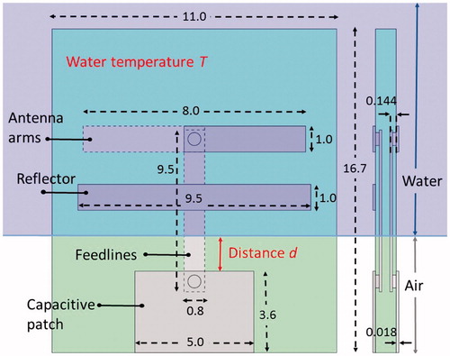
The antenna input reflection coefficient (S₁₁)-design requirement was set to less than −15 dB, i.e. <3% reflection of the power to the power amplifier, to avoid overloading the power source. The antenna should be matched to 50 Ω in air at the connection side of the power source (bottom in Figure 1), while on the other end the antenna was designed for operation in water (radiating part or antenna arms, top in Figure 1). Hence, an air–water boundary is inevitable, since the connector cannot be immersed in water. This influences the performance of the antenna, especially at frequencies >1 GHz. In addition, the antenna must be robust for differences in water temperature, which affects antenna impedance matching [14,15].

Figure 1. Antenna blueprint with distances in millimetre. Distance (d) and water temperature (T) are varied in the experiments. Distance (d) is varied by changing the distance that the antenna protrudes into the water-filled container (purple region).

The xenograft H&N tumours in mice are anticipated to be ∼80 mm³ in size. The ISM (industrial, scientific and medical) license-free bands at 915 MHz, 2.45 GHz and 5.80 GHz were each tested in simulations in SEMCAD¹. The finite-difference time-domain (FDTD) implementation was used. Muscle properties were used for the target (muscle properties derived from [7]) to estimate the size of the specific absorption rate (SAR) distribution at each frequency. The ISM license-free frequency of 2.45 GHz was chosen as operating frequency of the antenna, because the size of the SAR distribution was closest to the expected tumour size of 80 mm³.

To ensure MR-compatibility, the antenna layers were designed for a minimal cross-section in the direction of the main magnetic field and the RF fields of the MR-scanner. The antenna was produced as a printed circuit board (PCB) because this production method enables the reproducible development of very thin metal layers and hence a very small cross section is required for maximum MR transparency. An overview of the design criteria is given in Table 1.

Table 1. Design specifications and constraints for the development of the antenna.

Property	Constraint
S11	≤−15 dB
Matching	50 Ω
Frequency	2.45 GHz
S11 for changing air–water boundary	≤−15 dB
S11 for changing water temperature	≤−15 dB
Technology	PCB
MR-compatible	Yes

Antenna design

The FDTD implementation in SEMCAD and its successor Sim4Life² were used for the design of the antenna and the HT applicator. The metal within the antenna was modelled as a perfect electric conductor (PEC) to increase simulation speed. Air was modelled using vacuum properties. The PCB board material was modelled with FR-4 material properties [16], i.e. a relative permittivity of 4.2. A grid of 1.9 MCells was employed with a minimum step size of 6.0 µm (in thin metal layers) and maximum step of 7.6 mm (in FR4). Strong absorbing boundary conditions (absorption ≥99.9%) were used in every direction around the antenna at a distance of 10 mm. This relatively close distance is motivated by the fact that the antenna operates in a very lossy environment.

The antenna was based on an earlier designed Yagi–Uda arrangement [13]. To prevent power losses due to reflections at the point where the feed lines cross the air–water interface (Figure 1), the feed lines were embedded within the PCB. As a result, the feed lines are completely shielded from the air–water interface, making the antenna stable for changing distance d (see Figure 1). A capacitive patch at the bottom of the antenna ensures matching to 50 Ω and provides an attachment point for a MMCX connector.

The input return loss (S₁₁) was measured to verify how well the antenna is matched to 50 Ω for varying water temperatures (33–43 °C) at a water level (d) of 3.0 mm (Figure 1). In addition, we measured the antenna impedance performance for varying water levels (d = 0.1–4 mm) at a water temperature (T) of 37 °C. The antenna input return loss was measured with a ZNC3 Rohde&Schwarz Vector Network Analyser (Rohde&Schwarz, Munich, Germany), calibrated with a ZCAN N-port 50 Ω calibration set.

Water bolus and scaffold design

The water in the water bolus was modelled as demineralised water according to a Debye dispersion model [17]. For the antenna design, dielectric properties for demineralised water at 37 °C were used. This relatively high temperature is required to counteract the decrease of animal body temperature under sedation [18,19]. Water was assumed to be circulating to cool the antenna and the animal’s skin and to stabilise the temperature in the applicator. Therefore, mixed boundary conditions for heat transfer between the water and the animal were assumed in the model. Note that the contact surface between the animal, in our experiments modelled by a phantom (Figure 2), and the water bolus has a major influence on the actual heat transfer between these objects. The water bolus is designed to surround the animal with water to the height of at least the flanks. The 3D-printed scaffold (PA 2200) holds the antenna as well as the water bolus and provides connections for the water supply.

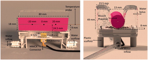
Figure 2. Applicator with embedded antenna, water bolus and animal placeholder in Experiment 1. Note that the animal mimicking phantom in Experiment 2 was positioned 4 mm lower and had a 20 mm diameter. The black dots in the left picture mark temperature sensor locations.

Experiment 1: Heating performance

A phantom was heated with the applicator while the temperature was monitored at three locations within the phantom (see Figure 2). A Kuhne KU SG 2.45–25 A signal generator(Kuhne Electronic GmbH, Berg, Germany) was used to provide a 2.45 GHz signal with a power of 17.4 W at the connector of the antenna for 6 min. Due to reflections in the connector and antenna mismatch, 16.5 W was estimated to be transferred to the antenna arms. The signal generator was connected to the antenna with a RG316 cable.

The phantoms used were agar-based and produced to have a permittivity and conductivity equal to those of muscle tissue [20]. A Speag DAK12 probe together with the Rohde&Schwarz ZNC3 network analyser were used to measure the permittivity and conductivity of the phantoms. The density of the material was measured and the specific heat and thermal conductivity were taken from [20]. The phantoms used were of cylindrical shape with an 18 mm (Experiment 1) or 20 mm (Experiments 2 and 3) diameter and 80 mm length. The material properties used for the simulations can be found in Table 2.

Table 2. The material properties used in the electromagnetic and heat flow models.

Material	Rel. permittivity (−)	Conductivity (S/m)	Density (kg/m^3)	Specific heat (J/kg/K)	Thermal conductivity (W/m/K)	Initial temperature (°C)
Water Exp. 1 [9]	77.7	1.3	998	–	–	23.8
Water Exp. 2 [9]	77.7	1.3	998	–	–	25.0
Phantom 1	57.7	2.2	960	3640	0.66	23.8
Phantom 2	54.9	2.1	960	3640	0.66	21
PA 2200	11.1	0	800	–	–	–
Air	1	0	1.2	–	–	23.8

During the experiment, a multi-sensor fibre-optic temperature probe (FISO FOT-NS-577E, Fiso, Quebec, Canada) with three sensors at 2.0 cm spacing was inserted along the centre line of a cylindrical phantom to monitor the temperature. Subsequently, the cooling behaviour of the system was studied.

The heating performance was measured using the power-pulse method [21,22]. This allowed inspection of the heating rate and validation of SAR simulations using the initial temperature increase according to Equation (1)(1), : (1), with SAR in W/kg; C_p, the thermal capacity of the phantom in W/kg/°C and dT/dt, the temperature increase per second. To avoid impact of confounders on the SAR measurement, the experiments were conducted at room temperature (21 °C), and also the water bolus was kept at this temperature. This lower water temperature decreased the antenna performance slightly but the extra losses were measured and accounted for in the simulations. Water flow was enforced using two water vessels and the syphon principle [23].

Experiment 2: Hot spot intensity and shape

To determine the hot spot intensity and shape, the 20 mm diameter cylindrical phantom was split along the long side and its temperature distribution was measured before and after heating (similar setup as shown in Figure 2). An infra-red camera with the emissivity set to 0.91 [24] was used to measure the temperature. When both sides of the phantom were recombined to form the cylinder, a 0.1 mm polyethylene sheet was placed between the two surfaces to prevent the halves from sticking together. Next, the phantom was heated at full power (16.5 W at the antenna arms) for 5 min and the snapshot of the hot spot was taken ∼20 s after that. This delay was taken into account in the corresponding simulations. The temperature difference was calculated between the initial state and the heated phantom. The absolute temperature was calculated by adding the environmental temperature. This procedure decreased the influence of local temperature inhomogeneities [25].

After the experiments, results were compared to temperature simulations by Sim4Life. An electromagnetic simulation was conducted to calculate the distribution of the expected SAR. This distribution was then used as an input for temperature simulations. The temperature simulations were accelerated by deactivating all the non-relevant objects, in this case keeping only the phantom.

For the water bolus, a mixed boundary condition with a convective heat transfer rate of 500 W/m²/K was chosen [26]. Mixed boundary conditions with a convective heat transfer rate of 10 W/m²/K and with temperatures of 23.8 °C (Experiment 1) and 21.0 °C (Experiment 2) were used for the air–phantom interface in simulations. An overview of the material properties used for the simulations is given in Table 2.

Experiment 3: MR-compatibility

The MR-compatibility of the applicator was tested by using an Agilent Discovery MR901 7.0 Tesla animal MR scanner (Agilent, Santa Clara, CA, USA) to verify the invisibility of the device inside an MR scanner. Magnitude and phase images were acquired using a 2D fast gradient echo sequence (FGRE) to investigate the MR transparency of the setup in order to demonstrate that the applicator is able to operate in an MR-environment. The repetition time/echo time were set to 10 000/1972 ms, the section thickness to 2 mm and the flip angle to 30°. Demonstration of the accuracy of the MR-thermometry, especially during water flow, was outside the scope of the presented research and will be investigated in follow-up studies.

Temperature distribution prediction using a 3D mouse model

To investigate the heating capabilities of the applicator, a CT-scan of a female mouse (slice separation 0.52 mm, 48 tissues [27]) was used. The electromagnetic- and temperature-related properties were taken from the dedicated database of IT’IS (The Foundation for Research on Information Technologies in Society) [28], and were assumed to be homogeneous. The Pennes’ bioheat equation was used that include heat generation rates of all separate body parts and models’ blood perfusion by a heat-sink term [29]. Note that the perfusion data in this database is based on data obtained from large animals and may differ from blood perfusion in an animal as small as a mouse. Temperature-dependent perfusion was estimated for muscle and fat tissue [30]. Since only establishing heating feasibility, and not the achievable temperature, was aimed at, we neglected global thermoregulation, and the thermoregulatory properties of the mouse tail.

The distance between the antenna arms and the mouse skin and the onset of the tongue and the antenna were 14 mm and 17 mm, respectively. The maximum size of the voxels inside the mouse was set to 1.3 mm in every direction leading to a total of 14.2 MCells. To speed-up the simulations, the tail of the mouse was excluded from the simulations. All air-related tissues and empty shells were excluded for temperature simulations (like air in the ear channel, throat) and replaced with a mixed boundary with a heat transfer rate of 50 W/m²/K and 37 °C [31]. A mixed boundary of 82 W/m²/K was used for the water bolus. This value is significantly lower than the convective heat transfer that is expected for the water bolus due to the reduced contact surface. The water bolus and cylindrical phantom have a tight fit, resulting in a very large contact surface. For a real murine model, the effective contact surface will be lower. This was accounted for by decreasing the convective heat transfer in the model to an effective (lower) value as has also been done in [31]. All start temperatures were set to 37 °C. A source power of 20 W was used, which proved to be sufficient to generate a measurable temperature profile.

Results

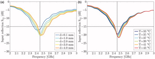
The sensitivity of the reflected power of the antenna, i.e. S₁₁ is shown in Figure 3(a) as function of frequency and for varying distance (d). It can be seen that the antenna input return loss is well below −15 dB for a bandwidth of nearly 100 MHz over the complete range of d. Simulations with feed lines positioned on the PCB surface displayed high power losses due to reflections at the air–water interface (results not shown), confirming that embedding the feed lines within the PCB indeed makes the antenna insensitive to the exact location of the air–water interface. Figure 3(b) shows the antenna reflection coefficient for a range of water temperatures. The results demonstrate that the applicator operates within requirements and is not very sensitive for water temperature variations.

Figure 3. (a) Reflection coefficient for various water levels as measured at a water temperature of 37 °C. (b) Reflection coefficient for various water temperatures at a distance (d) of 3.0 mm.

Experiment 1: Heating performance

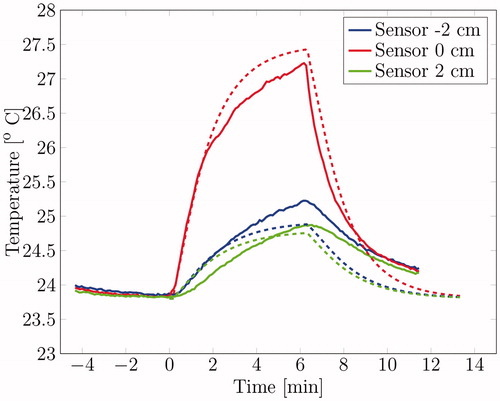
The temperature increase at various locations along the centre axis within the phantom were monitored (see Figure 2 for the sensor locations). Figure 4 depicts the measured (solid lines) and simulated (dashed lines) temperature profile over time at different locations along the major axis of the cylindrical muscle equivalent phantom. During the heating, the simulated temperature differed max. 0.53 °C for the red line, 0.20 °C for the blue line and 0.22 °C for the green line. The simulation tends to overestimate the temperature increase for the probe close to the antenna (sensor 0 cm). The initial temperature rise per second for the red line is 0.026 °C/s when the heating starts, resulting in a SAR of 94.6 W/kg when assuming a thermal capacity of 3640 W/kg/°C. The SAR as predicted by our simulation was 95.3 W/kg, so the difference between predicted and measured power-uptake was only 0.7%. The temperature decrease when the power is shut down is slightly higher, 0.031 °C/s.

Figure 4. The temperature profiles as generated from heating a cylindrical phantom with 16.5 W effective power at three locations: the middle and 2 cm shifted in each direction along the longitudinal axis. Measured (solid lines) and simulated (dashed lines) time–temperature profiles.

Experiment 2: Hot spot intensity and shape

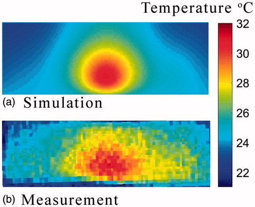
During Experiment 2, the temperature distribution of a sliced phantom after heating for 5 min with an effective power of 16.5 W was monitored using an IR-camera. Figure 5 shows the simulated and measured 2D heating pattern along the sagittal central plane of the cylindrical phantom. Overall, both graphs display similar trends regarding the temperature and size of the hot spot, and show a small asymmetry in the temperature distribution.

Figure 5. Simulated (a) and measured (b) temperature distributions (°C) for Experiment 2 (phantom length 80 mm, diameter 20 mm).

Experiment 3: MR-compatibility

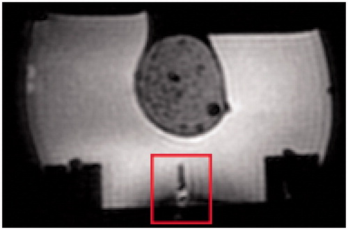
A typical MR scan is shown in Figure 6. Some minor distortions can be seen around the antenna, but no disturbances are visible in the area of interest, i.e. the phantom (circular shape above the antenna).

Figure 6. Magnitude scan of the applicator. The antenna is located in the red square at the lower centre region.

Simulation with mouse model

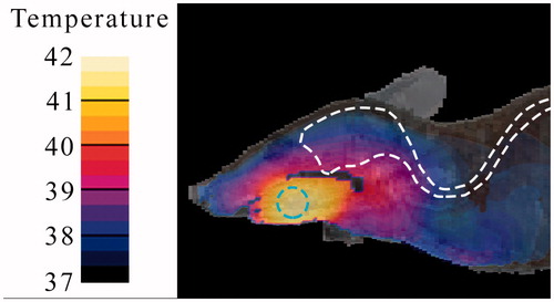
The simulated temperature distribution at the base of the tongue in the mouse anatomy during heating with the applicator is shown in Figure 7. The simulated temperature in the target area ranges from 41.0 to 41.7 °C while the brain temperature increases by ∼1° with a small area being heated by 2°.

Figure 7. A cutout of the temperature distribution in Celcius degrees as generated by the antenna radiating at 20 W. The boundary of the sensitive tissues is marked by the white dashed line and the target area with cyan.

Discussion

The antenna performance tests demonstrate that the antenna input return loss does not change significantly for realistic changes in the antenna environment (water level and temperature). This confirms that embedded feed lines stabilise the antenna matching; that its position within the scaffold will not have a big influence on the SAR distribution generated; and that the applicator can be used under various circumstances.

The simulated temperature distribution as calculated for the configuration in the first experimental set-up show a good agreement with the measured temperature in the first heating experiment (see Figure 4). The SAR as simulated is in good agreement with the SAR as calculated from the specific heat capacity and initial temperature rise for two of the three sensors. The sensor at 2 cm does not agree with the simulation, probably due to a deviation in its positioning or the presence of an air bubble or local phantom material inhomogeneity.

Note that the temperature decrease per second of the middle sensor is slightly higher than the initial temperature rise, while they should in theory be equal. This theory does not apply in this situation; however, since the steady state was not reached when the source was turned off. Next to that, the power source does not generate the same amount of power over time, so the SAR distribution might have varied. The temperature decrease per second of both other sensors deviate too, but this can easily be explained. Since they are not positioned near the hot spot, they receive energy from the antenna as well as from hotter regions trough heat conduction.

The temperature increase in the middle sensor (at 0 cm) deviates from the simulated temperature. This could be due to inhomogeneous cooling effects. The convective heat transfer rate of water increase with the Reynolds number (a measure for the turbulence of the water flow) [26]. This Reynolds number is higher when the water flow is obstructed, thus at the site of the antenna. Next to that, the water flow could vary within the water bolus, which has an irregular shape. Because of these effects, the water cooling near the middle sensor is probably different from other sites, while they are modelled with the same convective heat transfer rate. Other explanations for the deviation in temperature are positioning errors of the temperature sensors, which are significant close to the hot spot, and local inhomogeneities, which effect material parameters like the permittivity, conductivity and thermal conductivity.

The results of the second experiment agree with the trends depicted by the related simulation (see Figure 5). The size, location and temperature of the hot spot and the small asymmetry match.

In both experiments, minor spatial differences between the model and the experimental setup can cause significant changes in the outcome of an experiment. The positioning of the antenna, phantom and temperature probe are done by hand while working on a millimetre scale. Hence, measures need to be included for accurate positioning. Earlier, we already reported the need to improve on positioning accuracy with increasing frequency when we reported the translation of HT treatment modelling during HT of H&N tumours using the Hypercollar3D [32]. This means that a sensitivity analysis is of great importance when further researching the possibilities of heating with the applicator.

The MR measurements show that the HT device is able to operate within an MR-scanner without causing much disturbance. However, a qualitative analysis of the setup needs to be conducted still. The temperature increase reached in an MR-environment should be validated, as well as the accuracy of the temperature measurement.

The simulations regarding the mouse model show a temperature distribution fulfilling the requirements for the applicator, using electromagnetic waves to increase the temperature locally to at least 41 °C. The modelling illustrates the potential of the applicator for heating anthropomorphic H&N tumours. Clearly, the present result is an estimate of the heating pattern and not of the absolute temperature, since our mouse model is not complete. The cooling properties of a water bolus in mice could be different and global thermoregulation has been ignored. Note that the much higher surface area-to-body ratio (SA/V) in rodents makes global thermoregulation much more prominent. Furthermore, perfusion data largely based on large animals was used in absence of mouse-related data. Different blood perfusion-related heat conduction would lead to a change in focus size and perfusion values difference would lead to a different steady state temperature. Nevertheless, we expect that our results provide an adequate estimation of the in vivo focus spot location and of the relative temperatures that this setup generates in target and normal tissues. Hence, the theoretical analysis shows that our HT device is able to create a local hot spot of 41 °C, but in vivo experiments are necessary to validate the actual device performance.

Conclusions

This study outlines the design and working conditions of a H&N small-animal HT applicator based on a 2.45 GHz resonant PCB antenna embedded in a water bolus. A satisfactory agreement between simulated and measured temperature distribution values was reached and it was experimentally demonstrated that a focussed hot spot can be created with the described system. An MR-experiment was conducted to show that the setup is able to operate within an MR-environment, which is essential for precise 3D thermal dosimetry. Lastly, a simulation including a virtual mouse was used to show that the system is able to create a local hot spot of 41 °C in the area of interest, the tongue area.

In further research, we plan to quantitatively validate the temperature rise and MR thermometry in different in vivo heating scenarios.

Acknowledgements

The authors like to thank Tomas Drizdal for sharing his advice and expertise for the development of the HT applicator. Special thanks go to Ali Ameziane, Joost Haeck and Daniël de Jong for their help with the experiments.

Disclosure statement

The authors report no declarations of interest.

Notes

Additional information

Funding

This work has been made possible with KWF Kankerbestrijding (Dutch Cancer Society; project no. EMCR-2012–5472).

Notes

1 SEMCAD X v. 14.8, SPEAG, Zurich, Switzerland.

2 Sim4Life v. 3.2.2, SPEAG, Zurich, Switzerland.

References

- Eppink B, Krawczyk P, Stap M, Kanaar JR. (2012). Hyperthermia-induced DNA repair deficiency suggests novel therapeutic anti-cancer strategies. Int J Hyperthermia 28:509–17.
- Jansen W, Haveman J. (1983). Histopathological changes in the skin and subcutaneous tissues of mouse legs after treatment with hyperthermia. Pathol Res Practice 186:247–53.
- Sano D, Myers JN. (2009). Xenograft models of head and neck cancers. Head Neck Oncol 1:32.
- Salahi S, Maccarini PF, Rodrigues DB, et al. (2012). Miniature microwave applicator for murine bladder hyperthermia studies. Int J Hyperthermia 28:456–65.
- Terentyuk GS, Maslyakova GN, Suleymanova LV, et al. (2009). Laser-induced tissue hyperthermia mediated by gold nanoparticles: toward cancer phototherapy. J Biomed Optics 14:021016.
- Adela B, Mestrom RMC, Paulides MM, Smolders AB. An MR-compatible printed Yagi-Uda antenna for a phased array hyperthemia applicator. Proceedings of the 7th European Conference on Antennas and Propagation (EUCAP); 2013; Gothenborg, Sweden.
- Hasgall PA, Di Gennaro F, Baumgartner C, et al. (2015). IT'IS database for thermal and electromagnetic parameters of biological tissues, Version 3.0. doi: 10.13099/VIP21000-03-0
- Koledintseva MY, Pommerenke DJ, Drewniak JL. FDTD analysis of printed circuit boards containing wideband Lorentzian dielectric dispersive media. 2002 IEEE International Symposium on Electromagnetic Compatibility; 2002; Minneapolis.
- Stogryn AP. (1971). Equations for calculating the dielectric constant of saline water. IEEE Trans Microw Theory Tech 19:733–6.
- Ito K, Furuya K, Okano Y, Hamada L. (2001). Development and characteristics of a biological tissue-equivalent phantom for microwaves. Electron Comm Jpn 84:67–77.
- Ramette JJ, Ramette RW. (2011). Siphonic concepts examined: a carbon dioxide gas siphon and siphons in vacuum. Phys Educ 46:412–16.
- Society for Thermal Medicine. (2016). ICHO Award Winners. Available from: http://www.thermaltherapy.org/ebusSFTM/ANNUALMEETING/2016ICHOMEETING/AwardWinners.aspx [last accessed 1 Sep 2016].
- Müller J, Hartmann J, Bert C. (2016). Infrared camera based thermometry for quality assurance of superficial hyperthermia applicators. Phys Med Biol 61:2646–64.
- de Bruijne M, Samaras T, (2006). Effects of waterbolus size, shape and configuration on the SAR distribution pattern of the Lucite cone applicator. Int J Hyperthermia 22:15–28.
- Christie IS, Patel JR, Toledo RT. (2005). Fluid to particle heat transfer coefficients in holding tube having noncircular cross section. J Food Sci 70:338–43.
- PaulidesStauffer M, Neufeld PE, MacCarini P, et al. (2014). Simulation techniques in hyperthermia treatment planning. Int J Hyperthermia 29:346–57.
- Song C. (1984). Effect of local hyperthermia on blood flow and microenvironment: a review. Cancer Res 44:4721–30.
- Verhaart RF, Verduijn G, Fortunati M, et al. (2015). Accurate 3D temperature dosimetry during hyperthermia therapy by combining invasive measurements and patient-specific simulations. Int J Hyperthermia 31:686–92.
- Togni P, Rijnen Z, Numan WCM, et al. (2013). Electromagnetic redesign of the HYPERcollar applicator: toward improved deep local head and-neck hyperthermia. Phys Med Biol 58:5997–6009.
- Colombo R, Salonia A, Leib Z, et al. (2010). Long-term outcomes of a randomized controlled trial comparing thermochemotherapy with mitomycin-C alone as adjuvant treatment for non-muscle-invasive bladder cancer (NMIBC). BJU Int 107:912–18.
- Datta N, Puric R, Heüberger E, et al. (2015). Hyperthermia and reirradiation for locoregional recurrences in preirradiated breast cancers: a single institutional experience. Swiss Med Wkly 145:w14133.
- Issels R, Kampmann E, Kanaar R, Lindner LH. (2016). Hallmarks of hyperthermia in driving the future of clinical hyperthermia as targeted therapy: translation into clinical application. Int J Hyperthermia 32:89–95.
- Paulides MM, Verduijn GM, Holthe NV. (2016). Status quo and directions in deep head and neck hyperthermia. Radiat Oncol 11:21.
- Hijnen NM, Heijman E, Köhler MO, et al. (2012). Tumour hyperthermia and ablation in rats using a clinical MR-HIFU system equipped with a dedicated small animal set-up. Int J Hyperthermia 28:141–55.
- Paulides MM, Bakker JF, Chavannes N, Rhoon GCV. (2007). A patch antenna design for application in a phased-array head and neck hyperthermia applicator. IEEE Trans Biomed Eng 54:2057–63.
- Singh AK, Moros EG, Novak P, et al. (2004). MicroPET-compatible, small animal hyperthermia ultrasound system (SAHUS) for sustainable, collimated and controlled hyperthermia of subcutaneously implanted tumours. Int J Hyperthermia 20:32–44.
- Dunwiddie TV, Worth T. (1982). Sedative and anticonvulsant effects of adenosine analogs in mouse and rat. J Pharmacol Exp Ther 220:70–6.
- IT’IS (The Foundation for Research on Information Technologies in Society). (2012). Female OF1 mouse V1.0. IT’IS Foundation, Zurich, Switzerland. DOI: 10.13099/VIP91203-01-0. [Online]. Available from: https://www.itis.ethz.ch/virtual-population/animal-models/animals/female-of1-mouse-3/female-of1-mouse-v1-0/ [last accessed July 2014].
- Lessin AW, Parkes MW. (1957). The relation between sedation and body temperature in the mouse. Br J Pharm Chemother 12:245–50.
- Paulides MM, Mestrom RMC, Salim G, et al. (2017). A printed Yagi–Uda antenna for application in magnetic resonance thermometry guided microwave hyperthermia applicators. Phys Med Biol 62:1831–47.
- Dillon CR, Vyas U, Payne A, et al. (2012). An analytical solution for improved HIFU SAR estimation. Phys Med Biol 57:4527–44.
- Roemer RB, Fletcher AM, Cetas TC. (1985). Obtaining local SAR and blood perfusion data from temperature measurements: steady state and transient techniques compared. Int J Radiat Oncol Biol Phys 11:1539–50.