Real-time estimation of lesion depth and control of radiofrequency ablation within ex vivo animal tissues using a neural network

Abstract

Background: Radiofrequency ablation (RFA), a method of inducing thermal ablation (cell death), is often used to destroy tumours or potentially cancerous tissue. Current techniques for RFA estimation (electrical impedance tomography, Nakagami ultrasound, etc.) require long compute times (≥ 2 s) and measurement devices other than the RFA device. This study aims to determine if a neural network (NN) can estimate ablation lesion depth for control of bipolar RFA using complex electrical impedance – since tissue electrical conductivity varies as a function of tissue temperature – in real time using only the RFA therapy device’s electrodes.

Methods: Three-dimensional, cubic models comprised of beef liver, pork loin or pork belly represented target tissue. Temperature and complex electrical impedance from 72 data generation ablations in pork loin and belly were used for training the NN (403 s on Xeon processor). NN inputs were inquiry depth, starting complex impedance and current complex impedance. Training-validation-test splits were 70%-0%-30% and 80%-10%-10% (overfit test). Once the NN-estimated lesion depth for a margin reached the target lesion depth, RFA was stopped for that margin of tissue.

Results: The NN trained to 93% accuracy and an NN-integrated control ablated tissue to within 1.0 mm of the target lesion depth on average. Full 15-mm depth maps were calculated in 0.2 s on a single-core ARMv7 processor.

Conclusions: The results show that a NN could make lesion depth estimations in real-time using less in situ devices than current techniques. With the NN-based technique, physicians could deliver quicker and more precise ablation therapy.

Keywords:

• Ablation
• control
• radiofrequency
• neural
• machine
• learning
• depth

Introduction

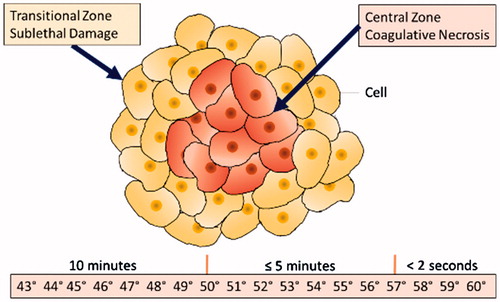
Radiofrequency ablation (RFA) is commonly used to destroy liver, kidney, lung and bone tumours and other potentially cancerous tissues. RFA heats tissue with electrodes that supply alternating electric current, which causes ionic agitation and joule heating [1–4]. When cells are exposed to the temperatures shown in Figure 1, they undergo coagulative necrosis (i.e. ablation). Additionally, DNA repair and metabolism are impaired in cells exposed to sublethal temperatures in the transition zone [1]. However, as the tissue in the depth-axis is not visible due to the opacity of tissue, it is difficult to visually monitor RFA progress in real time. Point temperature probes are included in many RFA devices, but do not provide three-dimensional lesion depths [1,2]. Feedback control requires monitoring of RFA lesion progress as tissue left unablated could locally recur (underablation); likewise, without knowledge of lesion depth, critical structures deeper within tissue could be damaged (overablation) [3–5].

Figure 1. Temperatures and times for thermal damage within tissue.

As of late 2017, there is quite a significant amount of work done by the scientific community to develop techniques for monitoring the progress of RFA treatment and lesion depths in real time. These techniques utilise changes in tissue properties undergoing thermal ablation, including electrical, acoustic and optical behaviours. Electrical impedance tomography uses surface electrodes surrounding the tissue under evaluation to measure impedance paths that are reconstructed into tissue electrical conductivity to provide lesion depth images that can be 90%+ accurate [4,6–8]. While data collection is quick, reconstruction is complex due to the requirement of solving the ill-posed three-dimensional inverse problem [6–8]. Thus, computing a single EIT-based lesion depth map requires time on the order of seconds (time increases with accuracy from ≥ 2 s for 70% accuracy to ≥ 100 s for 90%+ accuracy) and ≥ 1 gigabyte of memory on ×86 processor-based workstations, despite many strides in the speed of reconstruction algorithms [6–8]. Recently, Nakagami-based ultrasound imaging using conventional pulse-echo systems, instead of custom elastic strain systems, has been shown to provide 94% accuracy for monitoring RFA lesions in liver tissues in real-time (0.5–1.0 s compute time on ×86 workstations), but these systems cannot image muscular tissue [5]. Optoacoustic imaging, a combination of optical and acoustic techniques, uses pulses of lasers to excite tissue and ultrasonic sensor arrays to record acoustic emissions from these light pulses [9,10]. While optoacoustic methods are 95%+ accurate in the mm scale, construction of the three-dimensional lesion depth map from the data requires computation on the order of ≥ 400 s [9,10]. Despite the high accuracy and possibility of real-time data collection from these current RFA monitoring methods, it is not yet possible to compute lesion depth maps for all soft tissues in real-time using standard embedded system hardware.

In addition to the computational complexity of current techniques, there are clinical use pitfalls as well. For example, EIT electrodes (16 + placements usually) are cumbersome and time-consuming to place, requiring that physicians place electrodes exactly on a straight plane with good contact, as reconstructions are highly sensitive to placement and electrical noise [11,12]. One group improved EIT electrode placement techniques by developing a stretching electrode belt method for human torsos, but this still requires circumferential placement on patients, which may not be possible if the ablation site opening interferes with placement [13]. In addition, current acoustic imaging techniques require that physicians hold the imaging probe during ablation [5,10]. Thus, it is desirable to develop a monitoring technique that can utilise tissue properties without requiring additional external probes or additional clinical effort.

Artificial neural networks (ANN) have made significant strides in the late 2010s, most notably the real-time approximate computation of the Navier–Stokes fluid equations [14,15]. These works have shown that artificial neural networks are able to approximate the solutions to partial differential equations in real-time, speeding up computation time significantly by 2–4 orders of magnitude over finite element analysis techniques (similar to some EIT reconstruction algorithms) while retaining 90%+ accuracy [14,15]. Recent biomedical imaging or monitoring-related applications of ANNs are concentrated in biomedical image classification, where ANNs perform fast, automatic classification of images and cancer presence [16–18]. The main advantage of these ANN-based systems is faster, improved reporting from radiologists and pathologists on the presence of disease. However, ANN-based methods require diverse training data to fully learn relationships and are susceptible to poor choices of feature descriptors (parameters input into the ANN); nevertheless, when feature descriptors are chosen well, ANNs are highly accurate [16–18]. For example, a skin cancer imaging segmentation and classification ANN performed as well as or better than dermatologists against a known training set [17]. As with all ANNs, the training set needed for such high accuracy must be large, so the skin cancer study used 1.41 million training images [17]. Thus, the trade-off with ANNs is between fast, accurate real-time computation performance and large, accurate training data sets.

From these recent advances in ANNs, our group hypothesised a feed-forward ANN might be able to compute in real-time the lesion depth from RFA within biological tissue with 80%+ accuracy. The hypothesised ANN would not require significant additional probes or equipment besides the RFA device. As far as we are aware, this is the first time that an ANN has been applied for RFA monitoring and/or control. Keywords used for searching included: “ablation”, “radiofrequency”, “machine”, “learning”, “neural” and “network”, within databases including Google Scholar, PubMed and IEEE Xplore.

In this study, an ANN was used as a depth estimation system that approximates the lesion depth map solution of a pseudo-EIT system based on the Laplace and joule heating equations. The depth estimation system we developed enables fast computation with embedded microprocessors since neural networks are non-linear weighted sums. Our depth estimation maps computed in under 0.2s on embedded microprocessors. Data are collected using only the multipolar RFA device electrodes. The neural network-based depth estimator utilises the same temperature-based and cellular morphology-based tissue electrical property changes employed in EIT systems for RFA, primarily utilising changes in electrical conductivity and complex electrical impedance. In this study, we present an experimental proof-of-concept study within ex vivo animal tissues of the utilisation of an ANN for monitoring and control of RFA therapy. The study is split into two parts: (1) collecting data for training via ablation within target tissues followed by training/testing of the ANN as a lesion depth estimator and (2) application testing of the depth estimator when used as part of a feedback-based automatic ablation control system within tissue to target lesion depths.

Materials and methods

Tissue model

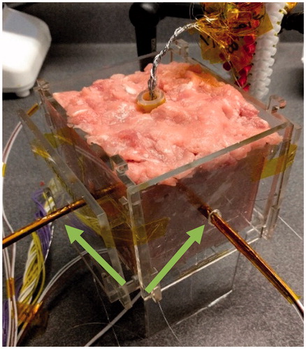
Tissue models used for training and testing the neural network consisted of fresh-ground pork loin and pork belly and beef liver (only used for testing). Gross analysis was used to measure the ablation lesion depths, as the discoloured gross lesion margin closely correlates with microscopic histopathological staining necrosis margins in muscle and liver tissues [19–21]. Samples were heated to near-physiological temperature (34 °C) and placed into the centre of an 80-mm × 80-mm × 80-mm acrylic fixture (Figure 2). The 40-mm diameter RFA device used was placed directly into the centre of the fixture, maintaining 20-mm of tissue clearance between the centre of each panel of the acrylic fixture and the closest side of the RFA device. The initial tissue electrical conductivities were not computed, as is standard in EIT, since the initial complex impedance magnitude parameter is the weighted sum of electrical resistivity (reciprocal of electrical conductivity) of tissues and thus defines starting tissue conditions indirectly within the neural network.

Figure 2. Tissue fixture for ablation data collection. Green arrows indicate the temperature probes, which are inserted into the tissue model perpendicular to each face.

Measurement/ablation hardware configuration

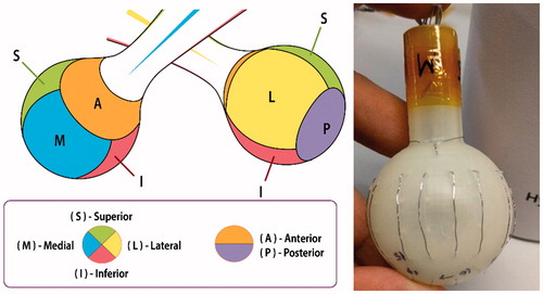
The RFA device (Figure 3) used during the training and testing studies was a multipolar design, with each exposed stainless steel 316 electrode (AM Systems, Carlsborg, WA) individually connected to a matrix switch (National Instruments PXIe-2529, Austin, TX). The geometry of the device is spherical, with six active faces, each corresponding to a clinical margin. For simplicity and speed of data collection, the four electrodes of each device face were grouped together as one connection by the matrix switch, thus presenting a measurement of the entirety of each device face.

Figure 3. RFA device design with six faces, each corresponding to a clinical margin (left). Prototype with 4 electrodes per face and ring electrode at anterior face (right).

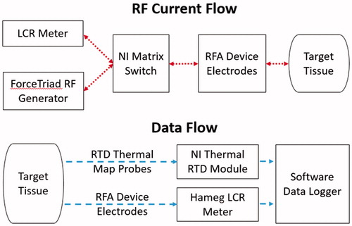
The matrix switch was also connected to a LCR (inductance, capacitance, resistance) meter (Hameg HM8118, Columbia, MD) and RF power generator (Covidien ForceTriad, Boulder, CO) set to 30 W output (Figure 4). The LCR meter was the measurement device for the complex electrical impedance data and thus also potentially introduced measurement noise or error within the data collected. All complex electrical impedance data were collected at a single spot frequency of 100 kHz, within the RF ablation frequency range, rather than multiple spot frequencies. At 100 kHz, the measurement error of the LCR meter used for collecting complex electrical impedance data was within about 0.5% of the true value, according to the user manual. To improve the certainty of the collected data and remove erroneous measurements, a truncated mean using six samples was used for each impedance measurement. The single spot frequency strategy was chosen for quicker prototyping and proof of concept since measurements at additional frequencies would only increase the accuracy of the system. This is due to the properties of ablated tissue, which after having undergone coagulation, will not vary as significantly in electrical conductivity across different frequencies under 1 MHz [4].

Figure 4. RF current flow and dataflow architecture of depth estimator training system.

A resistance temperature detector (RTD) signal conditioning input module (National Instruments PXIe-4357, Austin, TX) recorded temperature data from temperature probes at 2 Hz fabricated using carbon fibre tubes (Rock West Composites, San Diego, CA) and platinum 100-ohm resistance temperature detectors (RDF Corp, Hudson, NH) spaced at 5 mm interval depths from the tip of the carbon fibre tube. Thus, each temperature probe consists of RTDs measuring 0, 5, 10 and 15 mm depths from each device face. A ×86–64 Xeon (Intel, Santa Clara, CA) microprocessor-based workstation was used for operating the matrix switch, logging data and optimising and training the depth estimation neural network. A development board with a ARMv7 embedded microprocessor (BCM2836, Broadcom, Irvine, CA) with 512MB of memory was employed for testing the computation time and memory usage of a full depth estimation map.

Depth estimator software architecture

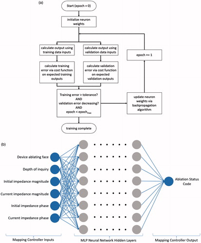
The depth estimator is a multilayer perceptron (MLP), a type of feed-forward artificial deep neural network from the scikit-learn Python library (INRIA, Rocquencourt, France). The MLP depth estimator is a directed network configured with four hidden layers and 60 nodes in each layer, resulting in 14 400 weights to tune (Figure 5). The estimator, when trained, will yield a computation of a non-linear function on the weighted input sum at each neuron. Thus, if a neuron i in layer n has input weights w and input values v from the previous neuron j, and the non-linear activation function is g, then the output value y of the neuron is: (1)

Figure 5. (a) Backpropagation-based multilayer perceptron training algorithm flowchart. (b) Architecture of the multilayer perceptron used for depth estimation.

Our MLP depth estimator used the rectified linear unit function g for the non-linear activation function on each hidden-layer neuron: (2)

Other activation functions, such as the logistic sigmoid or hyperbolic tangent functions, will yield different results. The output layer makes the final transformation of the output values of the last hidden layer to a binary classification. The output layer activation function is the logistic sigmoid (3), which makes the cost function differentiable for gradient descent solvers. (3)

Training occurred via a backpropagation-based algorithm (Figure 5(b)) which utilised the logarithmic binary cross-entropy (4) as the cost function on the output layer and the ADAM stochastic solver [22–24]. The logarithmic binary cross-entropy function is as follows, where n is the number of instances of training data, x is the set of training data, y is the set of expected outputs and a is the neural network function and returns the neural network output: (4)

The weights of the network were initialised by using a zero-mean uniform distribution in the range which provides extremely stable training results [25,26].

Six features (parameters) were input into the neural network as floating-point numbers: device ablating face, depth of inquiry (measurement position), initial impedance magnitude, current impedance magnitude, initial impedance phase and current impedance phase.

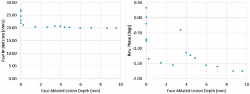
The output was a binary classification of whether the tissue volume at the face and depth specified was ablated or not (ablation status code). Temperature data were used to calculate the output labels for training, where tissues at 43 °C  for ≥10 min, 50 °C + for ≥5 min and 57 °C + for ≥2 s were considered ablated. The ablation heating times and temperatures were chosen from literature of cell death exposure models used in RFA studies [1–4]. A cell that reaches 57 °C undergoes near-instantaneous coagulation and necrosis; similarly, when cells are exposed to high temperatures for extended periods of times (43 °C for >10 min, 50 °C for >5 min), the cells undergo protein coagulation, causing coagulative necrosis [1,2]. Sample data of the ablation lesion depth of the margin in millimetres are plotted against complex electrical impedance for one face in Figure 6. The data in Figure 6 show that there are general trends for the complex electrical impedance as the ablation lesion of a particular face grows deeper. Thus, suggesting the ANN can model the trends with respect to the tissue ablation status.

Figure 6. Sample depth-based impedance magnitude and phase training data.

Ablation controller software architecture

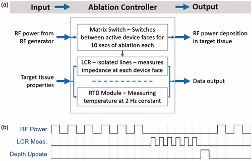
A software component with real-time execution was created to automate switching and data collection with the hardware system. The ablation controller software operates the LCR meter, matrix switch and RTD module (Figure 7(a)). To prevent interference between the LCR meter and the RF generator, the RF generator and LCR meter lines were mutually exclusive on the switch and on/off periods were alternated (Figure 7(b)). After all enabled device faces delivered power to their local tissue for 10 s each, the ablation controller software collected complex electrical impedance for all device faces. Temperature was collected during all times at 2 Hz, with interpolated temperatures in between 0.5 s measurement intervals.

Figure 7. (a) Ablation controller software architecture flowchart. (b) Timing diagram of how ablation, measurement, and computation occur.

Study Part 1: depth estimator training

To generate the data needed for training, experiments were performed with the hardware within the tissue models described. For each training data generation ablation, one face (tissue margin) was ablated to further depths than the other five faces. For example, the further-ablated face (manual target of 15 mm) may have had 50 total ablation-measurement cycles, while the shorter-ablated faces (manual target of 10 mm) may have had 50 total measurement cycles and only 35 ablation cycles. Thus, the ablation shape of the data collected is similar to an ellipsoid. Each training ablation produced up to 300 samples of input data from the number of complex electrical impedance measurements per ablation run. In turn, since each time point has different ablation depths, the ablation depth per time point was calculated using the temperature point at that time point, according to the previously described calculation in the Software Architecture section. Since each face has 151 estimation depth points (due to the 0.1 mm stepping from 0.0 mm to 15.0 mm), a sample training ablation can generate up to 46 000 data points. In total, 72 data generation ablations (36 pork loin and 36 pork belly) were performed, resulting in 1 872 000 total data points for the training-validation-testing data set. Two data set split sets were compared for training-validation-testing of the MLP classifier, 80%-10%-10% and 70%-0%-30%. The data within each split were randomly selected from the overall data set.

Study Part 2: depth estimator-controlled RFA application testing

The trained MLP neural network was then integrated into a depth estimator software component to test the application performance of the neural network as part of an automatic feedback control system for RFA. The depth estimator software receives complex electrical impedance data, computes lesion depth estimations using the trained MLP neural network and replies with lesion depth estimated data. This interfaced with the ablation controller software, which then operated automatically due to this new closed feedback loop. To receive a lesion depth estimation, the ablation controller software sends a request containing the measured impedance data to the depth estimator. The requests from the ablation controller software contain the data values for the features, and the real-time responses from the depth estimator software provide depth estimations for the ablation controller software. The ablation controller software will disable a device face from being connected to the RF generator on the switch upon the target lesion depth per face being reached according to the depth estimation software response.

This automated ablation control software was tested not only within the trained tissues (pork loin and pork belly), but also within an untrained tissue, beef liver, to test the extrapolation potential of the MLP classifier for decisions within tissues not present within the training data set. This extrapolation potential is important because of the limited number of in vivo or ex vivo human tissue samples that can be acquired in comparison to more-available animal tissue samples. Another important aspect was the high plurality of liver as a test tissue model for RF ablation [1–5]. For all tissue tests, except for two tests, the automatic target lesion depth was set to 5 mm for all sides except for one side at 10 mm. For the two exceptions, the automatic target lesion depth was set to 10 mm for all sides except for one side at 15 mm to explore the performance at deeper ablation depths.

Results

Study Part 1: depth estimator training results

The training computation for the MLP classifier finished in 403 s on an ×86–64 microprocessor-based workstation (Supermicro, San Jose, CA) with 16GB of memory. Export of the trained neural network weights to C language-based weighted sum execution code compiled for the ARMv7 embedded microprocessor showed that computation of a full depth estimation map could occur within 0.20 s. Using the same C language-based code compiled for the ×86–64 workstation microprocessor, the depth estimation map was computed within 0.02 s.

The multilayer perceptron (MLP) classified tissue ablation status quite well using only features related to complex electrical impedance at 100 kHz. Table 1 shows the confusion matrix output statistics for the MLP classifier with a training-validation-testing data set split of 80%-10%-10%, while Table 2 shows the confusion matrix output statistics for the MLP classifier with a training-validation-testing data set split of 70%-0%-30%. The confusion matrix in both tables are calculated where true negatives are depths reported by the depth estimator to be unablated and truly unablated, and true positives are depths reported by the depth estimator to be ablated and truly ablated. The MLP classifies tissue ablation status with a spatial resolution of 0.1 mm, for all depths up to 15 mm, the maximum depth trained with the classifier. Minimal differences were observed when using the training-validation-testing data set split of 70%-0%-30% versus a training-validation-testing data set split of 80%-10%-10%, indicating a sufficient number of training data points. Overfitting was not an issue as shown in the convergence curve in Figure 8, where training and validation curves do not deviate in slope sign. The accuracy, overprediction (false positives) and underpredictions (false negatives) are plotted by ablation depth on Figure 9. This was generated by comparing the classifier output label against the expected output label.

Figure 8. Training convergence plot for 80-10-10 training-validation-test split.

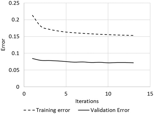
Figure 9. Final trained accuracy of MLP classifier as used for control system.

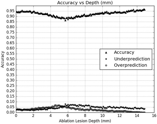
Table 1. Output statistics for multilayer perceptron when trained using 80%-10%-10% train-validate-test data set split. Statistics are based on using the 10% testing data split.

	80-10-10 split (train n = 1 497 600; validate n = 187 200; test n = 187 200)
Accuracy	93%
Precision	85%
True positive rate	91%
False positive rate	6%

Table 2. Output statistics for multilayer perceptron when trained using 70%-0%-30% train-validate-test data set split. Statistics are based on using the 30% testing data split.

	70-0-30 split (train n = 1 310 400; validate n = 0; test n = 561 600
Accuracy	93%
Precision	90%
True positive rate	87%
False positive rate	4%

Study Part 2: depth estimator-controlled RFA application test results

The test results for the depth estimator-controlled RFA tests are presented in Table 3. The difference is calculated as target lesion depth minus actual lesion depth, where the actual lesion depths are measured as whole integer millimetres via macroscopic analysis of colour change present within tissue upon thermal ablation due to protein coagulation [1–3]. Table 4 breaks down the data in Table 3 by the target lesion depth. The technique of sectioning is presented in Figure 10. A representative test result, Figure 11, shows that, for a target lesion depth of 5 mm for all sides except two 10 mm sides, the neural network-based depth estimator-controlled RFA system produced the target lesion geometries. An additional tissue type not trained within the classifier but still tested was bovine liver given its common use within RFA experiments. The bovine liver tests produced the least difference, but also have fewer samples than the pork types. Overall, the system overall ablated the tested tissue types to a mean difference of −0.7 mm.

Figure 10. Illustration of how tissue is sectioned for macroscopic analysis.

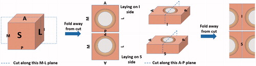
Figure 11. Ablation sample showing the desired deeper lesion depth in two device faces and uniform lesion depths in four other device faces. Scale legends are on images.

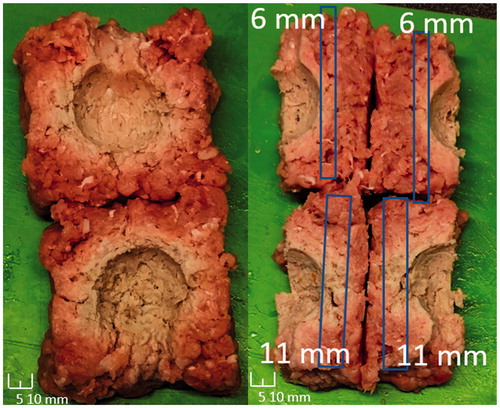
Table 3. Overall depth estimator-based control testing results, where the difference is between the target ablation depth and the system-controlled ablation depth.

Tissue model	Sample measured	Mean difference (mm)	Standard error (mm)
Ground pork loin	40	−1.2	0.4
Ground pork belly	40	−0.5	0.3
Whole beef liver	30	−0.1	0.4
All tissue types	110	−0.7	0.2

Table 4. Overall depth estimator-based control testing results by target depth, where the difference is between the target ablation depth and the system-controlled ablation depth.

Tissue model	Target depth (mm)	Samples measured	Mean difference (mm)	Standard error (mm)
Ground pork loin	5	18	−3.2	0.4
	10	18	0.3	0.4
	15	4	1.0	0.4
Ground pork belly	5	24	−1.0	0.2
	10	16	1.9	0.5
Whole beef liver	5	18	−1.9	0.3
	10	12	0.4	0.4

Discussion

Neural network depth estimation discussion

As the results show, a deep neural network can learn the relationship between electrical impedance/conductivity and ablation status within biological tissues. The neural network trained to 90%+ accuracy (Tables 1 and 2) without requiring external electrodes or significant additional equipment external to the target tissue sample, significantly reducing the amount of hardware required to actively control a RF ablation procedure. However, as mentioned in the introduction, all machine learning classifiers require a large and consistent training data set for high accuracy [16–18]. The final system had underestimation errors (Figure 9) that could be corrected or reduced significantly by training with a larger, more diverse data set.

The performance of the depth estimator within untrained beef liver in Tables 3 and 4 (overablation of 1.9 mm at 5 mm and underablation of 0.4 mm at 10 mm) show that the quantity and limited diversity of training data within this proof-of-concept system seemed to be potentially sufficient for other homogeneous tissues with similar electrical and thermal properties than the training tissues. As described in the methods, training data were collected from only pork loin and pork belly, and the bovine liver tests were conducted without first training the neural network with beef liver training ablations. The performance of our system within this newly encountered tissue model demonstrates some potential of extrapolation with neural network-based depth estimation. We do expect, though, that extending the system for in vivo use requires additional training tissue models that include fatty, lean or vessel-heavy tissues at each face as well as within ex vivo human samples.

Another issue is the design of the neural network itself, which was a four-layer multilayer perceptron with rectified linear activation functions within this study. This simpler structure was chosen for quick proof-of-concept, since it would represent the worst-case architecture. A more tailored architecture, such as adjusting the activation functions, biasing certain features or using feedback loops, could potentially improve the accuracy and precision of the depth estimation [21–23,27–29]. The baseline architecture used worked quite well with the data as shown by the training and test results presented in the Results section, but these improvements should be further explored in future works.

Ablation system application discussion

Regarding potential improvements to the tissue measurement system, multiple spot frequency measurements may also increase the spatial resolution and accuracy of the system, as described in the methods. Increased spatial resolution could potentially allow for classification closer to the ground truth, as the feature set increases by an additional decimal digit (hundredths of millimetres, instead of just tenths of millimetres). Additionally, the developed system only measures current and voltage between two device faces (all four electrodes on one device face grouped), but a more complete tissue measurement system could drive current between two electrodes (or device faces) and measure the voltages present at the other electrodes or faces, providing the neural network with more parameters.

Timing of measurement cycles after ablation cycles is another potential issue. The current system scans the device face impedances in sequential order, with a single device face active on positive polarity and the other device faces active on negative polarity at any given scan. However, this imposes a sequentiality on the scan and ablation order. If a device face was not active during the previous ablation cycle, it may have different measurements than a device face that was active during the previous ablation cycle, simply due to the temperature of the tissue directly touching the electrode. Additionally, the system performs all ablation activations for an ablation cycle, then follows up with performing all measurement activations for a measurement cycle. This additional form of sequentiality means that tissue relaxation times (cool-down periods) between device face ablation activation and device face tissue measurement are not close or equal. Thus, the timing of the cycles is an additional limiting factor that could cause potential problems with heterogeneous tissues. These timing problems could potentially be remedied via the ablation controller software, either by face randomisation or face-by-face ablate-measure cycles.

Conclusions

These results of this study show the successful ability of a neural network to estimate ablation lesion depth in real-time without the need for significant additional equipment. Current technologies used for lesion depth estimation are generally limited by real-time computational demands and additional hardware in meeting clinical use requirements. The neural network-based system solves both computational and hardware challenges without significantly sacrificing accuracy or precision of ablation results. With this neural network-based depth estimation technique, physicians could potentially deliver quicker and more precise ablation therapy due to the real-time subsecond depth estimation map computation times and lack of external electrode placement. Future works will explore modifying the measurement frequency and timing, and optimising the neural network, to further improve results closer to the ground truth.

Acknowledgements

The authors would like to thank Michelle Hasse for her help with figures and insights into the tissue environments and considerations for technology applications.

Disclosure statement

In accordance with Taylor & Francis policy and ethical obligation as researchers, we are reporting that Y.C. Wang and T.C. Chan have financial interests in Innoblative Designs, Inc. that may be affected by the research reported in the enclosed paper. These interests have been disclosed fully to Taylor & Francis, and an approved plan for managing any potential conflicts arising from this arrangement is in place.

Additional information

Funding

This work was supported by the National Science Foundation under Grant ENG/IIP-1622842.

References

- Chu KF, Dupuy DE. (2014). Thermal ablation of tumours: biological mechanisms and advances in therapy. Nat Rev Cancer 14:199–208.
- Goldberg SN, Gazelle GS, Dawson SL, et al. (1995). Tissue ablation with radiofrequency: effect of probe size, gauge, duration, and temperature on lesion volume. Acad Radiol 2:399–404.
- Larina IV, Larin KV, Esenaliev RO. (2005). Real-time optoacoustic monitoring of temperature in tissues. J Phys D Appl Phys 38:2633.
- Wi H, McEwan AL, Lam V, et al. (2015). Real‐time conductivity imaging of temperature and tissue property changes during radiofrequency ablation: an ex vivo model using weighted frequency difference. Bioelectromagnetics 36:277–86.
- Zhou Z, Wu S, Wang CY, et al. (2015). Monitoring radiofrequency ablation using real-time ultrasound Nakagami imaging combined with frequency and temporal compounding techniques. PLoS One 10:e0118030.
- Cherepenin VA, Karpov AY, Korjenevsky AV, et al. (2002). Three-dimensional EIT imaging of breast tissues: system design and clinical testing. IEEE Trans Med Imaging 21:662–7.
- Javaherian A, Soleimani M, Moeller K. (2016). A fast time-difference inverse solver for 3D EIT with application to lung imaging. Med Biol Eng Comput 54:1243–55.
- Martin S, Choi CT. (2017). A post-processing method for three-dimensional electrical impedance tomography. Sci Rep 7:7212.
- Dean-Ben XL, Buehler A, Ntziachristos V, Razansky D. (2012). Accurate model-based reconstruction algorithm for three-dimensional optoacoustic tomography. IEEE Trans Med Imaging 31:1922–8.
- Pang GA, Bay E, Dean-Ben X, Razansky D. (2015). Three‐dimensional optoacoustic monitoring of lesion formation in real time during radiofrequency catheter ablation. J Cardiovasc Electrophysiol 26:339–45.
- Adler A. (2004). Accounting for erroneous electrode data in electrical impedance tomography. Physiol Meas 25:227.
- Graham BM, Adler A. (2007). Electrode placement configurations for 3D EIT. Physiol Meas 28:S29.
- Oh TI, Kim TE, Yoon S, et al. (2012). Flexible electrode belt for EIT using nanofiber web dry electrodes. Physiol Meas 33:1603.
- Tompson J, Schlachter K, Sprechmann P, Perlin K. (2016). Accelerating Eulerian fluid simulation with convolutional networks. Proceedings of the 34th International Conference on Machine Learning; Pre-print on 2016 Jul 13.
- Baymani M, Effati S, Niazmand H, Kerayechian A. (2015). Artificial neural network method for solving the Navier–Stokes equations. Neural Comput Appl 26:765–73.
- Cireşan DC, Giusti A, Gambardella LM, Schmidhuber J. (2013). Mitosis detection in breast cancer histology images with deep neural networks. International Conference on Medical Image Computing and Computer-assisted Intervention 2013 Sep 22 (pp. 411–18), Springer, Berlin, Heidelberg.
- Esteva A, Kuprel B, Novoa RA, et al. (2017). Dermatologist-level classification of skin cancer with deep neural networks. Nature 542:115–18.
- Li Q, Cai W, Wang X, Zhou Y, Feng DD, Chen M. (2014). Medical image classification with convolutional neural network. In: International Conference on Control, Automation, Robotics & Vision (ICARCV), 2014 13th IEEE International Conference, 2014 Dec 10 (pp. 844–8).
- Scudamore CH, Lee SI, Patterson EJ, et al. (1999). Radiofrequency ablation followed by resection of malignant liver tumors. Am J Surg 177:411–17.
- Patterson EJ, Scudamore CH, Owen DA, et al. (1998). Radiofrequency ablation of porcine liver in vivo: effects of blood flow and treatment time on lesion size. Ann Surg 227:559.
- Lardo AC, McVeigh ER, Jumrussirikul P, et al. (2000). Visualization and temporal/spatial characterization of cardiac radiofrequency ablation lesions using magnetic resonance imaging. Circulation 102:698–705.
- Dreiseitl S, Ohno-Machado L. (2002). Logistic regression and artificial neural network classification models: a methodology review. J Biomed Inform 35:352–9.
- Nielsen MA. (2015). Neural networks and deep learning. San Francisco, CA: Determination Press.
- Kingma D, Ba J. (2014). Adam: a method for stochastic optimization. Proceedings of the 3rd International Conference on Learning Representations, 2014 Dec 22.
- Glorot X, Bengio Y. (2010). Understanding the difficulty of training deep feedforward neural networks. Proceedings of the Thirteenth International Conference on Artificial Intelligence and Statistics 2010 Mar 31 (pp. 249–56).
- Glorot X, Bordes A, Bengio Y. (2011). Deep sparse rectifier neural networks. Proceedings of the Fourteenth International Conference on Artificial Intelligence and Statistics 2011 Jun 14 (pp. 315–23).
- Hecht-Nielsen R. (1988). Theory of the backpropagation neural network. Neural Netw 1:445–8.
- Jain AK, Mao J, Mohiuddin KM. (1996). Artificial neural networks: a tutorial. Computer 29:31–44.
- Funahashi KI, Nakamura Y. (1993). Approximation of dynamical systems by continuous time recurrent neural networks. Neural Netw 6:801–6.