A heterogeneous tissue model for treatment planning for magnetic resonance-guided laser interstitial thermal therapy

Abstract

We evaluated a physics-based model for planning for magnetic resonance-guided laser interstitial thermal therapy for focal brain lesions. Linear superposition of analytical point source solutions to the steady-state Pennes bioheat transfer equation simulates laser-induced heating in brain tissue. The line integral of the photon attenuation from the laser source enables computation of the laser interaction with heterogeneous tissue. Magnetic resonance thermometry data sets (n = 31) were used to calibrate and retrospectively validate the model’s thermal ablation prediction accuracy, which was quantified by the Dice similarity coefficient (DSC) between model-predicted and measured ablation regions (T > 57 °C). A Gaussian mixture model was used to identify independent tissue labels on pre-treatment anatomical magnetic resonance images. The tissue-dependent optical attenuation coefficients within these labels were calibrated using an interior point method that maximises DSC agreement with thermometry. The distribution of calibrated tissue properties formed a population model for our patient cohort. Model prediction accuracy was cross-validated using the population mean of the calibrated tissue properties. A homogeneous tissue model was used as a reference control. The median DSC values in cross-validation were 0.829 for the homogeneous model and 0.840 for the heterogeneous model. In cross-validation, the heterogeneous model produced a DSC higher than that produced by the homogeneous model in 23 of the 31 brain lesion ablations. Results of a paired, two-tailed Wilcoxon signed-rank test indicated that the performance improvement of the heterogeneous model over that of the homogeneous model was statistically significant (p < 0.01).

Keywords:

• MR thermometry
• laser interstitial thermal therapy
• thermal ablation
• inverse problems
• Pennes bioheat model

Introduction

More than 200 000 patients present with brain tumours in the United States each year. More than 70% of these patients have metastases from lung or breast cancer, melanoma, or other primary tumours [1]. Approximately 10% of cancer patients will eventually experience brain metastases, and the five-year survival rates in this population are among the lowest for all cancers. A combination of treatment options—maximal surgical resection, chemotherapy and radiation therapy—is generally used as the frontline therapy for brain metastases and to relieve neurological symptoms of these tumours [2–8].

Magnetic resonance (MR)-guided laser interstitial thermal therapy (MRgLITT) is an alternative, minimally invasive ablative procedure for treating brain metastases. It has several advantages over conventional treatments. For example, associated hospitalisation times are very short, the risk of complications is low and ionising radiation is not used. Furthermore, thermal therapies do not damage tissue outside the ablation zone, so MRgLITT can be used after reaching a threshold dose in radiation therapy or after a previous MRgLITT procedure [9–11]. Real-time MR temperature imaging is used to guide the procedure, which enables tracking of the ablation to ensure patient safety [12–16] and estimate tissue damage [17–19]. In addition to treating metastatic disease, MRgLITT can be used to treat primary brain tumours [20–28], radiation necrosis [29] and epilepsy [30,31]. Physicians have used MRgLITT to treat focal tumours at other sites, such as the prostate, the liver and bone [32–34].

Clinicians inherently use a combination of prior knowledge and pre-treatment imaging to plan treatment. Although this approach is acceptable with relatively homogeneous tissue environments [35–37], laser-induced heat transfer is largely unpredictable near heat sinks, such as large vessels and the ventricles in the brain. Therefore, we aimed to develop a mathematical model to guide MRgLITT treatment planning in these heterogeneous tissue environments. Our hypothesis for this study is that a heterogeneous tissue model predicts MRgLITT ablation regions more accurately than a homogeneous tissue model. This approach is mathematically rigorous, clinically practical and uniquely integrated with routine imaging sequences. Pretreatment images are normalised and segmented into independent tissue classes. Each tissue class assigns a label to sets of pixels within the image that have distinct properties and model parameter values. We use a steady-state solution of the Pennes bioheat transfer equation to model the physics of laser-tissue interaction. Ablation is approximated according to steady-state temperatures that reach or exceed 57 °C. This is known to be appropriate for the time-temperature histories characteristic of MRgLITT [38].

We evaluated our MRgLITT ablation prediction model in two steps. First, we calibrated the model parameters using an interior point method. The performance evaluation criterion for optimisation of model parameters is the Dice similarity coefficient (DSC) between the predicted and measured ablation zones. Values for optical attenuation coefficients for brain tissues in the literature are used as the initial guesses for the optimisation problem. The distribution of the optimised model parameters in the patient cohort provides a population model for our model parameters. Second, model ablation predictions are made using population averages of the calibrated parameter values. Leave-one-out cross-validation is used to evaluate the performance of the model predictions using population-optimised parameters. This approach retrospectively simulates a priori prediction of MRgLITT ablation results in patients with brain lesions using pre-treatment imaging [39–42].

Materials and methods

Data acquisition

This retrospective study looked at 31 brain lesion ablations in 22 patients, including 11 men (median age: 67, range: 32–78) and 11 women (median age: 57, range: 24–69), given MRgLITT between December 2010 and August 2015. Our study’s inclusion criterion selected patients that received MRgLITT to treat recurrent metastatic disease in the brain (from breast in six patients, lung in five, melanoma in three and other sites in three) or primary brain tumours (in five patients) after conventional radiation therapy or stereotactic radiosurgery. The treatment was administered using a Visualase thermal therapy system (Medtronic, Minneapolis, MN, USA) [7,18]. Thermal therapy delivery was monitored using real-time MR thermometry. Lesions larger than the diffusing applicator ablation volume are commonly treated with multiple ablations and fibres. This resulted in some cases with multiple ablations simulated independently in our study. All 31 ablations were performed under stereotactic MR imaging guidance for placement of a 15 W, 980 nm diode laser. MR temperature imaging was performed using a 1.5 T MAGNETOM Espree MR scanner (Siemens Medical Solutions, Malvern, PA, USA) with a two-dimensional gradient echo sequence (flip angle = 30°, field of view = 26 × 26 cm², matrix size = 256 × 128, repetition time/echo time = 24/15 ms, slice thickness = 3 mm, 5 s per update) [43]. The temperature measurement accuracy of this acquisition has previously been shown to be less than 1 °C [43]. The thermometry data were manually vetted for susceptibility artefacts, low signal-to-noise ratios and catheter-induced signal voids that would artificially reduce the modelling accuracy.

Contrast-enhanced T1-weighted (T1W) MR imaging for stereotactic placement of the laser applicator (flip angle = 15°, field of view = 28 × 28 cm², matrix size = 256 × 256, repetition time/echo time = 5.25/2.50 ms, slice thickness = 1.25 mm) was used to identify laser positioning information and heterogeneous tissue types within the surrounding neuroanatomy. This imaging was performed immediately prior to ablation and was inherently registered to the thermometry in digital imaging and communications in medicine coordinates. The T1W imaging was skull-stripped and intensity-normalised to the unit interval, [0,1]. A Gaussian mixture model was used to perform the segmentation [44] of each tissue domain, Ω_n. K-means clustering was used to initialise an intensity model for four tissue labels. The tissue segmentation problem was solved using expectation maximisation of a parametric formulation of the Gaussian mixture model. Piece-wise homogeneity across tissue types was enforced using Markov random fields. Intensity labels were intended to represent cerebrospinal fluid (tissue 1), grey matter (tissue 2), white matter (tissue 3) and enhancing lesion (tissue 4) (Figure 1). However, intensity statistics for normalised pre-treatment T1W images (Table 1) effectively defined the tissue labels in this study. Three-dimensional segmented images were resampled on the two-dimensional MR thermometry planes.

Figure 1. Process for predicting MRgLITT ablation region, beginning with pre-treatment T1W imaging. (A) A Gaussian mixture model applied to fibre-locating T1W imaging to segment the four distinct tissue types. (B) Optical attenuation coefficient values were applied within the distinct tissue labels. A representative region of interest used in temperature calculations is shown. (C) The average optical attenuation coefficient computed over the photon path from the source point. (D) A temperature map calculated from tissue properties using the Pennes bioheat equation. The tissue ablation region was predicted by a maximum temperature greater than 57 °C.

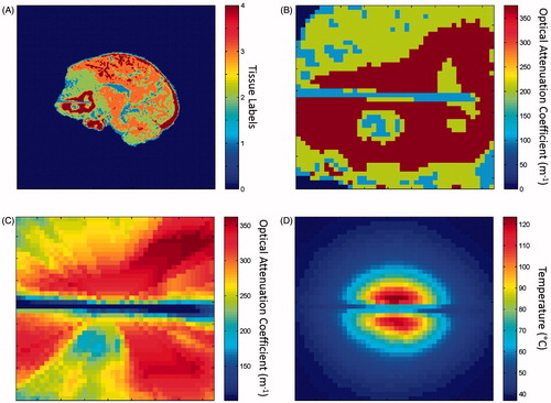
Table 1. Summary statistics for the tissue labels on T1W images.

	Tissue 1	Tissue 2	Tissue 3	Tissue 4
Mean	0.19	0.49	0.64	0.90
Std. dev.	0.10	0.05	0.04	0.08
Min.	0.00	0.36	0.58	0.71
Max.	0.36	0.58	0.79	1.00

Physics-based model of thermal ablation

Pennes bioheat equation

The steady-state Pennes bioheat equation [45] is used to estimate the temperature field induced by MRgLITT. This is a partial differential equation that models the heat transfer in tissue:

Here, u(x) is the temperature at spatial location x. The tissue properties λ, c_blood and ω represent thermal conductivity, blood-specific heat capacity and perfusion rate, respectively. Q_laser is the source term resulting from modelling of laser heating as the spherically symmetric solution to the photon transport equation in tissue [46]. The blood temperature, u_a, is assumed to be 37 °C in the human body. Active cooling of the laser fibre, u_D=22°C, is modelled by boundary conditions at the laser-tissue interface, ∂Ω_D. The laser source term, Q_laser, is a function of the effective optical attenuation coefficient, μ. Previous sensitivity analysis demonstrated the optical attenuation coefficient to have the largest influence on the temperature prediction [37]. Thus, tissue heterogeneity within the optical attenuation coefficient was examined in the present study. Tissue heterogeneities are modelled by the piece-wise continuous function. in which N_tissue=4 is the total number of tissue types, μ_n is the optical attenuation coefficient for tissue n and Ω_n is the spatial domain of tissue n within the full domain Ω. The Ω_n subdomains are mutually disjoint. Consequently, the modelled optical attenuation coefficient μ(x) is a piece-wise continuous function of spatial location x. The model prediction process is depicted in Figure 1.

Source term in heterogeneous tissue

Line integrals of the optical attenuation from the laser source are used to model the photon attenuation in heterogeneous tissue in the following equation:

Here, U_tip is the general source volume, P is the applied power of the laser fibre and ξ is the source position within U_tip.

Analytical steady-state solution

The solution to the Pennes bioheat equation is approximated using a one-dimensional spherically symmetric radial decomposition in spherical coordinates [36]. This analytical solution models heating from one point source. To model the cylindrical geometry of the laser fibre, the heating is approximated as the linear superposition of 50 point sources equally spaced over 1 cm along the laser fibre axis. Model parameter values are selected from the literature and summarised in Table 2. The value listed for optical attenuation coefficient is the initial guess used during optimisation. The other parameters are held constant.

Table 2. Model parameter values taken from the literature [46–48,55].

		P [W]
0.527	6.0	10.5	180.0	3840

Optical attenuation coefficient, μ, is the initial guess used in optimisation. The rest of the parameters are held constant.

Optimization of model parameters

Objective function

The goal of optimisation is to train this model to generate the greatest spatial agreement between its predicted ablation and the measured ablation in the thermometry data. Because agreement is evaluated using the DSC, the objective function, F, that should be minimised is:

Here, the objective function uses a continuous form of the DSC given by in which M and P are vectorised measurements and prediction data, respectively, and |⋅| is the absolute value. Two-dimensional thermometry measurements (m_i,j) and ablation predictions (p_i,j) are vectorised such that the data order is preserved as follows:

Measured and predicted ablation zones are calculated by applying a logistic function to the measured and predicted temperature maps (T_M and T_P, respectively):

This results in a continuous approximation of the 57 °C threshold for thermal damage [38].

Of note is that when all elements of M and P are binary, the continuous form of the DSC reduces to the discrete definition of DSC:

However, this classical form of the DSC leads to a piece-wise constant objective function and is non-differentiable. The continuous form of the DSC was useful in our study for creating a continuous objective function for gradient-based optimisation using interior point methods [47].

Tissue-distance metric for computation of path-average parameters

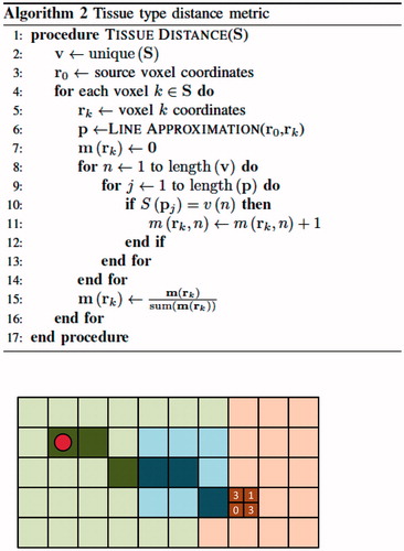
The heterogeneous optical properties being optimised vary in each iterative optimisation step. Repeated calculation of path-average optical attenuation coefficient values is computationally expensive. We employ a tissue-distance metric to reduce computational expense by pre-computing and storing the voxel-wise tissue-distance data required for repeated evaluation of the line integral (∫_r0^rkμ(s)ds). Bresenham’s line approximation is used to identify the voxels approximating the lines between the source voxel and all other voxels in the image. The algorithm for Bresenham’s line approximation and a simple example are shown in Figure 2. The inputs r₀ and r_k are the source and endpoint coordinates, respectively, of two points defining a line in discretized space, p_j are the coordinates of voxel j in the Bresenham’s line, d=r₀-r_k is the displacement vector and ϵ tracks increment movement in each direction. The source point, r₀, is placed at the centroid of the diffusing applicator. Along each line from source to endpoint, the fraction of voxels in each tissue label is stored and associated with the endpoint voxel. The algorithm for this tissue-distance calculation is shown in Figure 3, as well as a continuation of the example from Figure 2. The tissue-distance algorithm input S∈ℝ^N is an N-pixel discretized segmentation image or N-voxel volume of integer labels. The output is the tissue-distance metric m∈ℝ^N*4, where the ith row of m is the percent tissue label content of the linear path, s, from source r₀ to the ith pixel or voxel of S. If optical attenuation coefficients for the four tissue labels are given by the vector μ∈ℝ⁴, then the path-average optical attenuation coefficient, μ¯ ∈ ℝ^N, needed for computation of the source term is quickly calculated by μ¯=m× μ. This tissue-distance vector is a useful format for quick computation of average optical attenuation coefficient values between the source and all other points for variable optical attenuation coefficient values across all tissue types. As an example, consider a single line between the source and a distant point. Bresenham’s line approximation determines the straight line approximation between these points as a set of 20 voxels consisting of 2 voxels labelled grey matter, 10 voxels labelled white matter, 8 voxels labelled cerebrospinal fluid and 0 voxels labelled enhancing tumour. The tissue-distance vector for this endpoint voxel would be m=[m₁, m₂, m₃, m₄]=[0.1, 0.5, 0.4, 0]. If the optical attenuation coefficient vector for the different tissue types is μ =[μ₁, μ₂, μ₃, μ₄]=[160, 180, 200, 190], then the average optical attenuation coefficient seen across this line is the dot product of the tissue-distance vector and the optical attenuation coefficient vector, or 196. If μ is changed, then only the dot product of the tissue-distance vector and the optical attenuation coefficient vector needs to be repeated to obtain the path-average optical attenuation coefficient.

Figure 2. Example of two-dimensional Bresenham’s line approximation in heterogeneous tissue. The left (green), center (blue) and right (red) regions represent grey matter, an enhancing lesion and white matter, respectively. The line drawn from the source point to the end point is represented by seven pixels: three pixels classified as grey matter, three pixels classified as an enhancing tumour and one pixel classified as white matter.

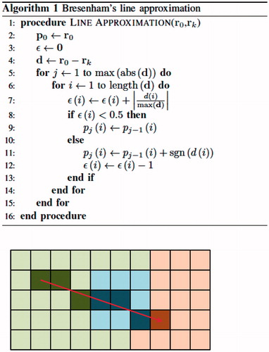
Figure 3. The tissue-distance metric for the line from the source to the example pixel shown in Figure 2. This path contains three grey matter labels, three enhancing lesion labels and one white matter label.

Multistart optimisation for heterogeneous tissue model

For the heterogeneous model, a multistart optimisation scheme was used to minimise the potential impact of local minima on the optimisation results due to noisy data. The optimised optical attenuation coefficient value for the homogeneous model, N_tissue=1, was used as one initial value in the multistart scheme for all four tissue types in each heterogeneous case. This provides a warm start for optimisation. Additional initial optical attenuation coefficient values are chosen in a 3 × 3×3 × 3 parameter-space grid centred on the homogeneous optimisation point with a distance of 5 m^-1 between adjacent points.

Evaluation of model overfit

Intuitively, an increased number of parameters for model optimisation is expected to lead to an improved objective function value and maximise predictive power of the model. However, additional unnecessary parameters will lead to model overfit. The potential overfit of the heterogeneous model optimisation results was normalised for the increased number of parameters using the Akaike Information Criterion (AIC) [48] and Bayesian Information Criterion (BIC) [49]. A logistic likelihood function, f(y|μ), was used to evaluate the data fit at the optimised values [50].

Here, pixel-wise values are assumed independent in the joint probability model encompassing the region of interest. AIC effectively normalises the log-likelihood by the number of parameters: one for the homogeneous model and four for the heterogeneous model. BIC further incorporates the number data points within the heating region of interest into the normalisation.

Cross-validation

Modeling prediction accuracy for MRgLITT is evaluated using leave-one-out cross-validation. This approach attempts to mimic the clinical scenario in which the thermometry data is not available for the case being tested. A population average over the 31 calibrated optical attenuation coefficients from each brain lesion ablation, excluding the case being tested, was used as the cross-validation optical attenuation coefficient

Cross-validation performance for case i is evaluated using DSC agreement with thermometry measurements, . The model-predicted ablation is generated using the cross-validation optical attenuation coefficient, A DSC equal to one indicates perfect coverage of the measured ablation region by the predicted ablation region. A DSC of zero represents complete separation of the two ablation regions.

To assess whether the median cross-validation DSC of the heterogeneous model is statistically different from that of the homogeneous model, we use a paired, two-tailed Wilcoxon signed-rank test. We perform the same test on calibration DSC values to determine whether the median calibration DSCs of the two models are statistically different.

Results

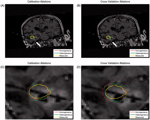
We trained the modelling prediction for MRgLITT using pre-treatment image data sets and MR thermometry data for the 31 ablations in the 22 unique patients. We quantitatively determined the accuracy of model predictions using the DSC between model-predicted and measured ablation regions (T > 57 °C) during both calibration and validation steps. The calibration and cross-validation performance for representative ablation predictions by the heterogeneous model and the homogeneous control model, as well as measured ablations from MR thermometry, are illustrated in Figure 4.

Figure 4. Representative model prediction performance. Both the homogeneous and heterogeneous model predictions of the ablation region, as well as the corresponding MR thermometry measurement, are overlaid on the T1W anatomy image. The performance is shown for model calibration (A), in which the homogeneous model DSC was 0.9344 and the heterogeneous model DSC was 0.9637, and for model cross-validation (B), in which the homogeneous model DSC was 0.8287 and the heterogeneous model DSC was 0.8560. The region of interest used in calibration (C) and cross-validation (D) calculations is also shown.

Calibration of both models results in a distribution of optimised optical attenuation coefficient values. Summary statistics for the homogeneous optimised optical parameter values and each tissue label for the heterogeneous model are provided in Table 3. Summary statistics for the corresponding intensity models that define each tissue label in T1W imaging are provided in Table 1.

Table 3. Summary statistics for optical attenuation coefficient calibration.

	Homogeneous tissue model	Heterogeneous tissue model
[m^-1]	Tissue 1	Tissue 1	Tissue 2	Tissue 3	Tissue 4
Mean	120.3	121.4	115.3	116.9	120.0
Median	112.0	114.0	112.3	112.6	114.0
Std. dev.	24.4	22.9	17.9	19.1	23.4
Min.	95.1	101.2	90.1	94.0	91.2
Max.	180.0	183.9	169.4	169.4	195.3

We used the population average of the calibrated optical attenuation coefficient values for each tissue label to retrospectively create predictive models from pre-treatment imaging. We evaluated the performance of these models using leave-one-out cross-validation with the 31 MR thermometry data sets. The calibration and cross-validation performance results are shown in Table 4. The median cross-validation DSC values for the homogeneous and heterogeneous models were 0.829 and 0.840, respectively.

Table 4. Summary of homogeneous and heterogeneous model performance in both calibration and cross-validation. The statistics given are for the distribution of DSC values between model-predicted and measured ablations in each of the 31 cases.

	Hom. calib.	Het. calib.	Hom. CV	Het. CV
Mean	0.842	0.874	0.753	0.763
Median	0.876	0.902	0.829	0.840
Std. dev.	0.127	0.089	0.177	0.170
Min.	0.367	0.549	0.259	0.283
Max.	0.968	0.968	0.945	0.964

Hom.: homogeneous; calib.: calibration; Het.: heterogeneous; CV: cross-validation.

A comparison of the calibration performance for the homogeneous and heterogeneous models is shown in Figure 5. The heterogeneous model had better calibration performance than the homogeneous model in 23 of the 31 cases. No cases were calibrated better with the homogeneous model. A similar comparison of cross-validation performance is shown in Figure 6. Seven cases performed better in cross-validation in the homogeneous model, whereas 23 cases performed better in the heterogeneous model. One case performed equally well in both models. Akaike and Bayesian information criteria values from each model calibration data is summarised in Table 5. Mean and median values for both AIC and BIC are smallest for the heterogeneous model. These results indicate that AIC and BIC prefer the heterogeneous model for calibration and the additional parameters for the heterogeneous model are unlikely to overfit the data.

Figure 5. Relative model calibration performance for the 31 brain lesion ablations. The values displayed are the differences between the heterogeneous and homogeneous model calibration DSCs. Positive values denote cases in which the heterogeneous model performed better than the homogeneous model did in calibration. The homogeneous model did not perform better in calibration in any case.

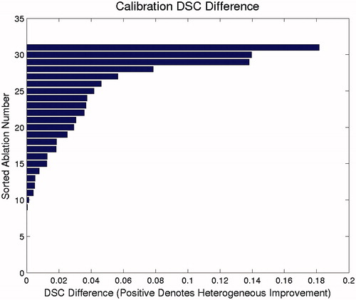
Figure 6. Relative model cross-validation performance for the 31 brain lesion ablations. The values displayed are the differences between the heterogeneous and homogeneous model cross-validation DSCs. Positive values denote cases in which the heterogeneous model performed better than the homogeneous model did in cross-validation, whereas negative values denote cases in which the homogeneous model performed better.

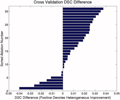
Table 5. Summary statistics for AIC and BIC model selection on the calibration data.

	Homogeneous tissue model		Heterogeneous tissue model
	AIC	BIC	AIC	BIC
Mean	538.0	543.4	193.0	214.5
Median	250.2	255.6	145.6	167.1

Results of a paired, two-tailed Wilcoxon signed-rank test regarding the calibration DSC for the homogeneous and heterogeneous models rejected the null hypothesis that the median heterogeneous DSC was lower than the median homogeneous DSC (p < 0.01). Thus, the calibration improvement for the heterogeneous model over that for the homogeneous model was statistically significant. Likewise, results of a paired, two-tailed Wilcoxon signed-rank test regarding the cross-validation DSC for the homogeneous and heterogeneous models rejected the null hypothesis that the median heterogeneous DSC was lower than the median homogeneous DSC (p < 0.01). Similarly, the cross-validation improvement for the heterogeneous model over that for the homogeneous model was statistically significant.

Discussion

We performed this study to model MRgLITT in heterogeneous tissue for the purpose of predicting the outcome of ablation of brain lesions. A sensitivity analysis [37] was used to identify that the optical parameters are expected to have the largest influence on the accuracy of the temperature prediction. Optimization of optical parameters using model degrees of freedom obtained via image segmentation represents a significant model reduction from using voxel-wise approaches [51]. Starting with initial optical parameter values in the literature [46,52], we accomplished highly accurate prediction of MRgLITT ablation by calibrating the steady-state Pennes bioheat equation to the available MR thermometry. The heterogeneous model demonstrated more accurate calibration than did the homogeneous control model. The additional modelling degrees of freedom afforded by the heterogeneous tissue enabled the ablation regions to better conform to tissue boundaries indicated in imaging. Therefore, our heterogeneous model exhibited promise in accurately predicting the shape and extent of ablations under difficult scenarios, such as near ventricle boundaries and large vessels. However, MR thermometry data on heating near these heat sinks were not available in the data set we used, which is a limitation of this study. We expect to see a larger difference in performance between the heterogeneous and homogeneous models in data sets with more ablations near heat sinks, but further work in larger patient cohorts is needed to calibrate and validate model predictions for MRgLITT near strong discontinuities of thermally and optically distinct tissue boundaries. In these scenarios, additional perfusion parameters may be warranted during the calibration step, and the trade-off between model overfitting and model prediction accuracy will need to be carefully studied. In addition to the AIC and BIC values, quantitative model selections approaches that compute the model plausibility [53] may also be considered in normalising the prediction performance by the model complexity.

Although cross-validation of models constructed from population-averaged parameters demonstrated that population-averaged parameters are likely to produce accurate models for treatment planning for MRgLITT, the predicted ablation boundary is highly affected by the imaging protocol and subsequent image segmentation agreement with thermally and optically distinct tissue boundaries. Also, variability in lesion enhancement will affect the segmentations and subsequent model parameters used. In order to begin with images registered to the MR thermometry data, the current preprocessing approach is to segment the T1W imaging used to locate laser fibres before MRgLITT begins. This approach should be extended and combined with diagnostic contrast-enhanced T1W imaging several days before MRgLITT. Our intent in using Gaussian mixture model segmentation with T1W imaging was to define the grey matter, white matter, cerebrospinal fluid and enhancing lesions on T1W images. However, the geometrical accuracy of these segmentations was not a focus of our study. Summary statistics for the imaging intensities (Table 1) effectively defined corresponding segmentation labels on the T1W images. The tissue segmentation approach to this normalised anatomical imaging enables the use of a quantitative and reproducible methodology for creating population models from the available calibration data. Variabilities in imaging protocol and lesion enhancement likely resulted in outliers in the calibrated parameter values, which were not modelled as well by the population average. This could explain the few cases where cross-validation performance did not improve for the heterogeneous model. Tissue segmentation from multiple pre-treatment images may be more robust to these variabilities. Higher order brain tumour segmentation methodologies [54] include T2W and fluid-attenuated inversion recovery imaging. These procedures may provide additional information in delineating tumour subvolumes.

Conclusion

In this study, we evaluated an outcome prediction model of MRgLITT for brain lesions, which simulates heterogeneous tissue, showing an improvement over simpler homogeneous tissue models [35,36]. Treatment planning for MRgLITT is currently performed by neurosurgeons, who review anatomical MR images and determine the laser fibre trajectory with the assistance of neuronavigation software. However, this methodology does not predict ablation outcomes during planning to evaluate possible trajectories. Researchers have accomplished this in the context of homogeneous tissue, but in practice, significant heterogeneities are found near critical structures and demand greater model complexity to accurately predict outcomes under these scenarios [36]. We accomplished more accurate MRgLITT outcome prediction by modelling four different tissue types with independent optical properties. This represents an important step toward development of commercialised MRgLITT treatment-planning programmes capable of improving pre-treatment planning and treatment quality.

Acknowledgements

The authors would like to thank Timothy J. Schaewe and Rebecca L. Vincelette for their insights into laser interstitial thermal therapy. We also thank the University of Texas MD Anderson Cancer Center Department of Scientific Publications for editing and proofreading.

Disclosure statement

No potential conflict of interest was reported by the authors.

Additional information

Funding

The research described herein was supported in part by Medtronic.

References

- Eichler K, Zangos S, Gruber-Rouh T, et al. (2014). MR-guided laser-induced thermotherapy (LITT) in patients with liver metastases of uveal melanoma. J Eur Acad Dermatol Venereol 28:1756–60.
- Patchell RA. (2003). The management of brain metastases. Cancer Treat Rev 29:533–40.
- Kalkanis SN, Linskey ME. (2010). Evidence-based clinical practice parameter guidelines for the treatment of patients with metastatic brain tumors: introduction. J Neurooncol 96:7–10.
- Gavrilovic IT, Posner JB. (2005). Brain metastases: epidemiology and pathophysiology. J Neurooncol 75:5–14.
- Owonikoko TK, Arbiser J, Zelnak A, et al. (2014). Current approaches to the treatment of metastatic brain tumours. Nat Rev Clin Oncol 11:203–22.
- Bafaloukos D, Gogas H. (2004). The treatment of brain metastases in melanoma patients. Cancer Treat Rev 30:515–20.
- Torres-Reveron J, Tomasiewicz HC, Shetty A, et al. (2013). Stereotactic laser-induced thermotherapy (LITT): a novel treatment for brain lesions regrowing after radiosurgery. J Neurooncol 113:495–503.
- Alexander E, Moriarty TM, Davis RB, et al. (1995). Stereotactic radiosurgery for the definitive, noninvasive treatment of brain metastases. J Natl Cancer Inst 87:34–40.
- Webb H, Lubner MG, Hinshaw JL. (2011). Thermal ablation. Semin Roentgenol 46:133–41.
- Kalkanis SN, Kondziolka D, Gaspar LE, et al. (2010). The role of surgical resection in the management of newly diagnosed brain metastases: a systematic review and evidence-based clinical practice guideline. J Neurooncol 96:33–43.
- Carpentier A, McNichols RJ, Stafford RJ, et al. (2011). Laser thermal therapy: real-time MRI-guided and computer-controlled procedures for metastatic brain tumors. Lasers Surg Med 43:943–50.
- Rieke R, Pauly KB. (2008). MR thermometry. J Magn Reson Imaging 27:376–90.
- McNichols RJ, Gowda A, Kangasniemi M, et al. (2004). MR thermometry-based feedback control of laser interstitial thermal therapy at 980 nm. Lasers Surg Med 34:48–55.
- Denis de Senneville B, Quesson B, Moonen CTW. (2005). Magnetic resonance temperature imaging. Int J Hyperthermia 21:515–31.
- Stafford RJ, Shetty A, Elliott AM, et al. (2010). Magnetic resonance guided, focal laser induced interstitial thermal therapy in a canine prostate model. J Urol 184:1514–20.
- Woodrum DA, Mynderse LA, Gorny KR, et al. (2011). 3.0T MR-guided laser ablation of a prostate cancer recurrence in the postsurgical prostate bed. J Vasc Interv Radiol 22:929–34.
- McDannold N, Tempany CM, Fennessy FM, et al. (2006). Uterine leiomyomas: MR imaging based thermometry and thermal dosimetry during focused ultrasound thermal ablation. RSNA Radiology 240:263–72.
- McNichols RJ, Kangasniemi M, Gowda A, et al. (2004). Technical developments for cerebral thermal treatment: water-cooled diffusing laser fibre tips and temperature-sensitive MRI using intersecting image planes. Int J Hyperthermia 20:45–56.
- Dewhirst MW, Viglianti BL, Lora-Michiels M, et al. (2003). Basic principles of thermal dosimetry and thermal thresholds for tissue damage from hyperthermia. J Int Hyperthermia 19:267–94.
- Stafford RJ, Fuentes D, Elliott AA, et al. (2010). Laser-induced thermal therapy for tumor ablation. Crit Rev Biomed Eng 38:79–100.
- Schulze PC, Vitzthum HE, Goldammer A, et al. (2004). Laser-induced thermotherapy of neoplastic lesions in the brain-underlying tissue alterations, MRI-monitoring and clinical applicability. Acta Neurochir 146:803–12.
- Carpentier A, Chauvet D, Reina V, et al. (2012). MR-guided laser-induced thermal therapy (LITT) for recurrent glioblastomas. Lasers Surg Med 44:361–8.
- Carpentier A, McNichols RJ, Stafford RJ, et al. (2008). Real-time magnetic resonance-guided laser thermal therapy for focal metastatic brain tumors. Neurosurgery 63:21–9.
- Norred SE, Johnson JA. (2014). Magnetic resonance-guided laser induced thermal therapy for glioblastoma multiforme: a review. Biomed Res Int 2014:761312. DOI:10.1155/2014/761312
- Schwarzmaier HF, Eickmeyer F, von Tempelhoff W, et al. (2006). MR-guided laser-induced interstitial thermotherapy of recurrent glioblastoma multiforme: preliminary results in 16 patients. Eur J Radiol 59:208–15.
- Schwarzmaier HJ, Eickmeyer F, Fiedler VU, Ulrich F. (2002). Basic principles of laser induced interstitial thermotherapy in brain tumors. Med Laser Appl 17:147–58.
- Jethwa PR, Barrese JC, Gowda A, et al. (2012). Magnetic resonance thermometry-guided laser-induced thermal therapy for intracranial neoplasms: initial experience. Neurosurgery 71:133–45.
- Anzai Y, Lufkin R, DeSalles A, et al. (1995). Preliminary experience with MR-guided thermal ablation of brain tumors. AJNR Am J Neuroradiol 16:39–52.
- Rahmathulla G, Recinos PF, Valerio JE, et al. (2012). Laser interstitial thermal therapy for focal cerebral radiation necrosis: a case report and literature review. Stereotact Funct Neurosurg 90:192–200.
- Nowell M, Miserocchi A, McEvoy AW, Duncan JS. (2014). Advances in epilepsy surgery. J Neurol Neurosurg Psychiatry 85:1273–9.
- Curry DJ, Gowda A, McNichols RJ, Wilfong AA. (2012). MR-guided stereotactic laser ablation of epileptogenic foci in children. Epilepsy Behav 24:408–14.
- Chen JC, Moriarty JA, Derbyshire JA, et al. (2000). Prostate cancer: MR imaging and thermometry during microwave thermal ablation-initial experience. Radiology 214:290–7.
- Rhim H, Dodd GD. (1999). Radiofrequency thermal ablation of liver tumors. J Clin Ultrasound 27:221–9.
- Simon CJ, Dupuy DE. (2006). Percutaneous minimally invasive therapies in the treatment of bone tumors: thermal ablation. Semin Musculoskelet Radiol 10:137–44.
- Fahrenholtz S, Madankan R, Danish S, Hazle JD, Stafford RJ, Fuentes D. (2018). Theoretical model for laser ablation outcome predictions in brain: calibration and validation on clinical MR thermometry images. J Int Hyperthermia 34:101–11.
- Fahrenholtz S, Moon T, Franco M, et al. (2015). A model evaluation study for treatment planning of laser induced thermal therapy. J Int Hyperthermia 0:1–32.
- Fahrenholtz SJ, Stafford RJ, Maier F, et al. (2013). Generalised polynomial chaos-based uncertainty quantification for planning MRgLITT procedures. J Int Hyperthermia 29:324–35.
- Yung JP, Shetty A, Elliott A, et al. (2010). Quantitative comparison of thermal dose models in normal canine brain. Med Phys 37:5313–21.
- Arlot S, Celisse A. (2010). A survey of cross-validation procedures for model selection. Stat Surv 4:40–79.
- Geisser S. (1980). Predictive sample reuse techniques for censored data. Trab Estad Invest Oper 31:433–68.
- Browne M. (2000). Cross-validation methods. J Math Psychol 44:108–32.
- Kohavi R. (1995). A study of cross-validation and bootstrap for accuracy estimation and model selection. Int Joint Conf Artif Intell 14:1137–43.
- Stafford RJ, Price RE, Diederich CJ, et al. (2004). Interleaved echo-planar imaging for fast multiplanar magnetic resonance temperature imaging of ultrasound thermal ablation therapy. J Magn Reson Imaging 20:706–14.
- Avants BB, Tustison NG, Wu J, et al. (2011). An open source multivariate framework for n-tissue segmentation with evaluation on public data. Neuroinformatics 9:381–400.
- Pennes H. (1948). Analysis of tissue and arterial blood temperatures in the resting human forearm. J Appl Physiol 1:93–122.
- Welch A. (1984). The thermal response of laser irradiated tissue. IEEE J Quantum Electron 20:1471–81.
- Wright S, Nocedal J. (1999). Numerical optimization. New York (NY), USA: Springer Science.
- Akaike H. (1981). Likelihood of a model and information criteria. J Econom 16:3–14.
- Posada D, Buckley TR. (2004). Model selection and model averaging in phylogenetics: advantages of Akaike information criterion and Bayesian approaches over likelihood ratio tests. Syst Biol 53:793–808.
- Sarkar SK, Habshah M, Rana S. (2010). Model selection in logistic regression and performance of its predictive ability. Aust J Basic and Appl Sci 4:5813–22.
- Fuentes D, Elliott A, Weinberg J, et al. (2013). An inverse problem approach to recovery of in vivo nanoparticle concentrations from thermal image monitoring of MR-guided laser induced thermal therapy. Ann Biomed Eng 41:100–11.
- Duck F. (1990). Physical properties of tissue: a comprehensive reference book. Cambridge (MA), USA: Academic Press.
- Cheung SH, Beck JL. (2010). Calculation of posterior probabilities for Bayesian model class assessment and averaging from posterior samples based on dynamic system data. Comput Aided Civ Infrastruct Eng 25:304–21.
- Menze BH, Jakab A, Bauer S, et al. (2015). The multimodal brain tumor image segmentation benchmark (brats). IEEE Trans Med Imaging 34:1993–2024.
- Diller KR, Valvano JW, Pearce JA. (2005). Bioheat transfer. In: Kreith F, Goswami Y, eds. The CRC handbook of mechanical engineering. 2nd ed. Boca Raton (FL), USA: CRC Press, 278–357.