Comparison between single- and dual-porosity models for fluid transport in predicting lesion volume following saline-infused radiofrequency ablation

Abstract

A recent study by Ooi and Ooi (EH Ooi, ET Ooi, Mass transport in biological tissues: Comparisons between single- and dual-porosity models in the context of saline-infused radiofrequency ablation, Applied Mathematical Modelling, 2017, 41, 271-284) has shown that single-porosity (SP) models for describing fluid transport in biological tissues significantly underestimate the fluid penetration depth when compared to dual-porosity (DP) models. This has raised some concerns on whether the SP model, when coupled with models of radiofrequency ablation (RFA) to simulate saline-infused RFA, could lead to an underestimation of the coagulation size. This paper compares the coagulation volumes obtained following saline-infused RFA predicted based on the SP and DP models for fluid transport. Results showed that the SP model predicted coagulation zones that are consistently 0.5 to 0.9 times smaller than that of DP model. This may be explained by the low permeability value of the tissue interstitial space, which causes the majority of the saline to flow through the vasculature. The absence of fluid flow tracking in the vasculature in the SP model meant that any flow of saline into the vasculature is treated as losses and do not contribute to the saline penetration depth of the tissue. Comparisons with experimental results from the literature revealed that the DP models predicted coagulation zone sizes that are closer to the experimental values than the SP models. This supports the hypothesis that the SP model is a poor choice for simulating the outcome of saline-infused RFA.

Keywords:

• Saline-infused RFA
• lesion size
• thermal ablation
• porous medium
• fluid transport

Introduction

Radiofrequency ablation (RFA) for cancer treatment is a technique that utilises heat to destroy cancer tissues and is predominantly used for treating liver cancer. RFA is based on the principle of Joule heating, a phenomenon in which the passage of an electric current through a material with finite conductivity, converts electromagnetic energy to heat through resistive losses in the material. In a typical RFA treatment, an electrode in the form of a needle-like probe is inserted percutaneously into the cancer tissue with the aid of a medical imaging technique, from where electrical current flows to grounding pads established onto the patient (usually at the thigh). Resistive heating causes the tissue temperature to rise and subsequently denaturate at temperatures of approximately 45 °C [1]. The denaturation process initiates necrosis and the cancerous tissue is eventually destroyed by way of hyperthermia.

Among the complexities and challenges associated with RFA are the tendency for tissue desiccation as a result of cellular water content vapourisation, and charring. Both of these complexities give rise to a limitation of treatable tumour size using RFA, since most of thermal damage happens adjacent to the probe. The presence of water vapour and charring around the probe increases the overall tissue impedance. This inhibits the flow of electric current further into the tissue; thus resulting in a reduced coagulation zone size. Popular methods for counteracting tissue vapourisation are infusion of the tumour with saline [2], the use of a cooled-tip probe [3,4], the application of RFA at various sites of the tumour [5] and the use of multi-tined electrodes [6,7]. These techniques may be used independently or adjuvant to each other. Saline infusion is typically performed via a modified probe that has infusion holes through which saline flows into the tissue. The aim of saline infusion is to increase the electrical conductivity of the liver tissue, allowing for enhanced resistive heating and subsequently the formation of larger coagulation zones. Meanwhile, internal circulation within cool-tip probes acts as a heat sink to regulate the temperature of tissue adjacent to the probe; hence, maintaining a low tissue impedance throughout.

One of the major hurdles when implementing saline-infused RFA is the difficulty in controlling and predicting the path of saline flow inside the tissue. An uncontrolled saline flow may lead to complications such as unintended ablation of the surrounding healthy tissues due to saline extravasation and jejunal perforation [8]. As such, the ability to monitor and to predict the pathway of saline remains a significant challenge that must be overcome for the successful clinical implementation of this technique. The difficulty in visualising fluid transport in vivo has resulted in mathematical and computational modelling techniques becoming viable options for researchers to investigate the flow dynamics inside biological tissues. Nevertheless, as with all computational models, especially those of biological systems, the model must faithfully replicate material properties and behaviour of the actual conditions associated with RFA.

Baxter and Jain [9,10] presented one of the earliest models for describing fluid flow inside biological tissues. In their model, the tissue interstitium is assumed to be porous, where the cells and the interstitial space are defined by the solid matrix and the pores of the porous medium, respectively. Fluid flow occurs through the pores of the tissue and is governed by the Darcy equation, while the hydraulic interaction between the interstitium and the vasculature and lymphatics is described based on the Kedem–Katchalsky theory [11]. Solute transport inside the tissue is modelled using the convection-diffusion equation, where the fluid exchange between the interstitium and the vasculature and lymphatics is described using properly formulated sources and sinks. One may consider the model proposed by Baxter and Jain [9,10] as a single-porosity (SP) representation of tissues due to the interstitium being considered as the only porous domain of interest. The majority of the studies on fluid flow in biological tissues have elected to use the SP model [12–14], perhaps due to its simplicity. Unfortunately, biological tissues, in particular the liver, consists of a highly complex network of blood vessels and lymphatics that reside within the same domain as the interstitium. Both components contribute to the transport characteristics of saline flow through the tissue. Therefore, the omission of the vasculature from the solution space will inadvertently result in a modest estimation of saline penetration into the tissue. In turn, this may influence the resulting predicted coagulation zone size.

By adding a vasculature component to the porous medium, a closer approximation of the actual saline penetration may be observed. This is the essence of the dual-porosity (DP) approximation, where both the interstitium and the vasculature are assumed to be porous domains that co-exist within the same space. Within the vasculature, the blood capillaries through which blood flows, are represented by the pores, while the voids among the capillaries are represented by the solid matrix. With DP models, the transport of fluid and solute in both the interstitium and the vasculature are explicitly monitored. This provides a more accurate representation of the flow dynamics inside biological tissues, since variation in the local pressure and solute concentration inside the interstitium and vasculature are taken into consideration. A number of researchers have adopted the DP model for studying fluid flow in biological tissues recently [15–18], albeit not from the context of saline-infused RFA. Conceivably, this has raised some questions on whether the SP or DP models would be the better model for describing saline transport when modelling saline-infused RFA. Burdío et al. [19] performed CT mapping of saline distribution inside the liver in vivo and found a tendency for saline to flow through the vasculature. More recently, Ooi and Ooi [20] performed a comparative study of the saline penetration depth estimated from both the SP and DP models. They found that the DP model predicted values that are approximately four times that of the SP model. These studies suggest that the SP model may not be the better choice due to the vasculature not being considered as part of the solution domain. Ooi and Ooi [20] further postulated that the smaller penetration depth predicted by the SP model may lead to predictions of smaller coagulation zones during saline-infuse RFA.

In this paper, we extend the investigations of Ooi and Ooi [20] by comparing the coagulation volumes obtained following saline-infused RFA based on the saline penetration depth predicted from SP and DP models. The main objective of this study is to determine whether the smaller penetration depth of saline predicted from SP models will translate to coagulation zones that are smaller than those of DP models when coupled with models of RFA. Given that the flow of saline is dictated by the hydraulic conductivity of the interstitium and the vasculature, the present study also investigates whether the use of the vascular hydraulic conductivity to replace that of the interstitium in the SP model can lead to solutions that approximate that of the DP model. This is crucial as the DP model is inherently more complex and more difficult to solve.

Materials and method

Investigations are carried out numerically using the commercial finite element software COMSOL Multiphysics^®. Two protocols for implementing saline-infused RFA are considered, namely infusion prior to ablation (pre-infusion) and infusion during ablation (simultaneous-infusion). The electrical potential and temperature distribution inside the tissue during RFA are governed by the quasi-static Maxwell equation and the Pennes bioheat equation, respectively. Formation of coagulation zone due to thermal insult is estimated based on the well-established Arrhenius thermal damage model. To ensure accuracy of the predictions, modelling parameters such as damage-dependent blood perfusion, temperature- and concentration-dependent electrical conductivity, temperature-dependent thermal conductivity and phase change effect to account for tissue vapourisation, are taken into account during the simulations. In order to verify whether the SP or DP model is more accurate, comparisons are carried out against ex vivo experimental studies reported in the literature.

Model geometry

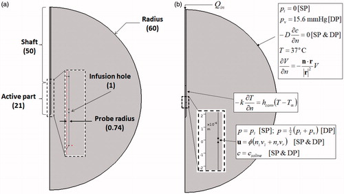
Figure 1(a) illustrates the model geometry used in the present study. The human liver is modelled as a sphere of radius 60 mm and is represented by a semicircle in 2 D axisymmetric coordinates. Preliminary investigations revealed that the size of 60 mm was sufficiently large to negate any boundary effects due to the selected truncated domain. A cooled-wet RF probe [21] of radius 0.74 mm (17 G needle) is inserted into the tissue from the top along the axis of symmetry. The probe has an active length of 21 mm, while the non-active part (shaft) is electrically insulated. Saline infusion is carried out from a hole of length $3\times {10}^{-4}$ mm located at the centre of the active part. This follows the numerical model of Trujillo et al. [22], which was adapted from the actual probe used by Ni et al. [21] and Cha et al. [23].

Figure 1. (a) Geometry and dimensions of the liver model used in this study (the dimensions in brackets are in mm) and (b) the boundary conditions implemented. The red point in (b) indicates the point where the temperature is probed for the implementation of the PID controller.

Governing equations

Single porosity model

As mentioned earlier, the SP model assumes the tissue as the only porous domain. The velocity of saline flowing through the interstitium can be described using the Darcy equation: (1) $$u=-\frac{{\kappa }_i}{\mu }\nabla p_i,$$(1) where $p_i$ is interstitial pressure, κ_i is the permeability of interstitium and μ is the dynamic viscosity of saline. Applying the continuity equation to Equation (1)(1) $$u=-\frac{{\kappa }_i}{\mu }\nabla p_i,$$(1) and accounting for the fluid exchange between the interstitial space and the vasculature and lymphatics by means of the Kedem–Katchalsky theory [11], one obtains: (2) $$\nabla ·\left(\frac{{\kappa }_i}{\mu }\nabla p_i\right)={\Theta }_v-{\Theta }_L,$$(2) where Θ_v and Θ_L are source and sink terms given by [9,20]: (3) $${\Theta }_v=\frac{L_{p,v}{S}_v}{V}\left[p_v-p_i-{\sigma }_t\left({\pi }_v-{\pi }_i\right)\right],$$(3) (4) $${\Theta }_L=\text{max}\left[\frac{L_{p,L}{S}_L}{V}\left(p_i-p_L\right),0\right],$$(4) where L_p is the hydraulic conductivity, $\frac{S}{V}$ is the surface area per unit volume, π is the osmotic pressure and σ_t is the osmotic reflection coefficient. The subscripts “$v$”, “$L$” and “$i$” represents vasculature, lymphatics and interstitium, respectively. The “max” operator in Equation (4)(4) $${\Theta }_L=\text{max}\left[\frac{L_{p,L}{S}_L}{V}\left(p_i-p_L\right),0\right],$$(4) simulates the presence of intraluminal valves within the lymphatic system that prevents backflow of saline into the interstitium [24].

The saline concentration distribution inside the tissue is described using the convection-diffusion equation [9]: (5) $$\frac{\partial c_i}{\partial t}+v_i·\nabla c_i=\nabla ·\left(D_i\nabla c_i\right)+{\Theta }_s-{\Theta }_L(c_{pl}-c_i)$$(5) where $c_i$ is the concentration of saline inside the interstitium, $v_i=\frac{u}{\varphi }$ is the interstitial saline velocity with $\varphi$ representing tissue porosity and $D_i$ is the saline diffusion coefficient inside the interstitium. Θ_s is a source term describing the transport of saline through the walls of the vasculature: (6) $${\Theta }_s={\Theta }_v(1-{\sigma }_f)\left|\frac{c_{pl}-c_i}{2}\right|+\frac{P_v{S}_v}{V}\left(c_{pl}-c_i\right),$$(6) where σ_f is the solute retardation coefficient as it passes through the vessel wall, $c_{pl}$ is the concentration of saline in plasma, $P_v$ is the vascular permeability coefficient, $\left|\frac{c_{pl}-c_i}{2}\right|$ approximates the mean mole fraction of saline within the pores [25] and Θ_L describes the loss of saline through the lymphatics and is given by Equation (4)(4) $${\Theta }_L=\text{max}\left[\frac{L_{p,L}{S}_L}{V}\left(p_i-p_L\right),0\right],$$(4) .

Dual porosity model

The DP model assumes the existence of two overlapping porous domains; that is, the interstitium and the vasculature. The equations governing the pressure inside the interstitium is identical to Equations (1(1) $$u=-\frac{{\kappa }_i}{\mu }\nabla p_i,$$(1) and 2(2) $$\nabla ·\left(\frac{{\kappa }_i}{\mu }\nabla p_i\right)={\Theta }_v-{\Theta }_L,$$(2) ); hence, they will not be repeated here. Across the vasculature, the equation governing the pressure distribution is given by: (7) $$\nabla ·\left(\frac{{\kappa }_v}{\mu }\nabla p_v\right)=-{\Theta }_v,$$(7) where ${\kappa }_v$ is the permeability of saline in the vasculature. The positive and negative signs preceding the term Θ_v in Equations (2(2) $$\nabla ·\left(\frac{{\kappa }_i}{\mu }\nabla p_i\right)={\Theta }_v-{\Theta }_L,$$(2) and 7(7) $$\nabla ·\left(\frac{{\kappa }_v}{\mu }\nabla p_v\right)=-{\Theta }_v,$$(7) ) ensures conservation of mass between both continua. The absence of Θ_L from Equation (7)(7) $$\nabla ·\left(\frac{{\kappa }_v}{\mu }\nabla p_v\right)=-{\Theta }_v,$$(7) implies that there is no transfer of fluid between the vasculature and the lymphatics. The convection-diffusion equation describing solute transport in the DP model for the interstitium is given by: (8) $$\frac{\partial c_i}{\partial t}+v_i·\nabla c_i=\nabla ·\left(D_i\nabla c_i\right)-\frac{F_s-F_L}{w_i},$$(8) and for the vasculature: (9) $$\frac{\partial c_v}{\partial t}+v_v·\nabla c_v=\nabla ·\left(D_v\nabla c_v\right)+\frac{F_s}{w_v},$$(9) where the variables with the subscript “$v$” correspond to the physical properties pertaining to the vasculature. The term $F_s$ describes solute transport between the interstitium and the vasculature and is given by [25]: (10) $$F_s={\Theta }_v(1-{\sigma }_f)\left(\frac{c_v-c_i}{2}\right)+\frac{P_v{S}_v}{V}\left(c_v-c_i\right).$$(10)

Similarly, the term $F_L$ describes solute transport between the interstitium and the lymphatics, and is given by: (11) $$F_L={\Theta }_L{c}_i,$$(11) where Θ_L is expressed as in Equation (4)(4) $${\Theta }_L=\text{max}\left[\frac{L_{p,L}{S}_L}{V}\left(p_i-p_L\right),0\right],$$(4) .

The laminar flow model

The flow of saline inside the probe is assumed to be laminar and incompressible. Ignoring the existence of body forces, the equation governing the flow of saline is described using the Navier-Stokes equations: (12) $$v_s·\nabla v_s=-\frac{1}{{\rho }_s}\nabla p+\frac{{\mu }_s}{{\rho }_s}{\nabla }^2{v}_s,$$(12) (13) $$\nabla ·v_s=0,$$(13) where v_s is the velocity vector, ρ_s and μ_s are the density and the dynamic viscosity of saline, respectively and $p$ is pressure.

The electrical potential model

For the range of frequency used in RFA (∼500 kHz), the electrical potential distribution inside the tissue during RFA is described using the quasistatic approximation of the Maxwell equations [26]: (14) $$\nabla ·\left(\sigma \nabla V\right)=0,$$(14) where σ is the tissue electrical conductivity and V is the electrical potential.

Bioheat transfer model

The transient temperature distribution inside the tissue during RFA is described using the Pennes bioheat equation [27]: (15) $$\rho c\frac{\partial T}{\partial t}+\rho c\left(v\nabla T\right)=\nabla ·\left(k\nabla T\right)+{\rho }_b{c}_b\omega \left(T_b-T\right)+q_{rfa},$$(15) where ρ, $c$ and $k$ are the tissue density, specific heat and thermal conductivity, respectively, v is the velocity vector of saline inside the tissue (vasculature in the case of the DP model), $T$ is temperature, $t$ is time, ω is the blood perfusion rate, ρ_b is the blood density, $c_b$ is the specific heat of blood and $q_{rfa}$ is the heat generated due to resistive heating given by: (16) $$q_{rfa}=\sigma {\left|\nabla V\right|}^2.$$(16)

During ablation, some parts of the tissue may experience temperatures beyond 100 °C, in which case, tissue vapourisation will occur. To account for the thermal effects due to phase change, the apparent heat capacity method is employed [28]: (17) $${\left(\rho c\right)}_{app}=\{\begin{array}{ll}\begin{array}{l}\rho c,\hfill \\ \frac{\rho c+{\left(\rho c\right)}_{vqp}}{2}+\frac{{\rho }_w{h}_{fg}\beta }{T_u-T_l},\hfill \\ {\left(\rho c\right)}_{vap},\hfill \end{array}\hfill & \begin{array}{l}T\le T_l\hfill \\ T_l<T\le T_u\hfill \\ T>T_u,\hfill \end{array}\hfill \end{array}$$(17) where the subscripts “$vap$” and “$w$” represent vapour and water, respectively, $h_{fg}$ is the latent heat of vapourisation, β is the tissue water content, and $T_l$ and $T_u$ are the lower and upper temperatures of the phase change process given by 99 °C and 100 °C, respectively. Equation (17)(17) $${\left(\rho c\right)}_{app}=\{\begin{array}{ll}\begin{array}{l}\rho c,\hfill \\ \frac{\rho c+{\left(\rho c\right)}_{vqp}}{2}+\frac{{\rho }_w{h}_{fg}\beta }{T_u-T_l},\hfill \\ {\left(\rho c\right)}_{vap},\hfill \end{array}\hfill & \begin{array}{l}T\le T_l\hfill \\ T_l<T\le T_u\hfill \\ T>T_u,\hfill \end{array}\hfill \end{array}$$(17) is substituted into the first term on the left-hand-side of Equation (15)(15) $$\rho c\frac{\partial T}{\partial t}+\rho c\left(v\nabla T\right)=\nabla ·\left(k\nabla T\right)+{\rho }_b{c}_b\omega \left(T_b-T\right)+q_{rfa},$$(15) .

Cell death model

The coagulation zone formed during RFA signifies zone of cell death, which in this study, is modelled using the well-established Arrhenius equation: (18) $$\Omega (r,t)=A{\displaystyle \int \exp }\left(-\frac{\Delta E}{RT(r,t)}\right)dt,$$(18) where Ω is a parameter that quantifies the amount of thermal damage inside the tissue, $A$ is the frequency factor, $\Delta E$ is the activation energy representing irreversible thermal energy damage reaction and $R$ is the universal gas constant.

Initial-boundary conditions

The initial-boundary conditions used in the present study are depicted in Figure 1(b).

Laminar flow model

The laminar flow model is active only in the domain representing the probe. At the top boundary, a fully developed laminar flow profile calculated for a constant saline flow rate of $Q_{in}$ and an entrance length of 0.19 m is prescribed. The entrance length was selected by ensuring that its value is significantly greater than 0.06 $ReD$, where $Re$ is the Reynolds number and $D$ is the hydraulic diameter. This is necessary to allow the flow of saline to adjust to a fully developed profile. The saline infusion hole represents the interface boundary between the needle and the tissue. A matching pressure condition is prescribed here. For the SP model, the pressure at the infusion hole is set to be the same as the pressure at the interstitium. For the DP model, the pressure is set to be the average of the vascular and interstitial pressure. Stationary no slip wall condition is set across all the remaining boundaries.

Single porosity model

A zero interstitial pressure and an outflow boundary condition defined by ($-D_i\nabla c_i·n=0$) is prescribed at the outer boundaries of the tissue to mimic the pressure and outflow of saline at the far-field, respectively. At the infusion boundary, an inlet velocity matching the outlet velocity of saline from the needle is prescribed. The concentration here is set to $c_i=c_{saline}$ to mimic the infusion of saline. The initial concentration is set to $c_i=c_{pl}$, where $c_{pl}$ is the physiological saline concentration inside biological tissues.

Dual porosity model

With the DP model, the boundary conditions used to describe the interstitium are similar to those used in the SP model. At the outer boundaries, a constant vascular pressure of $p_v=15.6$ mmHg and an outflow condition of $-D_v\nabla c_v·n=0$ is prescribed. The former mimics the vascular pressure at the far-field. At the infusion site, the Dirichlet condition of $c_v=c_s$ is prescribed. The initial concentration across the vasculature is set to c_v = c_pl.

Electrical potential field

Across the active part of the probe, a time-dependent electrical potential defined by $V=V_{app}(t)$ is prescribed. The variation with time is due to the implementation of the temperature-regulated protocol. Across the outer boundaries, the Robin condition defined by [13]: (19) $$\sigma \frac{\partial V}{\partial n}=-\frac{n·r}{{\left|r\right|}^2}V,$$(19) is prescribed, where r is the position vector and n is the unit normal vector pointing outwards from the outer tissue surface. Equation (19)(19) $$\sigma \frac{\partial V}{\partial n}=-\frac{n·r}{{\left|r\right|}^2}V,$$(19) ensures that the electrical current flows radially and smoothly towards the distant surface. All other boundaries are electrically insulated.

The thermal field

The initial temperature is set to be 37 °C. This value is also prescribed across the outer boundaries by assuming the domain to be sufficiently large for the surrounding blood flow to maintain the temperature here at basal level. At the boundary of the active part of the probe, the Robin condition defined by [29]: (20) $$-k\frac{\partial T}{\partial n}=h_{conv}\left(T-T_{\infty }\right),$$(20) is prescribed, where $h_{conv}$ is the convection heat transfer coefficient and $T_{\infty }$ is the temperature of the circulating liquid.

The cell death model

Since no tissue damage occurs prior to ablation, the initial condition of $\Omega (r,0)$ = 0 is set for the cell death model.

Model implementation

Tissue thermal conductivity

The thermal conductivity of the tissue is assumed to increase linearly with temperature according to the function [30]: (21) $$k(T)=\{\begin{array}{ll}{k}_o+\Delta k\left(T-T_{ref}\right),\hfill & T\le T_u\hfill \\ k_o+\Delta k\left(T_u-T_{ref}\right),\hfill & T>T_u\hfill \end{array},$$(21) where $k_o$ is the thermal conductivity measured at baseline temperature $T_{ref}$ and $\Delta k$ is the rate of increase of the tissue thermal conductivity with temperature.

Tissue electrical conductivity

The electrical conductivity of the tissue is assumed to be temperature- and concentration-dependent. For temperature dependence, the function proposed by Trujillo et al. [30] is used: (22) $$\sigma (T)=\{\begin{array}{ll}{\sigma }_o\left(1+\Delta \sigma (T-T_{ref})\right),\hfill & T\le T_u\hfill \\ \begin{array}{l}\frac{1}{5}\left[{\sigma }_{vap}-{\sigma }_o\left(1+\Delta \sigma (T_u-T_{ref})\right)\right]\left(T-T_u\right)\dots \hfill \\ +{\sigma }_o\left(1+\Delta \sigma (T_u-T_{ref})\right),\hfill \end{array}\hfill & T_u<T\le T_u+5\hfill \\ {\sigma }_{vap},\hfill & T>T_u+5\hfill \end{array},$$(22) where σ_o is the tissue electrical conductivity evaluated at baseline temperature $T_{ref},\Delta \sigma$ is the rate of increase of the tissue electrical conductivity against temperature and σ_vap is the electrical conductivity of vapour.

During saline-infused RFA, the tissue electrical conductivity will increase as a function of the local saline concentration. Here, it is assumed that the tissue electrical conductivity increases linearly with the concentration of saline. At basal concentration of $c_{pl}$ (when no saline has penetrated the tissue), the electrical conductivity is at baseline value. When the tissue is completely saturated with saline, the tissue electrical conductivity is assumed to have value that is similar to saline, i.e. approximately 12 times the value of tissue baseline [2]. Between the unsaturated and fully saturated cases, a linear increase in the tissue electrical conductivity is assumed. This can be expressed mathematically as [13]: (23) $$\sigma (c,T)=\{\begin{array}{ll}\sigma (T),\hfill & c\le c_{pl}\hfill \\ \sigma (T)\left[1+\frac{11}{20}\left(c-c_s\right)\right],\hfill & c_{pl}<c<c_s,\hfill \\ 12\sigma (T),\hfill & c\ge c_s\hfill \end{array},$$(23) where $\sigma (T)$ represents the temperature-dependent electrical conductivity given by Equation (22)(22) $$\sigma (T)=\{\begin{array}{ll}{\sigma }_o\left(1+\Delta \sigma (T-T_{ref})\right),\hfill & T\le T_u\hfill \\ \begin{array}{l}\frac{1}{5}\left[{\sigma }_{vap}-{\sigma }_o\left(1+\Delta \sigma (T_u-T_{ref})\right)\right]\left(T-T_u\right)\dots \hfill \\ +{\sigma }_o\left(1+\Delta \sigma (T_u-T_{ref})\right),\hfill \end{array}\hfill & T_u<T\le T_u+5\hfill \\ {\sigma }_{vap},\hfill & T>T_u+5\hfill \end{array},$$(22) . The variable $c$ in Equation (23)(23) $$\sigma (c,T)=\{\begin{array}{ll}\sigma (T),\hfill & c\le c_{pl}\hfill \\ \sigma (T)\left[1+\frac{11}{20}\left(c-c_s\right)\right],\hfill & c_{pl}<c<c_s,\hfill \\ 12\sigma (T),\hfill & c\ge c_s\hfill \end{array},$$(23) takes the value of the interstitium in the SP model and the value of the vasculature in the DP model.

Coagulation zone size

The parameter Ω in Equation (18)(18) $$\Omega (r,t)=A{\displaystyle \int \exp }\left(-\frac{\Delta E}{RT(r,t)}\right)dt,$$(18) represents the amount of damage sustained by the tissue due to thermal insult. According to Agah et al. [31], the value of Ω = 1 represents the onset of tissue coagulation. Hence, in this study, the coagulation zone size is determined by calculating the volume integral of the nodes with $\Omega >1$.

Damage-dependent blood perfusion rate

During ablation, heat causes the blood vessels to rupture and this results in the cessation of blood perfusion in parts of the tissue that are thermally-damaged. To account for this, a damage-dependent blood perfusion rate is prescribed. To quantify the thermally damaged region, the threshold used to define the coagulation zone, that is, $\Omega >1$, is adopted [31]. Hence, the damage-dependent blood perfusion rate is given by: (24) $$\omega (\Omega )=\{\begin{array}{c}{\omega }_b,\\ 0,\end{array}\begin{array}{c}\Omega \le 1\\ \Omega >1\end{array},$$(24) where ω_b is the baseline blood perfusion rate.

Impedance-controlled ablation

An impedance-controlled ablation protocol is assumed in the present study. In this protocol, a constant voltage of $V_{app}=$ 80 V is applied across the active part of the probe. The overall tissue impedance $Z$, measured as: (25) $$Z(t)={\displaystyle \underset{R}{\iint }\frac{V_{app}^2(t)}{Q_{tot}}}dR,$$(25) where $R$ is the domain representing the tissue and $Q_{tot}$ is the total RF energy absorbed by the tissue, is monitored at every time step. When the tissue impedance is 30 Ω above its initial value, ablation is halted for 20 s by setting $V_{app}=$ 0 V; after which the ablation process is restarted [32].

Material properties

All the material properties used in this study are sourced from the literature. Values representing that of the liver are used whenever they are available. Except for the electrical conductivity, thermal conductivity and blood perfusion rate, values of all the parameters used are assumed to be constants. These are summarised in Tables 1 and 2.

Table 1. Hydraulic and transport parameters used in the present study.

Parameter	Value	Source
Interstitial space permeability, κi (m^2)	3.12 × 10^–17	[15]
Vascular space permeability, ${\kappa }_v$ (m^2)	1.56 × 10^–14	[35]
Dynamic viscosity of saline, μ (Pa⋅s)	0.0007	[36]
Vasculature hydraulic conductivity, $L_{p,v}$ (m/(Pa⋅s))	5.68 × 10^–11	[15]
Vascular surface area to volume ratio, $S_v/V$ (1/m)	7000	[9]
Lymphatics transfer coefficient, Lp,LSL/V (Pa⋅s)^– 1	4.43 × 10^–9	[15]
Vascular pressure, $p_v$ (Pa)${}^{\text{a}}$	2080	[9]
Lymphatics pressure, $p_L$ (Pa)	133.3	[9]
Vascular osmotic pressure, πv (Pa)	2666.67	[9]
Interstitial fluid osmotic pressure, πi (Pa)	1333.33	[9]
Osmotic reflection coefficient, σT	0.91	[9]
Vascular permeability coefficient, $P_v$ (m/s)	7.3 × 10^–12	[9]
Vascular space diffusion coefficient, $D_v$ (m^2/s)	4.2 × 10^–10	[37]
Interstitial space diffusion coefficient, $D_i$ (m^2/s)	1 × 10^–9	[38]
Solute retardation coefficient, σsol	0.90	[9]
Volume fraction of vascular space, $w_v$	0.143	[35]
Volume fraction of interstitial space, $w_i$	0.857	1-$w_v$
Tissue porosity, ${\varphi }_i$	0.6	[39]
Vasculature porosity, ${\varphi }_v$	1	[25]
Saline concentration in plasma, $c_{pl}$ (mol/m^3)	134
Saline concentration, $c_s$ (mol/m^3)	154

^a Value is used only for the SP model.

Table 2. Thermal, electrical and cell death parameters used in the present study.

Parameter	Value	References
Electrical model
Baseline liver electrical conductivity, σ0 (S/m)	0.33	[40]
Vapour electrical conductivity, σvap (S/m)	0.001σ0
Probe electrical conductivity, σprobe (S/m)	10^8
Shaft electrical conductivity, σshaft (S/m)	4 × 10^6
Thermal model
Liver thermal conductivity, κ (W/m⋅K)	0.512	[40]
Liver density, ρ (kg/m^3)	1060
Liver heat capacity, C (J/kg⋅K)	3600
Probe thermal conductivity, κprobe (W/m⋅K)	18
Probe density, ρprobe (kg/m^3)	6450
Probe heat capacity, $C_{probe}$ (J/kg⋅K)	840
Shaft thermal conductivity, κshaft (W/m⋅K)	71
Shaft density, ρshaft (kg/m^3)	21 500
Shaft heat capacity, $C_{shaft}$ (J/kg⋅K)	132
Blood density, ρb (kg/m^3)	1000
Blood heat capacity, $C_b$ (J/kg⋅K)	4180
Baseline blood perfusion rate, ωb (1/s)	0.0064
Latent heat of vapourisation, $h_{fg}$ (J/kg)	2.26 × 10^6	Assumed as water
Tissue water content, β	0.71	[32]
Heat capacity of water vapour,  ${\left(\rho c\right)}_{vap}$ (J/m^3· K)	6 × 10^5
Cell death model
Frequency factor, A (1/s)	7.395 × 10^39	[41]
Activation energy, $\Delta E$ (J/mol)	2.5775 × 10^5
Universal gas constant, R (J/mol⋅K)	8.314

Mesh convergence

A mesh convergence study is necessary to determine the minimum number of elements required to achieve results that are independent of element size. Five points across the tissue are selected, where the temperatures here are monitored to decide if convergence has been achieved. To enforce a more stringent convergence test, the coagulation volume is also added as another parameter that is monitored. Triangular elements were used to discretize the model. Second order discretization was used in all the physics except for the Navier–Stokes equations, where linear discretization was selected in order to facilitate with the convergence of the numerical scheme. An adaptive time stepping scheme was used to determine the optimal time. Results from the mesh convergence study showed that increasing systematically the number of elements from 1720 to 26 175 led to percentage difference in the temperatures across the five sampling points of less than 1%, while the coagulation volume showed differences of less than 2%. The mesh setting resulting in 26 175 elements is thus used in all subsequent simulations.

Results

Pre-infusion of saline

In the pre-infusion protocol, saline is injected into the tissue as a bolus immediately before ablation. Five different saline volumes are investigated, namely 2.5, 5, 10, 15 and 20 ml. The infusion rate of saline was kept at 0.075 ml/min, following the proposal by Gilliams and Lees [8] on using low infusion rate. The infusion time was altered for each case to ensure that the correct amount of saline is infused into the tissue. This is followed by 10 min of ablation.

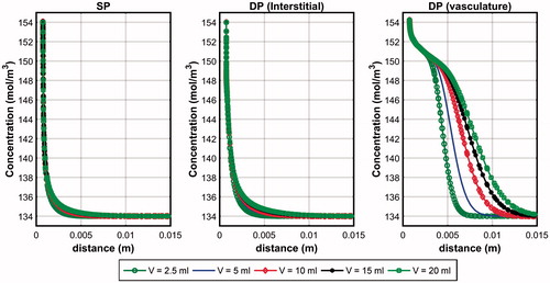
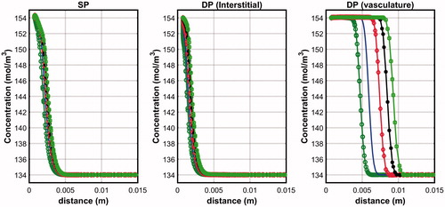
Figure 2 compares the penetration depth of saline along the horizontal line across the centre of the infusion hole at the end of infusion. For the DP model, plots across both the interstitium and the vasculature are shown. Both the SP and DP models predicted very low saline penetration depth across the interstitium with negligible effects observed when saline volume is increased. The SP model predicted a slightly smaller penetration depth than the DP model and this may be explained by the constant and homogeneous vascular pressure distribution assumption of the SP model. With the DP model, the local vascular pressure variation meant that some saline could re-enter the interstitium when the vascular pressure is greater than the interstitial pressure, and this happens usually at points that are further away from the infusion hole. The penetration depth across the vasculature is significantly higher than in the interstitium and this may be explained by the vasculature having a larger permeability value than the interstitium (Table 1). Since the DP model assumes the vasculature and the interstitium to occupy the same tissue space, the penetration depth across the vasculature may also be regarded as the overall penetration depth of the tissue. On the other hand, the tissue penetration depth of the SP model is simply the penetration depth through the interstitium. By arbitrarily taking 138 mol/m³ to define penetration depth [20], it was found that the DP model predicted saline penetration depths that are 4.7 to 7.6 times larger than that of the SP model.

Figure 2. Penetration depth of saline after 10 min of infusion in the SP and DP (interstitium and vasculature) models obtained for the pre-infusion mode.

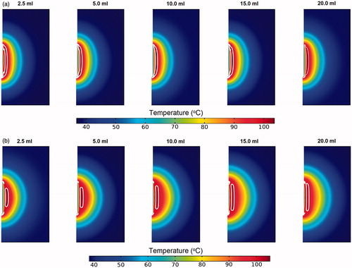
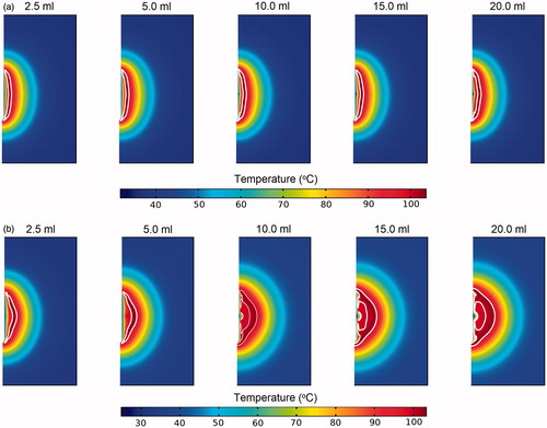
Figure 3 shows the temperature contours obtained from the SP and DP models at the time when the measured tissue temperature is at its maximum. Region enclosed by the white line represents zone with temperatures exceeding 99 °C, that is, the vapourisation zone. For the SP model (Figure 3(a)), the different infusion volumes were found to have insignificant effects on the tissue temperature distribution. This may be explained by the near identical saline penetration depth for the different infusion volumes, which limited the variation observed in the tissue temperature profile. The presence of vapourisation zone is apparent and appears as an elongated shape that covers the entire active region of the probe. With the DP model, as the volume of saline increases, the size of the vapourisation zone also increases and the shape becomes more elongated along the length of the probe. This phenomenon may be explained by the increase in the area with elevated electrical conductivity due to the presence of saline, which led to enhanced local tissue electrical conductivity and hence more intense resistive heating. In all the cases considered, the maximum temperature occurs at a distance away from the probe’s surface, which is characteristic of the cool-tip probe [3].

Figure 3. Contours of the temperature distribution 10 min after pre-infused RFA of the (a) SP and (b) DP models. Regions within the white lines represent zones where tissue vapourisation occurs.

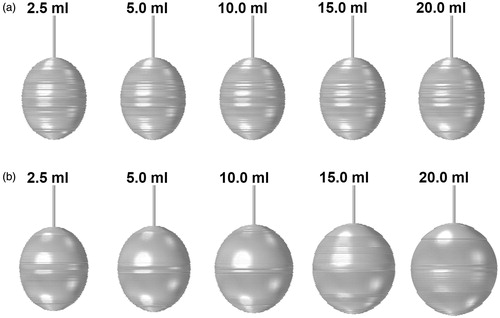
Figure 4 shows the rendering of the coagulation zones obtained for the different saline infusion volumes following 10 min of ablation. The corresponding volumes are tabulated in Table 3. From Figure 4, it can be observed that the coagulation zones predicted using the SP model appear thinner and elongated along the axial direction. Increasing the saline volume increases the coagulation size only very slightly, with the largest variation of 2.4% (Table 3). This coincided with the results obtained on the negligible impact of the saline volume on the tissue penetration depth (Figure 2). With the DP model, the coagulation zones obtained are larger and have a greater distance in the lateral direction. This may be explained by the large presence of saline inside the vascular space of the tissue estimated from the DP model. Increasing the volume of saline infusion increases the size of the coagulation zone. Overall, the DP model estimated coagulation zones that are 1.37 to 2 times larger than those obtained using the SP model, with the difference becoming larger as the volume of saline increases.

Figure 4. Coagulation zone formation following saline infused RFA with pre-infusion of saline obtained using the (a) SP and (b) DP models.

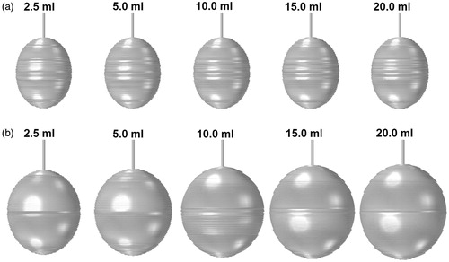
Table 3. Comparisons of the coagluation volumes (cm³) obtained using the SP, DP and SP (with vascular permeability) models.

	Pre-infusion			Simultaneous-infusion
Saline volume (ml)	SP	DP	SP (with κv)	SP	DP	SP (with κv)
2.5	26.01	35.74	27.78	25.48	29.05	28.86
5	26.64	41.03	28.62	25.75	32.97	31.91
10	27.16	48.79	29.53	26.11	38.81	32.65
15	27.45	53.20	30.85	26.39	44.56	34.14
20	28.09	56.29	31.37	26.66	48.26	36.87

Simultaneous infusion of saline

In the simultaneous infusion protocol, both saline infusion and RFA are carried out concurrently. As such, the infusion time and the ablation time are identical, that is, at 10 min. As in the pre-infusion case, five saline volumes are investigated, namely 2.5, 5, 10, 15 and 20 ml. Since the infusion time is fixed at 10 min, the infusion rate for each volume is altered accordingly so that the correct amount of saline is infused into the tissue at the end of ablation. Figure 5 plots the saline penetration depth predicted using the SP and DP models obtained for the simultaneous-infusion case. Unlike the pre-infusion mode, there is a larger penetration depth observed in both the predictions of the SP and DP models. This is due to the higher infusion rate assumed in the simultaneous infusion mode. In the pre-infusion mode, the infusion rate was set to 0.075 ml/min, while the infusion time was altered to deliver the proper amount of saline into the tissue. In the simultaneous infusion mode, the infusion time was set to 10 min to coincide with the ablation time, while the infusion rate was altered to achieve the correct volume of saline infused into the tissue.

Figure 5. Penetration depth of saline after 10 min of infusion in the SP and DP (interstitium and vasculature) models obtained for the simultaneous infusion mode. Color legend is similar to that in Figure 2.

Figure 6 shows the temperature contours across the tissue during the period when the measured tissue temperature is at its maximum. Similar to the pre-infusion case, there is very little variation in the temperature distribution of the SP model for the different infusion volumes considered. With the DP model, the zone of high temperature travels deeper into the tissue as the volume of saline increases. This naturally also means that the vapourisation zone travels deeper into the tissue, as indicated by the white lines in Figure 6(b). This observation may be explained by the increase in the convective currents when saline volume is increased. Since the present model restricts the ablation duration to 10 min, the increase in saline volume is defined by an increase in the saline infusion rate. Hence, an increase in saline volume also translates to more intense flow of saline into the tissue.

Figure 6. Contours of the temperature distribution 10 min after simultaneous-infused RFA of the SP and DP models. Regions within the white lines represent zones where tissue vapourisation occurs.

Figure 7 illustrates the rendering of the coagulation zones formed at the end of the ablation process for the SP and DP models, while the corresponding values of the coagulation zone volume are tabulated in Table 3. With the SP model, there is very little difference in the coagulation zone volume as the infusion volume is increased from 2.5 to 20 ml (maximum difference of 1.3%). With the DP model, increasing the saline volume increases the volume of the coagulation zone. Overall, the DP model estimated coagulation zones that are 1.14 to 1.81 times the coagulation zone predicted using the SP model. As in the pre-infusion case, the coagulation zone shapes predicted from the DP model have a profile that is more spherical than those of the SP model.

Figure 7. Coagulation zone formation following saline infused RFA with simultaneous-infusion of saline obtained using the SP and DP models.

Single porosity model with vascular permeability

Results from the above sections suggest that the coagulation zone size estimated from the SP and DP models are significantly different, with the DP model estimating coagulation zones that are larger than that of the SP model. As discussed earlier, it was hypothesised that it may be possible for the SP model to approximate the results of the DP model if the value of intersititial permeability is replaced with that of the vasculature. To test this hypothesis, simulations are repeated for both the pre-infusion and simultaneous-infusion cases using the SP model with the vascular permeability value in place of the interstitium. For simplicity, this is hereafter referred to as the new SP model. For the hypothesis to be tenable, the saline penetration depth and the coagulation zone volume and shape obtained with the new SP model must approach that of the DP model.

Figure 8 compares the saline penetration depths across the interstitium of the new SP model and those across the vasculature of the DP model obtained for both the pre-infusion and simultaneous-infusion modes. The corresponding plots for the SP and DP (vasculature only) models are also shown for comparison. In the pre-infusion mode, it can be seen that the new SP model predicted only a very small increase in the penetration depth when compared to the SP model. The penetration depth for the new SP model is significantly smaller than the estimates of the DP model, however. In the simultaneous-infusion mode, the new SP model predicted penetration depths that are significantly larger than the SP model. Nevertheless, there is still a 4.4 to 13.2% diffrerence when compared to the DP model.

Figure 8. Comparison between the saline penetration depth obtained using the new SP model and the DP model (vasculature only) for (a) pre-infusion and (b) simultaneous-infusion protocols. Colour legend is similar to that in Figure 2.

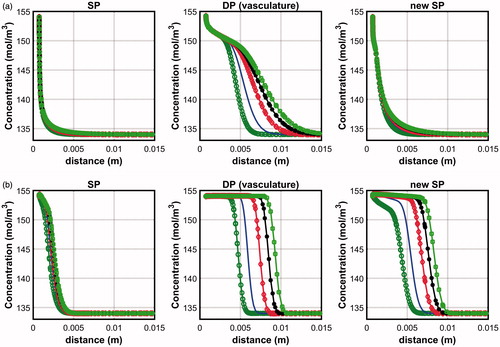
Table 3 presents the volume of the coagulation zone obtained for the new SP model for the pre-infusion and simultaneous infusion modes. In pre-infusion mode, the coagulation zone volume for the new SP model is 6.8% to 12.4% larger than those obtained for the SP model, but 22.3 to 44.3% smaller than the DP model, depending on the saline volume. In simultaneous infusion mode, the predictions of the new SP model is closer to the DP model, with percentage differences ranging from 0.6 to 23.6%; the difference becoming larger as the saline volume increases.

Comparisons with experimental results from the literature

In order to determine whether the SP or the DP models will approximate more closely the coagulation zone in an actual saline-infused RFA treatment, comparisons with experimental studies found in the literature are carried out. This is carried out against the work of Cha et al. [23] for ex vivo bovine livers, from which the present probe design is modelled. The models were set up to follow as close as possible the experimental settings adopted by these papers. These include parameters such as the volume of saline, the infusion rate, the duration of ablation and the dimensions of the probe; all of which were selected to match those used in the experiments. Furthermore, the models were adapted to account for the absence of the thermal and mass transport effects due to the absence of blood flow in ex vivo tissues. Simulations were carried out for the probes with 2 and 3 cm active length. It is important to note that in spite of the effort to match closely the experimental settings, there are some differences between the model and the experiments that make a one-to-one comparison difficult. Firstly, there are two infusion holes located at opposite sides of the actual electrode [23], while the present study considers only one infusion hole with the same infusion area located at the centre [33]. The deviation in the electrode design is necessary for the model to be developed in axisymmetric conditions. Secondly, the ablation protocol employed in the present study is different from that of the experiments. In the experiments, a maximum power output of 200 W is delivered to the tissue via an optimised algorithm. This was not prescribed in the present study due to the absence of a computational module in our COMSOL software that is required to perform such a task. As such, the delivery of RF energy in the present study is accomplished by prescribing a constant voltage across the active part of the electrode. Given these discrepancies, it is important to treat the comparisons presented in this section as purely qualitative rather than quantitative.

Table 4 compares the maximum diameter in the longitudinal and axial directions between the numerical results obtained from this study and the experimental results of Cha et al. [23]. For the model with 2 cm active length, the mean percentage difference for the SP model was found to be 40.8 and 29.9% in the longitudinal and axial directions, respectively. For the DP model, these values were found to be 21.1 and 16.7%, respectively. For the model with 3 cm active length, the mean percentage difference for the SP model was found to be 43.5% and 15.9% in the longitudinal and axial directions, respectively, and 16.7% and 8.9% for the DP model. These results suggest that the DP model is better at approximating the coagulation zone volume than the SP model. It is acknowledged that the quantitative comparison between the numerical and experimental results for the DP model is still far from ideal. Such discrepancy, as stated earlier, may be due to the differences in the way the RF energy is applied into the tissue between the numerical model and the experiments. In the present study, RF energy is delivered via a constant applied voltage across the active part of the probe. This is in contrast to the experimental studies, in which variable peak current pulses were applied in an optimised manner to supply the maximum energy to the tissue [23,34]. The use of current pulses has been shown to produce larger coagulation zones than voltage pulses [33].

Table 4. Comparison of the coagulation zone radius of the SP and DP model against experimental studies of Cha et al. [23].

	Coagulation zone			Mean percentage
	diameter (cm)			difference (%)
	SP model	DP model	^*Experiment	SP model	DP model
2 cm probe (Cha et al. [23])
Longitudinal diameter	3.00	4.00	5.07 (4.2–6.6)	40.8	21.1
Axial diameter	3.70	4.40	5.28 (4.3–7.0)	29.9	16.7
3 cm probe (Cha et al. [23])
Longitudinal diameter	3.20	4.20	5.66 (4.8–7.3)	43.5	25.8
Axial diameter	4.80	5.20	5.71 (4.8–7.0)	15.9	8.9

* Number in bracket represents the range of values obtained from experimental data.

Discussion

The SP and DP models for modelling fluid transport in biological tissues are differentiated by how the vasculature is modelled. In the SP model, the vascular pressure and solute concentration are assumed to be constants and homogeneous throughout the solution domain. Fluid transport between the interstitium and vasculature are treated as sources and sinks within the system. In the DP model, the vasculature forms part of the solution domain that occupies the same space as the interstitium. The vascular pressure and solute concentration are explicitly tracked and are described mathematically by the Darcy law and the convection-diffusion equation, which allows for variation in the local pressure and concentration. Results from the numerical simulations showed that saline, when infused into the liver from a fixed point, has a tendency to flow through the vasculature than through the interstitium. This is due to the higher permeability of the vasculature, which presents a path of least resistance for the saline to flow. This is supported by the experimental findings of Burdío et al. [19]. Because the SP model does not track the flow through the vasculature, it underestimates the overall saline penetration depth. Ooi and Ooi [20] postulated that the SP model, when coupled with models to simulate the treatment of saline-infused RFA, would result in severe underestimations of the coagulation size; hence, an under-appreciation of the saline-infused RFA modality. The numerical results obtained from the present study support this hypothesis. With the SP model, the coagulation zones predicted were consistently 2 to 3 times smaller than those predicted by the DP model.

Differences between the SP and DP models have also led to different responses of the models towards the effects of saline. With the SP model, increasing the saline volume increases very slightly the size of the coagulation zone. This is in contrast to the DP model, in which an increment of saline volume from 2.5 to 20 ml resulted in a 1.57 and 1.66 times increase in the coagulation zone for the pre-infusion and simultaneous-infusion modes, respectively. This observation may be explained by the higher permeability of the vasculature and the nature of the SP model, which does not track the movement of saline as it escapes into the vasculature. When comparing the different modes of infusion, pre-infusion was found to produce coagulation zones that are larger than simultaneous-infusion. In pre-infusion mode, saline is infused into the tissue as a bolus prior to ablation. This creates a large area within the tissue with enhanced electrical conductivity, which allows for an effective ablation throughout the entire 10 min of ablation. In contrast, saline infusion is carried out concurrently with the ablation process in the simultaneous-infusion mode. Consequently, the area within the tissue with enhanced electrical conductivity is initially limited only to the area surrounding the infusion hole and increases as the ablation process continues.

It was hypothesised earlier in the paper that the SP model can approximate the solutions of the DP model by substituting the permeability value of the interstitium with that of the vasculature. The numerical results in the above section suggest that this hypothesis is only partially true as the penetration depth and coagulation zone size obtained from doing so are still smaller than those of the DP model. There were larger discrepancies between the new SP model and the DP model in pre-infusion mode. This may be explained by the low infusion rate set for this mode, as explained earlier. When the infusion rate is low, the pressure at the infusion point is also low. Hence, the majority of the saline has time to exit into the vasculature in spite of the larger interstitial permeability assumed for the new SP model. Given that the new SP model does not track the movement of saline in the vasculature, this information is lost and explains why the new SP model estimated insignificant increases in the saline penetration depth. The responses in simultaneous-infusion mode are slightly different. From Table 3, it is shown that there is good agreement between the new SP model and the DP model when the saline volume (hence the infusion rate) is small. The difference increases as the saline volume increases. It is important to note that the smallest infusion rate used in the simultaneous-infusion mode (0.25 ml/min) is 3.3 times larger than the infusion rate used in the pre-infusion mode. The higher infusion rate allows the saline to permeate through the interstitium; thus resulting in good agreement between the new SP model and the DP model. As the infusion rate increases, the pressure at the infusion site and the surrounding tissue also increases. This causes the sink term Θ_v in Equation (3)(3) $${\Theta }_v=\frac{L_{p,v}{S}_v}{V}\left[p_v-p_i-{\sigma }_t\left({\pi }_v-{\pi }_i\right)\right],$$(3) to become larger, which causes more saline to escape into the vasculature. These results suggest that there is a range of infusion rate in which the new SP model might approximate the solutions of the DP model. The exact values of this range can be investigated in future studies.

It may be possible to estimate the value of interstitial permeability to be used with the SP model that would lead to results that are similar to those of the DP model. However, any attempts at doing so would be on a purely trial and error basis. As such, this was neglected from the present study, although this is worth exploring in future studies. One reason for the failure of this hypothesis is that the hydraulic interaction between the interstitium and the vasculature is still not properly accounted for with the new SP model. Although replacing the interstitial permeability with that of the vasculature decreases the hydraulic resistance by three orders of magnitude, the majority of the saline will still escape into the vasculature due to interstitial pressure being larger than the vascular pressure. By not tracking the flow inside the vasculature, the flow of saline through the vasculature becomes information that cannot be recovered by the SP model. This highlights the importance of properly accounting for the vasculature when considering fluid transport in biological tissues. In the context of saline-infused RFA, the use of the SP model could significantly underestimate the coagulation zone formation; thus leading to significant under-appreciation of the effectiveness of the treatment modality.

Comparisons between the results obtained from the present study and those from the literature appear to support the main finding of this study, that is, the SP model has a tendency to underestimate the prediction of coagulation zone size following saline-infused RFA. Nevertheless, it is important to note that the comparative exercise carried out in the above section does not represent a quantitative validation of the numerical models developed due to differences in the way the RF energy is applied between the experimental and numerical models. As pointed out in the above section, the numerical models have been set up to match as close as possible the experimental setup reported in the literature. Nevertheless, some aspects of the experimental studies could not be incorporated into the numerical model. For instance, the liver is highly vascularised and the presence of large blood vessels has not been accounted for in the numerical models. In the ex vivo studies, these large blood vessels are devoid of blood; hence, they act as significant mass sinks that draw away significant amount of saline from the interstitium [12]. A one-to-one comparative study should be carried out in the future to further validate the numerical models developed in the present study.

There are still rooms for improvement with regards to some aspects of the models developed here. Firstly, in the simultaneous infusion case, it was assumed that the temperature has no effect on the transport properties of saline. This is not true since the increase in temperature due to ablation could affect the transport properties of saline inside the tissue. This feature, while complicated to implement, is worth exploring in future studies. Secondly, Equations (2(2) $$\nabla ·\left(\frac{{\kappa }_i}{\mu }\nabla p_i\right)={\Theta }_v-{\Theta }_L,$$(2) and 7(7) $$\nabla ·\left(\frac{{\kappa }_v}{\mu }\nabla p_v\right)=-{\Theta }_v,$$(7) ) assume the tissue to be rigid, which is not true, since biological tissues have the capacity to expand when infused with liquid. The rigid tissue assumption is likely to overestimate the saline penetration depth, hence the coagulation zone size. To account for the swelling of tissue due to the influx of saline, the tissue storativity, that is_, the capacity of the tissue to expand and to store liquid, must be included into Equations (2(2) $$\nabla ·\left(\frac{{\kappa }_i}{\mu }\nabla p_i\right)={\Theta }_v-{\Theta }_L,$$(2) and 7(7) $$\nabla ·\left(\frac{{\kappa }_v}{\mu }\nabla p_v\right)=-{\Theta }_v,$$(7) ) as transient terms, as employed by Barauskas et al. [12]. Thirdly, it was assumed in this study that a linear relationship describing the tissue electrical conductivity with the local saline concentration exists. Whether or not this assumption is accurate remains to be verified. Nevertheless, it is noteworthy that the qualitative comparisons of the coagulation zone volume following saline-infused RFA with experimental studies from the literature have yielded reasonably good agreement. This could mean either the linear relationship is adequate or that the model is insensitive to the relationship used to describe saline-saturated tissue electrical conductivity. This can be investigated in the future as part of a sensitivity analysis study.

Conclusions

The accuracy of the SP model for modelling saline transport in the context of saline-infused RFA has been investigated by comparing the coagulation sizes obtained against the DP model. The key difference between the SP and DP models lies in the way the vasculature is described. With the SP model, the pressure and solute concentration inside the vasculature is assumed to be constant. The DP model on the other hand presents are more accurate description of the vasculature by allowing for local variation in both the pressure and solute concentration. More importantly, the DP model tracks the movement of saline within the vasculature, which allows for a more accurate interpretation of saline movement inside the tissue.

For a liver infused with saline from a fixed point, the SP model significantly underestimates the saline penetration depth. When coupled with the model of RFA, this led to prediction of coagulation zone volumes that were approximately 0.5 to 0.6 times smaller than those of the DP model. To support the findings of this study, the results from the numerical models were compared against experimental studies reported in the literature. In general, the DP model was able to approximate coagulation zone radii that were closer to the experiments than the SP model. This supports the DP model as the better model and stresses on its importance in future modelling studies of saline-infused RFA. It is acknowledged that the DP model is more complicated to solve due to the additional two equations that describe the vascular pressure and concentration, which would translate to longer computation time and memory requirement. Nevertheless, it is to the authors opinion that the benefits gained through the improved accuracy significantly outweighs the complexity of the model.

Acknowledgments

EHO and JJF would like to thank Monash University Malaysia (MUM) for supporting the high speed computing system for the current research investigation (Research Project No: 5140810–113-00).

Disclosure statement

The authors report no conflicts of interest.

Additional information

Funding

The authors would like to acknowledge the Ministry of Science, Technology and Innovation, Malaysia for funding this work through the ScienceFund grant scheme under the project 06–02-10-SF0317.

References

- Vazquez R, Larson D. (2013). Plasma protein denaturation with graded heat exposure. Perfusion 28:557–9.
- Goldberg SN, Ahmed M, Gazelle GS, et al. (2001). Radio-frequency thermal ablation with NaCl solution injection: effect of electrical conductivity on tissue heating and coagulation – phantom and porcine liver study. Radiology 219:157–65.
- Goldberg SN, Gazelle G, Solbiati SL, Rittman WJ, et al (1996). Radiofrequency tissue ablation: increased lesion diameter with a perfusion electrode. Acad Radiol 3:636–44.
- Goldberg SN, Solbiati L, Hahn PF, et al. (1998). Large-volume tissue ablation with radiofrequency ablation by using a clustered, internally cooled electrode technique: laboratory and clinical experience in liver metastases. Radiology 209:371–9.
- Brace CL, Sampson LA, Hinshaw JL, et al. (2009). Radiofrequency ablation: simultaneous application of multiple electrodes via switching creates larger, more confluent ablations than sequential application in a large animal model. J Vasc Intervent Radiol 20:118–24.
- Mulier S, Ni Y, Miao Y, et al. (2003). Size and geometry of hepatic radiofrequency lesions. Eur J Surg Oncol 29:867–78.
- Perreira P, Trubenbach L, Schenk J, et al. (2004). Radiofrequency ablation: in vivo comparison of four commercially available devices in pig livers. Radiology. 232:482–90.
- Gilliams AR, Lees WR. (2005). CT mapping of the distribution of saline during radiofrequency ablation with perfusion electrodes. Cardiovasc Intervent Radiol 28:476–80.
- Baxter LT, Jain RK. (1989). Transport of fluid and macromolecules in tumors I. role of interstitial pressure and convection. Microvasc Res 37:77–104.
- Baxter LT, Jain RK. (1990). Transport of fluid and macromolecules in tumors II. role of heterogeneous perfusion and lymphatics. Microvasc Res 40:246–63.
- Kedem O, Katchalsky A. (1958). Thermodynamics analysis of the permeability of biological membranes to non-electrolytes. Biochimica Et Biophysica Acta 27:229–46.
- Barauskas R, Gulbinas A, Vanagas T, Barauskas G. (2008). Finite element modeling of cooled-tip probe radiofrequency ablation processes in liver tissue. Comput Biol Med 28:694–708.
- Qadri AM, Chia NJY, Ooi EH. (2017). Effects of saline volume on lesion formation during saline-infused radiofrequency ablation. Appl Mathematical Model 43:360–71.
- Soltani M, Chen P. (2013). Numerical modeling of interstitial fluid flow coupled with blood flow through a remodeled solid tumor microvascular network. PLoS One 8:e67025.
- Siggers JH, Leungchavaphongse K, Ho CH, Repetto R. (2014). Mathematical model of blood and interstitial flow and lymph production in the liver. Biomech Model Mechanobiol 13:363–78.
- Bonfiglio A, Leungchavaphongse K, Repetto R, Siggers JH. (2010). Mathematical modeling of the circulation in the liver lobe. J Biomech Eng 132:111011.
- Rohan E, Naili S, Cimrman R, Lemaire T. (2012). Multiscale modeling of a fluid saturated medium with double porosity: relevance to the compact bone. J Mech Phys Solids 60:857–81.
- Rohan E, Cimrman R. (2012). Multiscale FE simulation of diffusion-deformation processes in homogenized dual-porous media. Mathematics Comput Simul 82:1744–72.
- Burdío F, Berjano E, Millan O, et al. (2013). CT mapping of saline distribution after infusion of saline into the liver in an ex vivo model. How much tissue is actually infused in an image-guided procedure? Physica Medica 29:188–95.
- Ooi EH, Ooi ET. (2017). Mass transport in biological tissues: comparisons between singleand dual-porosity models in the context of saline-infused radiofrequency ablation. Appl Mathematical Model 41:271–84.
- Ni Y, Miao Y, Mulier S, et al. (2000). A novel ”cooled-wet” electrode for radiofrequency ablation. Eur Radiol 10:852–4.
- Trujillo M, Bon J, Berjano E. (2017). Computational modelling of internally cooled wet (ICW) electrodes for radiofrequency ablation: impact of rehydration, thermla convection and electrical conductivity. Int J Hyperthermia 44:624–34.
- Cha J, Choi D, Lee MW. (2009). Radiofrequency ablation zones in ex vivo bovine and in vivo porcine livers: comparison of the use of internally cooled electrodes and internally cooled wet electrodes. Cardiovasc Intervent Radiol 21:1235–40.
- Roose T, Swartz MA. (2012). Multiscale modeling of lymphatic drainage from tissues using homogenization theory. J Biomech 45:107–15.
- Erbertseder K, Reichold J, Flemisch B, et al. (2012). A coupled discrete-continuum model for describing cancer-therapeutic transport in the lung. PLOS One 7:e31966.
- Hall SK, Ooi EH, Payne SJ. (2014). A mathematical framework for minimally invasive tumor ablation therapies. Crit Rev Biomed Eng 42:383–417.
- Pennes HH. (1948). Analysis of tissue and arterial blood temperatures in the resting human forearm. J Appl Physiol 1:93–122.
- Abraham JP, Sparrow EM. (2007). A thermal-ablation bioheat model including liquid-to-vapor phase change, pressure- and necrosis-dependent perfusion, and moisture-dependent properties. Int J Heat Mass Trans 50:2537–44.
- Burdío F, Berjano EJ, Navarro A, et al. (2009). Research and development of a new RF-assisted device for blood rapid transection of the liver: computational modeling and in vivo experiments. Biomed Eng Online 8:6.
- Trujillo M, Berjano E. (2013). Review of the mathematical functions used to model the temperature dependence of electrical and thermal conductivities of biological tissue in radiofrequency ablation. Int J Hyperthermia 29:590–7.
- Agah R, Pearce JA, Welch AJ, Motamedi M. (1994). Rate process model for arterial tissue thermal damage: implications on vessel photocoagulation. Lasers Surg Med 15:176–84.
- Hall SK, Ooi EH, Payne SJ. (2015). Cell death, perfusion and electrical parameters are critical in models of hepatic radiofrequency ablation. Int J Hyperthermia 31:538–50.
- Trujillo M, Bon J, Rivera MJ, et al. (2016). Computer modelling of an impedance-controlled pulsing protocol for rf tumour ablation with a cooled electrode. Int J Hyperthermia 32:931–9.
- Goldberg SN, Stein MC, Gazelle GS, et al. (1999). Percutaneous radiofrequency tissue ablation: optimization of pulsed-radiofrequency technique to increase coagulation necrosis. J Vasc Intervent Radiol 10:907–16.
- Debbaut C, Vierendeels J, Casteleyn C, et al. (2012). Perfusion characteristics of the human hepatic microcirculation based on three-dimensional reconstructions and computational fluid dynamic analysis. J Biomech Eng 134:011003.
- Ooi EH, Ng EYK. (2008). Simulation of aqueous humor hydrodynamics in human eye heat transfer. Comput Biol Med 38:252–62.
- Rezania V, Marsh R, Coombe D, Tuszynski K. (2013). A physiologically-based flow network model for hepatic drug elimination 1: regular lattice lobule model. Theor Biol Med Model 10:52.
- Pishko G, Astary G, Mareci TH, Sarntinoranont M. (2011). Sensitvity model analysis of an image based solid tumor computational model with heterogeneous vasculature and porosity. Ann Biomed Eng 39:2360–73.
- Rattanadecho P, Keangin P. (2013). Numerical study of heat transfer and blood flow in two-layered porous liver tissue during microwave ablation process using single and double slot antenna. Int J Heat Mass Transf 58:457–70.
- Haemmerich D. (2001). Finite element modeling of hepatic radiofrequency ablation, Ph.D. thesis, University of Wisconsin-Madison.
- Jacques Rastegar S, Thomsen S, Motamedi SM. (1996). The role of dynamic changes in blood perfusion and optical properties in laser coagulation tissue. IEEE J Select Top Quant Elect 2:922–33.