Clinical validation of a novel thermophysical bladder model designed to improve the accuracy of hyperthermia treatment planning in the pelvic region

Abstract

Purpose: Hyperthermia treatment planning for deep locoregional hyperthermia treatment may assist in phase and amplitude steering to optimize the temperature distribution. This study aims to incorporate a physically correct description of bladder properties in treatment planning, notably the presence of convection and absence of perfusion within the bladder lumen, and to assess accuracy and clinical implications for non muscle invasive bladder cancer patients treated with locoregional hyperthermia.

Methods: We implemented a convective thermophysical fluid model based on the Boussinesq approximation to the Navier–Stokes equations using the (finite element) OpenFOAM toolkit. A clinician delineated the bladder on CT scans obtained from 14 bladder cancer patients. We performed (1) conventional treatment planning with a perfused muscle-like solid bladder, (2) with bladder content properties without and (3) with flow dynamics. Finally, we compared temperature distributions predicted by the three models with temperature measurements obtained during treatment.

Results: Much higher and more uniform bladder temperatures are predicted with physically accurate fluid modeling compared to previously employed muscle-like models. The differences reflect the homogenizing effect of convection, and the absence of perfusion. Median steady state temperatures simulated with the novel convective model (3) deviated on average −0.6 °C (−12%) from values measured during treatment, compared to −3.7 °C (−71%) and +1.5 °C (+29%) deviation for the muscle-like (1) and static (2) models, respectively. The Grashof number was 3.2 ± 1.5 × 10⁵ (mean ± SD).

Conclusions: Incorporating fluid modeling in hyperthermia treatment planning yields significantly improved predictions of the temperature distribution in the bladder lumen during hyperthermia treatment.

Keywords:

• Hyperthermia treatment planning
• fluid modeling
• non muscle invasive bladder cancer (NMIBC)
• mitomycin C (MMC)

Introduction

Hyperthermia (HT), i.e. heating the tumor area to 41–44 °C, is a successful adjuvant modality in the treatment of bladder cancer. In the case of nonmuscle invasive bladder cancer (NMIBC), hyperthermia is combined with chemotherapeutic instillations such as mitomycin C (MMC) [1–3], increasing the MMC uptake in tumor cells [4]. In the case of muscle invasive bladder cancer (MIBC), hyperthermia may be combined with both radiotherapy and (systemic) chemotherapy, as an alternative to radical cystectomy [5–7]. Treatment effectiveness depends on the tumor temperature that is achieved during treatment [8–11]. Therefore, the aim during treatment is usually to attain the highest possible temperature, without inducing pain or thermal toxicities, which may occur ≥45 °C [12,13].

Over 90% of all bladder malignancies are urothelial in origin. At time of diagnosis, about 75% is nonmuscle invasive, i.e. stages Ta, T1, and carcinoma in situ (CIS). Standard treatment for NMIBC is transurethral resection of the bladder (TURB), followed by bacillus Calmette-Guérin (BCG) immunotherapy or MMC chemotherapy to reduce recurrence and progression rates [14]. The largest published randomized trial so far with the longest follow-up, reported a spectacular increase in 10-year recurrence-free survival from 14.6% to 52.8% by adding hyperthermia to the MMC instillations using the Synergo hyperthermia device [15] (Medical Enterprises, Amsterdam, the Netherlands). A more recent randomized study showed a 2-year recurrence free survival of 82% for MMC + HT versus 65% for treatment with BCG [16]. Based on these positive results, several randomized trials using a variety of hyperthermia devices are currently on-going, such as a trial coordinated by our own institute [17], one by Duke University Medical Center [18] and the hyperthermic intravesical chemotherapy HIVEC trials (isrctn 23639415), including about 600 hundred patients [2,19]. Additionally, the combination of systemic drug delivery using thermally sensitive liposomes, combined with bladder HT is subject of ongoing research [20–22]. A well localized temperature increase in the bladder wall should result in a high local drug dose, but this depends on a well-controlled thermal dose to the bladder.

There are several different methods to deliver bladder hyperthermia treatment [23]. The aforementioned Synergo device consists of a radiofrequency (915 MHz) antenna which is inserted into the bladder and heats both the (precooled and recirculating) bladder contents and the bladder wall itself from the inside out. This type of heating leads to a heterogeneous and difficult to control thermal dose distribution, because the radiation pattern of the antenna is very heterogeneous, with a much lower electromagnetic field density at the poles of the antenna and a rapidly decaying field strength inside the bladder wall [23,24]. An alternative is recirculating heated fluids, which results in a very even and well-controlled heating, but with a very low penetration depth [23]. At our institute, NMIBC patients are treated using the AMC-4/8 loco-regional hyperthermia device [25] or its successor the ALBA-4D (Medlogix, Rome, Italy), a phased array system consisting of one or two rings of four waveguide antennas placed around the patient, emitting electromagnetic (EM) waves at 70 MHz into the patient, as shown in Figure 1(a). For this system and similar systems, such as the BSD-2000 [26] (Pyrexar, Salt Lake City, UT), hyperthermia treatment planning is very helpful to determine the optimal phase and amplitude settings for each individual antenna in order to achieve a therapeutically effective temperature in the target, without creating treatment limiting hot spots (≥45 °C) in healthy tissues. Additionally, treatment planning aims to facilitate monitoring and optimizing tumor and healthy tissue temperatures during treatment, adapting phase or amplitude as necessary [13,27,28]; or following treatment, to evaluate the delivered thermal dose. The entire treatment planning process is shown in Figure 1.

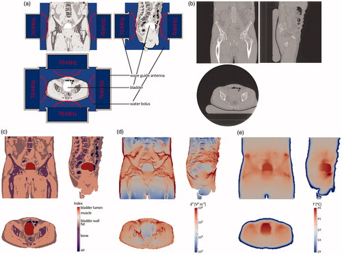
Figure 1. Treatment planning process. First, the patient is treated (a) using four 70 MHz wave guide antennas placed in a ring around the patient. At the end of the treatment session, a CT scan is made (b). This scan is automatically segmented into air, bone, fat, and muscle, and the bladder is delineated by a physician (c). Using this segmentation, the electromagnetic field is computed (d). Finally, the temperature distribution in the patient is computed (e). All images show the coronal view (top right), sagittal view (top left), and axial view (bottom) through the centre of gravity of the scanned patient volume.

In the past decades much progress has been made in the accuracy and reliability of treatment planning [29,30]. A major step forward was the use of more reliable input data. Recent research has shown that the dielectric properties, and in particular the electric conductivity, of urine differ noticeably from the values hitherto used in our treatment planning system; this was shown to have a significant impact on the specific absorption rate (SAR) and temperature distributions in the pelvic area [31].

Realistic modeling of the bladder is important for hyperthermia treatment of bladder cancer. Current hyperthermia treatment planning systems do not model fluid dynamics in the urinary bladder lumen, effectively modeling it as a solid instead of a fluid. A first step towards implementing fluid dynamics was made by Yuan et al. [32], who modeled convective heat transport by a greatly increased effective thermal conduction for the bladder wall. We took this one step further and developed a full fluid dynamics extension [33,34] to our in-house developed hyperthermia treatment planning system, Plan2Heat [35]. Previously, we showed its relevance in a phantom study [36]. Simulations including convective flow modeling showed peak differences of about 1 °C or over 25%, and noticeable (over ±0.25 °C, or ca 10%) temperature differences up to about 1.0–1.5 cm around the bladder compared to the traditional solid modeling, in line with results reported by Yuan et al. [32]. Therefore, physically accurate fluid modeling may not only be relevant for bladder hyperthermia treatments, but also for treatments of nearby organs such as the cervix uteri [37].

The aim of the current study is to evaluate and quantify the benefit of physically correct fluid modeling in NMIBC patients treated with locoregional hyperthermia. To this end, we compared temperatures measured in patients with temperatures predicted by (1) conventional treatment planning with a perfused muscle-like solid bladder, (2) with bladder content properties without and (3) with flow dynamics.

Materials and methods

Treatment and treatment planning

A consecutive cohort of NMIBC patients who received hyperthermia treatment in our institute between March 2009 and November 2011 were studied retrospectively. At the start of treatment, the bladder is emptied and subsequently filled with 40 mg mitomycin C in 50 ml 0.9% saline using a three-way catheter with a balloon for fixation in the bladder. A multi-sensor type T thermocouple (Ella-CS, Hradec Kralove) with 14 sensors 0.5 cm apart, is inserted through the same catheter and measures temperature in the bladder lumen and urethra. The patient is then heated using the AMC-4/8 hyperthermia device for 60–90 min [17]. Initial phase and amplitude settings are based on protocol, and adjusted during treatment based on temperature measurements, patient feedback and operator experience.

Although we aim for a temperature of 37 °C for the chemotherapeutic solution prior to instillation, measurements show that its temperature is frequently 1–2 °C below 37 °C at the start of treatment (cf. Figure 2(a)). Treatment begins with several one-minute power pulses to test different phase-amplitude settings. When the operator has decided on the optimal phase-amplitude settings, the actual treatment begins [27]. After each 25 s, power is switched off for 5 s, during which temperatures are recorded. This power-down time exists to prevent self-heating and electronic disturbance of the thermocouple probes from disturbing the temperature measurements, and to allow the thermocouple to obtain thermal equilibrium with its surroundings [38].

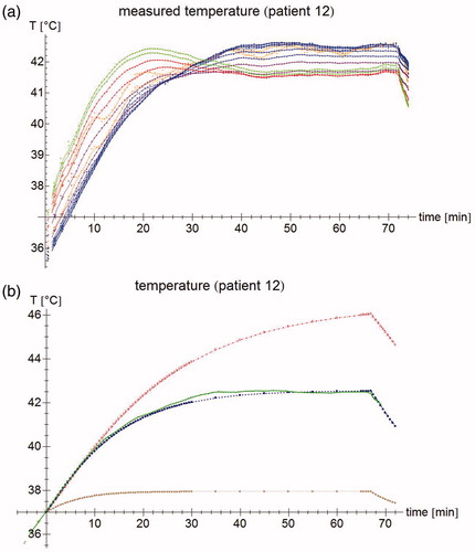
Figure 2. (a) Temperature measurements of patient #12. Each point represents an individual measurement, the lines are moving five-point averages as a guide to the eye. Sensors 1–2 (pressed against the bladder wall) are shown in orange, sensors 3–8 (in the bladder lumen) in blue, sensors 9–10 (fixation balloon) in purple, sensors 11–12 (urethra, near the bladder) in red, and sensors 13–14 (urethra, further from the bladder) in green. While the tip of the probe is inside the bladder, the last few sensors are in the urethra, leading to a different temperature profile. For the first 15 min, the temperature increases roughly linearly; after about 40 min, steady state temperatures are reached. (b) Temperature measurement for sensor #7 (patient #12) at 3 cm from the probe tip (green), and the temperature simulations by the muscle-like model (brown stars), the static model (red empty squares), and the dynamic model (blue filled squares). The time axis for the measurements has been shifted so that T = 37 °C at t = 0 s.

As part of the treatment protocol, a CT scan (GE LightSpeed RT16, resolution 1.0 × 1.0 × 2.5 mm³) was made after one of the hyperthermia treatment sessions (generally the first), with the catheters containing the temperature sensors still in place. A physician delineated the bladder on the CT scan. This scan was used as input for our in-house developed treatment planning system, Plan2Heat [13]. To reduce computation times and meet memory constraints, the image was down-sampled to a 2.5 × 2.5 × 2.5 mm³ cubic grid, in accordance to the current clinical workflow. The scan was automatically segmented based on Hounsfield units into muscle, fat, bone and air regions. The delineated bladder structure was divided into two parts: bladder wall and bladder lumen. The two outermost voxel layers (i.e. 0.5 cm) were assumed to be the bladder wall; this leads to a simulated bladder wall slightly thicker than a typical (healthy) human bladder wall [39,40], but ensures a good quality closed mesh for the bladder wall that does not require manual editing. The remainder of the bladder structure was the bladder lumen, consisting of the instillation fluid and a variable volume of urine. To enhance numerical stability of the fluid simulations, each voxel in the bladder lumen was divided into six pyramids by adding a vertex at the voxel’s centre.

The track of the temperature probe was manually outlined on the same CT. As the individual sensors are not visible on the scan, values at 0.5 cm intervals along these tracks starting from the tip were taken for the comparisons between simulations and measurements. The catheter walls and the fixation balloon were not modeled. At the chosen resolution, and given their poor visibility on the CT scan, the errors introduced by modeling the catheter walls are likely to be greater than the errors of not modeling them. The catheter and the sensors may be assumed to be at thermal equilibrium with their surroundings, given the relatively slow temperature changes involved, and the general absence of sharp temperature gradients, particularly in the bladder [41,42]. The entire process is schematically shown in Figures 1c–e. Only the session after which a CT scan was made, has been analysed.

All regions except the bladder lumen were described by the following six parameters: electric conductivity σ [S m⁻¹], relative permittivity ε_r [–], thermal conductivity k [W m⁻¹ K⁻¹], mass density ρ [kg m⁻³], specific heat per mass C [J kg⁻¹ K⁻¹], and blood perfusion rate ω [kg m⁻³ s⁻¹]. For muscle, the blood perfusion rate at hyperthermic temperatures was used; this means that in areas with a small temperature increase, the temperature is possibly slightly underestimated, but it is correctly estimated in the more relevant areas with a high temperature increase (except for possible small hot spots in areas with an otherwise small temperature rise).

Based on this conductivity and permittivity map, the system solved Maxwell’s equations for the electromagnetic (EM) field, by means of a finite-difference time domain (FDTD) algorithm [44]. For this study, the temperature calculations were performed using a finite element model with explicit time integration, as it simplifies the interaction with the finite element fluid simulations; for the solid regions, cubic elements were used, resulting in a method that is mathematically equivalent to the finite difference method commonly used by Plan2Heat, and confirmed to yield the same results in a previous validation study [34]. In the solid regions, the system computed the temperature distribution based on the electro-magnetic field, using Pennes’ bioheat equation [45]: (1) $$C_{\mathrm{t}}\rho \frac{\partial T}{\partial t}=\nabla \cdot \left(k\hspace{0.17em}\nabla T\right)-\omega C_{\mathrm{b}}\left(T-T_{\text{art}}\right)+Q+P \left[\mathrm{W}\mathrm{ }{\mathrm{m}}^{-3}\right]$$(1)

The left-hand side shows the change in temperature T [K] over time t [s] in the tissue, resulting from the heat sources and sinks on the right-hand side. Here, C_t [J kg⁻¹ K⁻¹] is the tissue’s specific heat per mass and C_b [J kg⁻¹ K⁻¹] the specific heat per mass of blood, while T_art is the arterial blood temperature, fixed at 37 °C and assumed to be the same as the blood temperature in the arterioles and venules. This is also assumed to be the uniform starting temperature. The excess metabolic heat rate Q [W m⁻³] was assumed to be negligible [43]. The last term on the right-hand side is the power absorption P [W m⁻³], which is a function of the electric field $\overrightarrow{E}$ [V m⁻¹]: (2) $$P=\rho \hspace{0.17em}SAR=\frac{1}{2}\sigma E^2\mathrm{ }\left[\mathrm{W}\mathrm{ }{\mathrm{m}}^{-3}\right]$$(2) where SAR [W kg⁻¹] stands for specific absorption rate (SAR) When P = 0 (prior to the start of treatment), the system is in thermal equilibrium, and there are no temperature gradients present in the bladder or its vicinity. There will typically be temperature gradients close to the patient’s skin, due to the surface cooling, but these are generally not relevant for the bladder temperature as they are at a relatively large distance from the bladder.

Fluid modeling

The fluid flow in the bladder lumen was modeled using the Boussinesq approximation to the Navier–Stokes equations, which reads as follows: (3) $$\rho \frac{\partial \overrightarrow{v}}{\partial t}+\rho \nabla \cdot \left(\overrightarrow{v}\overrightarrow{v}\right)=\mu {\nabla }^2\overrightarrow{v}-\nabla p+{\rho }_{\mathrm{k}}\overrightarrow{g}\mathrm{ }\left[\text{kg }{\mathrm{m}}^{-2}\mathrm{ }{\mathrm{s}}^{-2}\right]$$(3)

The left-hand side expresses the co-moving change to velocity $\overrightarrow{v}$ [m s⁻¹] of a fluid element with (constant) mass density ρ [kg m⁻³]. The right-hand side describes the forces acting on the fluid element: the first term is the ‘friction’ between neighbouring fluid elements quantified by the viscosity μ [Pa s], the second the difference in pressure p [Pa]. The third term drives the convection and includes the gravitational acceleration $\overrightarrow{g}$ [m s⁻²], and the (non-constant) kinematic density ρ_k [kg m⁻³], which is assumed to depend linearly on the temperature: (4) $${\rho }_{\mathrm{k}}={\rho }_{\text{ref}}+\beta \left(T-T_{\text{ref}}\right)\mathrm{ }\left[\text{kg }{\mathrm{m}}^{-3}\right]$$(4) where ρ_ref = ρ is the density at the reference temperature T_ref [K] and β [kg m⁻¹ K⁻¹] is the thermal expansion coefficient. We used T_ref = 40 °C (as it is close to the expected temperature range) and β = 3.85 × 10⁻⁴kg m⁻³ K⁻¹ [49].

The equation governing temperature changes in the fluid parts is: (5) $$C_{\mathrm{t}}\rho \frac{\partial T}{\partial t}=k\mathrm{\hspace{0.17em}}{\nabla }^{2}T-C_{\mathrm{t}}\rho \left(\overrightarrow{v}\cdot \nabla T\right)+P\mathrm{ }\left[\mathrm{W}\mathrm{ }{\mathrm{m}}^{-3}\right]$$(5) with all variables as for Equations (1)(1) $$C_{\mathrm{t}}\rho \frac{\partial T}{\partial t}=\nabla \cdot \left(k\hspace{0.17em}\nabla T\right)-\omega C_{\mathrm{b}}\left(T-T_{\text{art}}\right)+Q+P \left[\mathrm{W}\mathrm{ }{\mathrm{m}}^{-3}\right]$$(1) and (3)(3) $$\rho \frac{\partial \overrightarrow{v}}{\partial t}+\rho \nabla \cdot \left(\overrightarrow{v}\overrightarrow{v}\right)=\mu {\nabla }^2\overrightarrow{v}-\nabla p+{\rho }_{\mathrm{k}}\overrightarrow{g}\mathrm{ }\left[\text{kg }{\mathrm{m}}^{-2}\mathrm{ }{\mathrm{s}}^{-2}\right]$$(3) .

The equations were implemented using the open source OpenFOAM toolkit [46]. The boundary conditions on the bladder wall were chosen such that $\overrightarrow{v}$ = 0 on the boundary, and the dynamic pressure gradient was chosen such that the velocity constraint is obeyed by using the standard OpenFOAM pressure boundary condition ‘fixedFluxPressure’. The heat conduction through the boundary was governed by the effective thermal conductivity. The equations were numerically solved using the (transient) PIMPLE algorithm, a combination of the PISO (Pressure Implicit with Splitting of Operator) and SIMPLE (Semi-Implicit Method for Pressure-Linked Equations) algorithms [47]. The reader is referred to Schooneveldt et al. [34] for full details.

At the start of treatment, the temperature is assumed to be homogeneous (so ∇T = 0) and equal to the arterial temperature (so T – T_art = 0). Both Pennes’ equation and the fluid temperature equation then reduce to: (6) $${C_{\mathrm{t}}\rho \frac{\partial T}{\partial t}=P \left[\mathrm{W}\mathrm{ }{\mathrm{m}}^{-3}\right],\text{ or }C}_t\frac{\partial T}{\partial t}=SAR\mathrm{ }\left[\text{kg }{\mathrm{m}}^{-3}\right]$$(6)

Therefore, the initial ∂T/∂t is a measure for the absorbed power, and independent of whether the region is modeled as a solid or as a fluid. Local variations in starting temperature (as may occur in e.g. different organs) may mostly be ignored for the purpose of initial ∂T/∂t measurements, as the initial ∂T/∂t measures only the change in temperature.

At steady state, by contrast, we have ∂T/∂t = 0, and so Pennes’ equation reduces to: (7) $$-k\mathrm{\hspace{0.17em}}{\nabla }^{2}T\mathrm{s}\mathrm{s}+\omega C_{\mathrm{b}}\left(T\mathrm{s}\mathrm{s}-T_{\text{art}}\right)=P\mathrm{ }\left[\mathrm{W}\mathrm{ }{\mathrm{m}}^{-3}\right]$$(7) while the heat equation for the fluid parts is: (8) $$-k\hspace{0.17em}{\nabla }^{2}T\mathrm{s}\mathrm{s}+C_{\mathrm{t}}\rho \left(\overrightarrow{v}\cdot \nabla T\mathrm{s}\mathrm{s}\right)=P\mathrm{ }\left[\mathrm{W}\mathrm{ }{\mathrm{m}}^{-3}\right]$$(8) with Tss the steady state temperature. This means that, from a mathematical point of view, the perfusion heat sink term in the equation is effectively replaced by a term representing heat transport along the fluid flow. This means that heat does not disappear from inside the bladder lumen, but may move between various locations inside the bladder lumen as a result of convection. Heat is only removed from the bladder lumen by thermal conduction to the perfused bladder wall, which is consequently modeled as containing a heat sink. A typical temperature development is shown in Figure 2(a).

In a model with a solid bladder but without perfusion (hereafter called the static model), the heat equation at steady state is simply: (9) $$-k_{\mathrm{t}}{\nabla }^{2}T=P\mathrm{ }\left[\mathrm{W}\mathrm{ }{\mathrm{m}}^{-3}\right]$$(9) which implies that there is no simple (linear) relation between SAR and steady state temperature Tss. In this model as well, there is no heat sink inside the bladder contents, and heat is only removed through conduction to the bladder wall.

Simulations

We performed the following simulations for three different bladder models:

(1) The muscle-like model: we ran the simulation as was customary until now, with the entire bladder wall and lumen modeled as muscle, using the typical muscle parameter values (σ = 0.93 S m⁻¹, ε_r = 75, ρ = 1050 kg m⁻³, C_t = 3639 J kg⁻¹ K⁻¹, k = 0.56 W m⁻¹ K⁻¹), including a blood perfusion term (ω C_b = 12960 J m⁻³ s⁻¹ K⁻¹), and no convective flow modeling. This is part of our current clinical workflow, and is motivated by automatic segmentation algorithms not being able to discriminate between bladder contents and muscle; manual delineation of the bladder is currently not done for other patients than bladder cancer patients.

(2) The static model: we changed the physical and electrical parameters for the bladder lumen hitherto available in the treatment planning system to those of ‘bladder content’ (σ = 1.95 S m⁻¹, ε_r = 78, ρ = 999 kg m⁻³, C_t = 4181 J kg⁻¹ K⁻¹, k = 0.64 W m⁻¹ K⁻¹), and set the blood perfusion rate to zero (ω C_b = 0 J m⁻³ s⁻¹ K⁻¹). In effect, we changed everything from ‘muscle’ to ‘bladder content’, except that we still modeled it as a solid, without fluid dynamics in the bladder lumen.

(3) The convective or dynamic model: we applied the same parameters as in the static model, combined with the flow dynamics, thus yielding a physically more realistic model.

All parameter values are based on literature values; a summary of the different parameters, including references, is given in Table 1. The dielectric values for bladder contents are the average of physiological saline (0.9% NaCl), which is instilled in the bladder, and urine, which naturally accumulates in the bladder during treatment. In all simulations, the clinically applied amplitude and phase settings obtained from the treatment log file were used.

Table 1. parameter values for the three different simulations performed for each patient. Parameters are obtained from: Balidemaj et al. [51], Gabriel and Gabriel [53–54], Rossmann and Haemmerich [55], Klein and Swift [56] and Sharqawy et al. [57].

Bladder modeled as	σ [S m^–1]	εr [–]	ρ [kg m^–3]	Ct [J kg^–1 K^–1]	k [W m^–1 K^–1]	ω Cb [J m^–3 s^–1 K^–1]	Flow
Muscle	0.93	75	1050	3639	0.56	12960	No
Static urine	1.95	78	999	4181	0.64	0	No
Dynamic urine	1.95	78	999	4181	0.64	0	Yes

Analysis

The analysis can be divided into two parts: the first part concerns SAR and the rate of temperature change in the fluid and bladder wall during the initial heating-up phase, the second part concerns the steady state temperature. For each part, the models are compared with the measurements. In addition to the results on the group level, we show full details for a single (representative) patient, whose treatment proceeded without any phase-amplitude adjustments, or technical or clinical complications. Although agreement with measurements is the most relevant aspect for clinical use, a comparison between the models does add some additional insights. Most importantly, it is possible to compare the entire bladder volume, the bladder wall and the bladder surface in a precise manner, whereas measurements are only available for a limited number of points. We computed hyperthermia temperature volume histograms for the bladder wall, the bladder lumen and the interface between the two, representing the urothelial layer. The comparison of the muscle-like model with the dynamic model shows the full effect of moving from the original to the new procedure; the comparison of the static with the dynamic model singles out the effect of modeling fluid dynamics.

In addition, we determined for each patient the bladder volume at the end of treatment, and the population average bladder volume (μ_V) and bladder volume standard deviation (σ_V).

Initial temperature rise

We analysed the accuracy of the SAR predicted by each model. Whereas the SAR can be directly determined for the simulations—indeed, it is the input for the temperature computations—it is practically impossible to measure during treatment. However, as was shown in Equation (6)(6) $${C_{\mathrm{t}}\rho \frac{\partial T}{\partial t}=P \left[\mathrm{W}\mathrm{ }{\mathrm{m}}^{-3}\right],\text{ or }C}_t\frac{\partial T}{\partial t}=SAR\mathrm{ }\left[\text{kg }{\mathrm{m}}^{-3}\right]$$(6) , under the assumption of a homogeneous starting temperature, the initial rate of temperature increase is proportional to the SAR and this initial temperature rise is measurable. The start of treatment was taken as reference point.

There is a large inter- and intra-patient variation in both modeled and measured temperature rise. In order to perform a meaningful comparison, we calculated the normalized SAR (SAR_norm) by: (10) $${\text{SAR}}_{\text{norm}}=10\mathrm{ }{\log }_{10}\mathrm{ }\left(\frac{{\mathrm{\Delta }T}_{\text{modelled}}}{{\mathrm{\Delta }T}_{\text{measured}}}\right)\mathrm{ }\left[\mathrm{d}\mathrm{B}\right],\text{ at }t\mathrm{ }=\mathrm{ }0.$$(10)

A SAR_norm of zero means that the simulated SAR is equal to the measured SAR, whereas a positive SAR_norm implies an overestimation of the actual SAR, and a negative SAR_norm an underestimation. It should be taken into account, however, that some uncertainty in ${\mathrm{\Delta }T}_{\text{modelled}}$ is to be expected as the initial state as modeled assumes an equilibrium in which the entire body is at 37 °C, including the bladder contents. As the bladder is filled with a chemotherapeutical instillation just prior to the start of the hyperthermia session, some deviations from this assumption may be expected.

As convective heat transport and perfusion, respectively, are initially negligible, as indicated in Equation (6)(6) $${C_{\mathrm{t}}\rho \frac{\partial T}{\partial t}=P \left[\mathrm{W}\mathrm{ }{\mathrm{m}}^{-3}\right],\text{ or }C}_t\frac{\partial T}{\partial t}=SAR\mathrm{ }\left[\text{kg }{\mathrm{m}}^{-3}\right]$$(6) , we can expect to find identical results for the static and dynamic urine models during the first phase of heating up. The difference between the two provides some insight in the quality of the approximation that SAR = C_t ΔT/Δt, where, clinically, Δt is typically 30 or 60 s; comparison with the computed SAR yields further information on how well SAR is approximated by initial temperature rise. Clinically, the temperature rise over the first 30 or 60 s is generally taken to be a measure of SAR, ignoring the effects of conduction, perfusion and (for the bladder contents) convection, but these effects may in fact not be negligible in every region. As the steady state temperature depends primarily on the absorbed power, it is important to estimate the accuracy of the computed SAR, to discriminate between the effect of errors in SAR and other sources of error in the steady state temperature computations.

Combining Equation (6)(6) $${C_{\mathrm{t}}\rho \frac{\partial T}{\partial t}=P \left[\mathrm{W}\mathrm{ }{\mathrm{m}}^{-3}\right],\text{ or }C}_t\frac{\partial T}{\partial t}=SAR\mathrm{ }\left[\text{kg }{\mathrm{m}}^{-3}\right]$$(6) with Equations (7)(7) $$-k\mathrm{\hspace{0.17em}}{\nabla }^{2}T\mathrm{s}\mathrm{s}+\omega C_{\mathrm{b}}\left(T\mathrm{s}\mathrm{s}-T_{\text{art}}\right)=P\mathrm{ }\left[\mathrm{W}\mathrm{ }{\mathrm{m}}^{-3}\right]$$(7) and (8)(8) $$-k\hspace{0.17em}{\nabla }^{2}T\mathrm{s}\mathrm{s}+C_{\mathrm{t}}\rho \left(\overrightarrow{v}\cdot \nabla T\mathrm{s}\mathrm{s}\right)=P\mathrm{ }\left[\mathrm{W}\mathrm{ }{\mathrm{m}}^{-3}\right]$$(8) , respectively, and evaluating at steady state, we get: (11) $$-k\mathrm{\hspace{0.17em}}{\nabla }^{2}T\mathrm{s}\mathrm{s}+\omega C_{\mathrm{b}}\left(T\mathrm{s}\mathrm{s}-T_{\text{art}}\right)=C_{\mathrm{t}}\rho \frac{\partial T\left(0\right)}{\partial t}\approx C_{\mathrm{t}}\rho \frac{\Delta T_{\text{initial}}}{\Delta t}\mathrm{ }\left[\mathrm{W}\mathrm{ }{\mathrm{m}}^{-3}\right]$$(11)

and (12) $$-k\mathrm{\hspace{0.17em}}{\nabla }^{2}T\mathrm{s}\mathrm{s}+C_{\mathrm{t}}\rho \left(\overrightarrow{v}\cdot \nabla T\mathrm{s}\mathrm{s}\right)=C_{\mathrm{t}}\rho \frac{\partial T\left(0\right)}{\partial t}\approx C_{\mathrm{t}}\rho \frac{\Delta T_{\text{initial}}}{\Delta t}\mathrm{ }\left[\mathrm{W}\mathrm{ }{\mathrm{m}}^{-3}\right]$$(12) relating the steady state temperature to the initial temperature rise for the two different models. These equations show that for the same initial temperature rise, the steady state temperature can exhibit very different behavior; therefore, very distinctive correlations between (measurable) initial temperature rise and (measurable) steady state temperature are to be expected which may be used to discriminate between the models.

Steady state temperature

Moving to the steady state phase represented by Equations (11)(11) $$-k\mathrm{\hspace{0.17em}}{\nabla }^{2}T\mathrm{s}\mathrm{s}+\omega C_{\mathrm{b}}\left(T\mathrm{s}\mathrm{s}-T_{\text{art}}\right)=C_{\mathrm{t}}\rho \frac{\partial T\left(0\right)}{\partial t}\approx C_{\mathrm{t}}\rho \frac{\Delta T_{\text{initial}}}{\Delta t}\mathrm{ }\left[\mathrm{W}\mathrm{ }{\mathrm{m}}^{-3}\right]$$(11) and (12)(12) $$-k\mathrm{\hspace{0.17em}}{\nabla }^{2}T\mathrm{s}\mathrm{s}+C_{\mathrm{t}}\rho \left(\overrightarrow{v}\cdot \nabla T\mathrm{s}\mathrm{s}\right)=C_{\mathrm{t}}\rho \frac{\partial T\left(0\right)}{\partial t}\approx C_{\mathrm{t}}\rho \frac{\Delta T_{\text{initial}}}{\Delta t}\mathrm{ }\left[\mathrm{W}\mathrm{ }{\mathrm{m}}^{-3}\right]$$(12) , we subsequently computed the normalized steady state temperature rise ΔTss_norm, where the steady state temperature Tss was assumed to be the average temperature of the last 90 s prior to the end of treatment: (13) $${\mathrm{\Delta }T\mathrm{s}\mathrm{s}}_{\text{norm}}=10\mathrm{ }{\text{log}}_{10}\left(\frac{{T\mathrm{s}\mathrm{s}}_{\text{modelled}}-37\hspace{0.17em}°\mathrm{C}}{{T\mathrm{s}\mathrm{s}}_{\text{measured}}-37\hspace{0.17em}°\mathrm{C}}\right)\mathrm{ }\left[\mathrm{d}\mathrm{B}\right].$$(13)

To determine whether Pennes’ equation is a good approximation for the modelled tissue, we compared ΔTss_norm to SAR_norm. Tss is expected to be strongly (linearly) correlated to SAR for the muscle-like model as the contribution of thermal conduction is relatively small compared to the perfusion term (at least in the target area at some distance from the cooled skin, and apart from an occasional hot spot). A weak or non-linear correlation will imply that Pennes’ equation is not a good approximation for the modelled tissue (in casu the bladder contents). For both the static and the dynamic models, there is no reason to expect a strong linear correlation between local SAR and local steady state temperature.

From a clinical point of view, however, the most relevant quantity is the absolute steady state temperature error ΔTss = T_modeled – T_measured. This quantity was determined per measurement location and averaged over the entire probe length, the latter to reduce the effect of random or very local errors. The error in (estimated) T₅₀ is reported separately. In general, T_n is defined as the temperature such that n% of the volume has a temperature equal to or higher than T_n, so T₅₀ is equivalent to the median temperature. As we are here concerned with the steady state temperature, temperature quantiles are interpreted solely as spatial quantiles, not temporal quantiles.

Results

In the inclusion period, 18 patients were treated for NMIBC, 14 of which could be analysed for the present study. The measured temperatures during clinical treatment are compared to the temperatures simulated by three models (muscle-like, static urine and dynamic urine). We show the data on the temperature rise during initial heating and the steady state temperature at the end of treatment for the entire group. In addition, temperature profiles are shown for a typical patient, patient #12, in Figure 2. For this patient, there were no changes in phase or amplitude settings during treatment. Moreover, this patient had a slightly above average bladder lumen at the end of treatment (bladder volume V = 211 ml, population mean volume µ_V = 177 ml, population standard deviation σ_V = 65 ml; as determined by counting voxels in the segmented model), so any effects are likely to be clearly visible while still being representative. We will first focus on the initial temperature rise or SAR, then on the steady state temperature, and subsequently on the correlation between these two quantities.

Initial temperature rise

Figure 2(a) shows the temperature measurements in the bladder during a typical bladder treatment. The first 10–20 min, the temperature rises sharply, and after another 15–30 min transition period, the temperature becomes fairly stable within ∼0.2 °C. Measurements that are close to the catheter balloon may exhibit a slightly aberrant behavior. Figure 2(b) shows the same measurement for ‘central’ sensor #7, located 3 cm from the tip of the probe (inside the liquid bladder contents and not touching the bladder wall) and the simulated temperature at the same location.

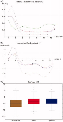
The initial temperature rise is related to SAR, as explained in Equation (6)(6) $${C_{\mathrm{t}}\rho \frac{\partial T}{\partial t}=P \left[\mathrm{W}\mathrm{ }{\mathrm{m}}^{-3}\right],\text{ or }C}_t\frac{\partial T}{\partial t}=SAR\mathrm{ }\left[\text{kg }{\mathrm{m}}^{-3}\right]$$(6) . Figure 3(a) shows the measured and simulated temperature rise after 30 s along the measurement probe. As this value differs strongly between patients, we also looked at SAR_norm, shown in Figure 3(b). Note that SAR_norm is defined as the logarithm of the relative temperature rise and is therefore a measure of temperature, rather than a measure of power. In this patient, the dynamic and static models are much closer to zero than the muscle-like model, and they therefore perform better. As the ΔT measurement gives only an approximation of the true SAR, we included both the simulated SAR and the resulting simulated temperature rise in our analyses. Figure 3(c) shows the aggregated results for all patients in a box plot, showing median, inter-quartile range, minimum, and maximum values.

Figure 3. (a) Temperature rise per sensor for patient #12 after 30 s. Green filled circles: measurements, brown stars: muscle-like model, red empty squares: static model, blue filled squares: dynamic model, purple empty circles: expected temperature rise based only on computed specific absorption rate (SAR). (b) Normalized SAR per sensor after 30 s. Brown stars: muscle-like model, red empty squares: static model, blue filled squares: dynamic model. (c) Aggregated normalized SAR, showing median, inter-quartile range, minimum and maximum, and outliers.

For one patient (patient #15), the mean SAR_norm could not be computed because of technical complications at the start of treatment, leading to fluctuating temperatures, so this patient was excluded for the mean SAR_norm computations. For the muscle-like model, mean SAR_norm per patient was −3.4 dB averaged over all patients (range –9.6 through −0.22 dB), that is, simulated SAR was on average 45% of the measured SAR (range 11–95%). For the static and dynamic models, this was −1.78 dB (ranges −7.4 through 0.5 dB, and −7.0 through 0.4 dB, respectively), or 66% (18–112% and 20–108%). As the computed SAR is identical, the small difference shows the equally small effect of perfusion versus convection at start of treatment. It should be kept in mind that this difference will increase with the measurement interval Δt, so the small difference indicates that the interpretation of ΔT is robust for the clinically used time intervals of 30 or 60 s.

In 8 out of 14 patients, the muscle-like model has a lower simulated SAR for the urine (mean 15.1 W kg⁻¹, median 9.4 W kg⁻¹) compared to the static and dynamic models (mean 17.7 W kg⁻¹, median 16.1 W kg⁻¹), due to the much lower electric conductivity of muscle tissue compared to urine, as shown in Table 1. Combined with the blood perfusion in the muscle-like model, this leads to generally very low urine and tumor temperatures, even though bladder wall SAR is typically (in 10/14 patients) slightly higher in the muscle-like model (mean 22.4 W kg⁻¹, median 19.13 W kg⁻¹) compared to the static and dynamic models (mean 20.0 W kg⁻¹, median 16.9 W kg⁻¹).

The muscle-like model, using the dielectric values for muscle instead of urine, tends to underestimate the SAR in the bladder: on average, the predicted SAR is less than half of the measured SAR. Using bladder content instead of muscle values for σ and ε gives a better, but still too low SAR approximation (about two thirds of the measured SAR). This is likely partly due to the inter-patient variability in σ, which is not taken into account. In addition, a systematic error is induced by the gradual increase in bladder lumen between the time of initial temperature rise measurement, and CT imaging; however, we found no correlation between bladder volume on the CT and SAR_norm value (data not shown). A further error is introduced by the uncertainties in patient anatomy outside the bladder, which influence both the loco-regional electromagnetic field, and the overall power absorption, through normalizing the absorbed power to the delivered power.

Steady state temperature

The correlation between measured and computed ΔT_initial and Tss is plotted in Figure 4(a). This figure shows that the measured steady state temperature is weakly correlated to the measured SAR (adjusted R² = 0.41), whereas the muscle-like model shows a very strong correlation, as expected (adjusted R² = 0.91). The static and dynamic models show (virtually) no correlation (adjusted R² equals 0.00 and 0.12, respectively). The low R² for the static model can be explained by the fact that the (modeled) SAR is fairly homogeneous within the bladder contents, due to the relatively high σ, whereas the Tss depends mostly on the distance to the bladder wall, the only heat removal mechanism being thermal conduction to the perfused bladder wall. The low R² for the dynamic model will be the result of convective mixing. The R² for the measurements is relatively high compared to R² for the static and dynamic models. This is mostly caused by the inter-patient effect that in patients with a relatively high SAR, also higher steady state temperatures are obtained. The difference between the measurements and the dynamic model appear for large part to be caused by a wider spread in the predicted temperatures for a given SAR, compared to the spread in the measured temperatures.

Figure 4. (a) Correlation between initial temperature rise at t = 30 s and steady state temperature. Lines show best linear fit. (b) Correlation between normalized SAR and normalized steady state temperature. A strong correlation means that errors in predicted steady state temperature are largely explained by errors in SAR computation. (c) Residual plots of the correlation, showing a clear bias on a per patient basis, but a good distribution for the group. Dashed lines separate points belonging to different patients. (d) Correlation for patient #12, showing that correlation parameters within one patient are radically different form the group ones.

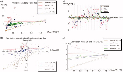
Figure 4(b) shows the correlation between normalized SAR and normalized Tss for the three models. The muscle-like model generally predicts too low temperatures (points beneath the x-axis); the static model generally too high, and the dynamic model falls in between. Temperature errors in the muscle-like model are fairly strongly correlated to errors in SAR (adjusted R² = 0.77). Temperature errors in static and dynamic models are not explained by errors in SAR (adjusted R² equals 0.00 and 0.12, respectively). The residuals of the correlation are defined as the difference between the actually ‘observed’ (measured or modeled) value, and the value estimated by the correlation. The residuals represent the random noise, if the studied phenomenon is fully explained by the modeled variables. If the residuals clearly deviate from a Gaussian distribution, it generally implies there are other relevant variables that are unaccounted for. The residuals of the correlation between absolute SAR and ΔTss in Figure 4(c) show that the correlation does not hold within an individual patient, as generally the residuals are clearly not randomly distributed around zero, but often appear to follow a curve. Additionally, the residuals for a certain model tend to have the same sign within one patient, implying that within a single patient, the steady state temperature for all measurement points is higher or lower than expected based on the initial temperature rise and the average overall correlation. For instance, Figure 4(d) shows that for patient #12 the measured correlation between SAR and ΔTss is very weakly negative (with adjusted R² = 0.02), whereas the correlation over all patients is positive. This is in clear contrast with the muscle-like model, which has an excellent correlation with adjusted R² = 0.98, confirming that Pennes’ model does not hold in the bladder lumen.

These three models result in strikingly different temperature profiles within the bladder. Figure 5 shows typical temperature profiles for the different models. The muscle-like model predicts a low and fairly uniform temperature distribution in the bladder, with temperatures that increase toward the bladder wall. The static model, on the other hand, shows a temperature that increases towards the middle point of the bladder, and locally reaches very high temperatures (>50 °C, for patient #12). The dynamic model, by contrast, predicts a rather uniform temperature distribution within the bladder lumen, and a temperature that is only slightly higher than the bladder wall temperature.

Figure 5. Modeled temperature profiles through the patient in the x-, y-, and z-directions. The vertical lines indicate the outer edge of the bladder lumen (yellow) and the bladder wall (purple), respectively.

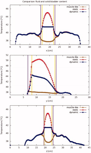
The predicted temperature in the bladder wall (treatment target) is more homogeneous in the dynamic case than in the static case. Since temperatures predicted by the muscle-like model are so much lower, there is more homogeneity than in the dynamic case; this is shown in Figure 6. Figure 6(a) shows the absolute standard deviation, while Figure 6(b) shows the standard deviation divided by the mean temperature rise, or relative standard deviation. Figure 7 shows the temperature volume histogram for the bladder wall, the bladder lumen, and the interface between the two (modeling the urothelial layer), showing that the predicted median temperature is highest for the dynamic model. Table 2 shows the aggregated data for all patients.

Figure 6. Modeled temperature standard deviation (a: absolute, and b: relative) per patient for the bladder contents and the bladder wall.

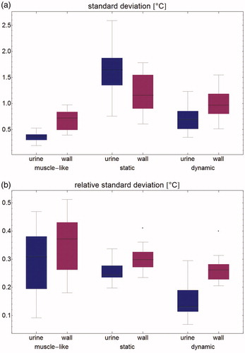
Figure 7. Temperature volume histogram, showing the modeled steady state temperature distribution for the bladder contents (dotted), the bladder wall (solid), and the interface between those two regions, representing the urothelium (dashed); each as computed by the muscle-like model (brown), the static model (red) and the dynamic model (blue).

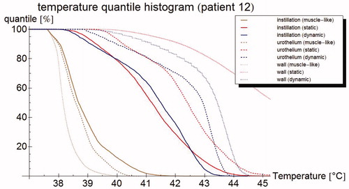
Table 2. Mean temperature in °C for all patients (mean, standard deviation, and minimum and maximum temperature are given) for the three different simulations of the bladder lumen: 'muscle-like' models the bladder lumen as solid, perfused muscle; ’static urine' uses physical parameters for urine, but no flow dynamics; and 'dynamic urine' also applies flow dynamics.

	Muscle-like		Static urine		Dynamic urine
	Mean ± SD [°C]	Range [°C]	Mean ± SD [°C]	Range [°C]	Mean ± SD [°C]	Range [°C]
Urine	38.52 ± 0.36	37.86–40.75	44.00 ± 1.84	39.10–47.75	41.63 ± 0.65	38.85–42.67
Wall	38.97 ± 0.67	37.68–42.57	40.86 ± 1.14	38.10–45.33	40.50 ± 0.92	38.01–43.87

Finally, the clinically most relevant aspect is how well the model predicts the temperatures in tissue during treatment, and for this the absolute temperature error is the most relevant quantity. Figure 8(a) shows the absolute and normalized steady state temperature profile for patient #12 along the measurement probe with the simulated temperatures. Figure 8(c) and (d) show box plots of all sensors for all patients combined for Tss_norm and the error in T₅₀; the errors are smallest for the dynamic model by a clear margin. The results per patient and for the whole group are also shown in Table 3. The muscle-like model always performs worst. For 2 out of 14 patients, the static model performs best, for the other 12 the dynamic model is equal or superior to the static model. Overall, the dynamic model is the best performing model, with the lowest mean error, lowest root mean square error, and lowest average difference in median temperature or T₅₀; that last parameter, in particular, is reduced from 3.8 °C for the muscle-like model, to 0.6 °C for the dynamic model.

Figure 8. (a) Steady state temperature per sensor as measured (filled circles), and as predicted by the muscle-like model (stars), the static model (empty squares) and the dynamic model (filled squares). The measured temperatures and those predicted by the dynamic model are relatively homogeneous and close to each other, whereas the muscle-like model grossly underestimates the steady state temperature, and the static model overestimates the same. (b) Aggregated normalised steady state temperature Tss for all patients. The muscle-like model (brown, left) predicts temperatures that are generally far too low, the static model (red, middle) tends to overestimate the temperature and has a wide spread in temperature errors, and the dynamic model (blue, right) tends to underestimate the temperature, and has a much smaller spread in temperature errors. (c) Error in T₅₀ for the muscle-like (brown, right), static (red, middle), and dynamic (blue, right) models. Although the dynamic model tends to underestimate temperatures, it has by far the smallest errors of the three models.

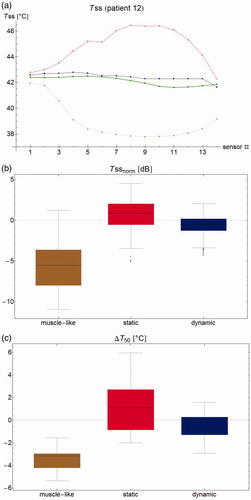
Table 3. Performance of the muscle-like, static and dynamic models on a per patient basis, determined by the difference between measured and modeled temperatures and the sensor locations.

	Muscle-like			Static urine			Dynamic urine
	µ ± σ	RMS	ΔT50	µ ± σ	RMS	ΔT50	µ ± σ	RMS	ΔT50
1	–4.22 ± 0.62	4.26	–4.40	0.76 ± 0.73	1.04	0.78	–0.96 ± 0.36	1.02	–0.99
2	–3.23 ± 1.40	3.50	–3.79	–0.86 ± 1.21	1.45	–1.20	–1.63 ± 1.49	2.17	–2.15
3	–1.55 ± 0.42	1.60	–1.63	–1.25 ± 0.40	1.31	–1.32	–1.29 ± 0.41	1.35	–1.32
5	–3.33 ± 0.46	3.36	–3.41	0.60 ± 1.19	1.29	0.77	–0.75 ± 0.35	0.82	–0.69
6	–2.84 ± 0.55	2.89	–3.01	1.44 ± 1.72	2.20	1.64	–0.24 ± 0.52	0.56	–0.07
7	–2.94 ± 0.67	3.01	–3.12	1.50 ± 1.06	1.81	1.80	0.37 ± 1.19	1.21	0.59
8	–2.79 ± 1.04	2.97	–3.33	4.80 ± 0.30	4.81	4.84	0.29 ± 0.26	0.38	0.16
9	–3.12 ± 0.45	3.15	–3.30	5.95 ± 3.40	6.79	6.94	1.57 ± 0.49	1.64	1.77
11	–4.42 ± 0.29	4.43	–4.60	2.72 ± 1.03	2.89	2.97	–0.28 ± 0.34	0.43	–0.38
12	–3.19 ± 1.33	3.43	–3.95	2.87 ± 1.69	3.30	2.96	0.33 ± 0.24	0.41	0.25
13	–4.87 ± 0.68	4.92	–4.98	2.99 ± 0.59	3.04	3.45	–0.63 ± 0.47	0.78	–0.43
15	–3.14 ± 0.54	3.19	–3.23	–1.03 ± 1.47	1.75	–1.10	–1.70 ± 1.01	1.96	–1.48
16	–3.55 ± 1.50	3.84	–4.20	0.39 ± 0.91	0.97	0.34	–0.80 ± 0.90	1.18	–0.89
18	–5.36 ± 0.62	5.39	–5.44	–1.99 ± 1.38	2.40	–1.79	–2.92 ± 0.36	2.94	–2.70
avg	–3.5 ± 1.0	3.6	–3.7	1.3 ± 2.4	2.5	1.5	–0.6 ± 1.2	1.2	–0.6
corr.	–2.0 ± 1.4	2.9	–2.6	1.4 ± 1.8	3.6	1.6	–0.3 ± 0.8	1.6	–0.2

Per model, the mean error (µ) and standard deviation (σ), the root mean square error (RMS), and the error in median temperature (ΔT₅₀) are given.

Model performance is indicated with three shades of green, a darker shade indicates better performance (light: ΔT < 0.5 °C, medium: 0.5 < ΔT < 1.0, dark: 1.0 < ΔT < 2.0; for the RMS, the thresholds are multiplied by √2).

The last row shows the average values after correcting for low SAR using the best fit shown in Figure 4a and a correction factor for the SAR of 1/0.45 for the muscle-like model and 1/0.66 for the static and dynamic models.

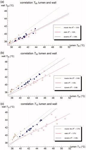
The urine and bladder wall temperature parameters are well correlated for all models: adjusted R² > 0.7 for all T_n, with 0 < n < 100 for the muscle-like and dynamic models, and for 2 < n < 100 for the static model. This correlation is particularly strong for the dynamic model (adjusted R² > 0.95 for T_n, with 3 < n < 74, and for 6 < n < 50, adjusted R² > 0.98), as is also shown in Figure 9. This means that based on measurements in the bladder lumen, the bladder wall thermal parameters like T₁₀, T₅₀, and T₉₀ can be determined with good accuracy, and especially the bladder wall T₅₀ with excellent accuracy.

Figure 9. Correlation of the (measurable) urine temperature and (clinically relevant) wall temperature for the T₉₀ (a), T₅₀ (b) and T₁₀ (c), respectively, according to the muscle-like model (brown star), the static model (red empty squares), and the dynamic model (blue filled squares). The lines show the best linear fit, based on least squares.

The Grashof number was computed to be 3.2 ± 1.5 × 10⁵ (mean ± SD), and the Rayleigh number was 1.5 ± 0.72 × 10⁶ (mean ± SD). These confirm that temperature induced convection plays a significant role and show that the flow can safely be assumed to be non-turbulent.

Discussion

This article adds a new step to the work reported by Yuan et al. [32]. At this time, this is the only publication the authors are aware of that discusses a similar study, applying locoregional hyperthermia to the bladder using the BSD-2000 system: a comparable hyperthermia device, with a comparable heating pattern [48]. Whereas they made a first effort to take fluid behavior in the bladder into account using a highly increased effective thermal conductivity, we have actually modeled the fluid flow. As a result, our predicted error in median temperature is much smaller (0.6 °C) than the error reported by Yuan et al. [32] (1.3 °C). A strong point of the Yuan et al. [32] study is that they measure the dielectric properties of the bladder lumen after treatment, which should improve the quality of retrospective analyses. The values used in our simulations, by contrast, were based on literature values.

Still, the higher electric conductivity of urine compared to muscle leads to a higher power absorption in the urine. As the urine itself is not perfused, heat removal is limited to heat conduction to the bladder wall, which means that heat removal is slower than it would be for perfused muscle. Combined, these effects lead to a substantially higher temperature in the bladder when parameter values valid for urine are used, compared to using the values for perfused muscle.

An error in the calculated SAR will generally result in a similar error in calculated Tss, aside from small, local anomalies. This is particularly evident for the muscle-like model, where a clear correlation between SAR and Tss is expected, as was explained following Equation (8)(8) $$-k\hspace{0.17em}{\nabla }^{2}T\mathrm{s}\mathrm{s}+C_{\mathrm{t}}\rho \left(\overrightarrow{v}\cdot \nabla T\mathrm{s}\mathrm{s}\right)=P\mathrm{ }\left[\mathrm{W}\mathrm{ }{\mathrm{m}}^{-3}\right]$$(8) . This was the case for the muscle-like model, but to a much smaller extent also for the static and dynamic models. While the measured SAR is weakly correlated to the measured steady state temperature in the aggregate data, this correlation completely disappears in a per patient analysis. This implies that while the mean or median temperature may be somewhat accurately estimated based on SAR, local variations in temperature are not explained by variations in SAR. This also implies that using Pennes’ bioheat equation for liquid bladder contents does not yield an adequate approximation of heat transport in and around the liquid filled urinary bladder.

We found that the predicted initial temperature rise for the muscle-like model is only about 45% of the measured temperature rise, and about 66% for the static and dynamic models. If we simply correct the computed SAR for this amount, by increasing the simulated temperatures with the best fit formula for the correlation between initial temperature rise and steady state temperature (plotted in Figure 4(a)), and recalculate the quantities in Table 3, we find the 'corrected' quantities which are averaged in the last row of Table 3. This suggest that improving our SAR computations might reduce the error in predicted steady state temperature for the muscle-like and dynamic models; in particular, the mean error for the dynamic model would reduce to 0.3 °C, and the error in T₅₀ to 0.2 °C, which is of the same magnitude as the fluctuations in steady state temperature occurring during treatment.

The static model has no heat removal mechanism in the bladder content, apart from (relatively inefficient) heat conduction to the bladder wall, and therefore predicts very high temperatures in the urine. Modeled temperatures in the bladder wall are only slightly higher than in the dynamic case, showing that heat removal in the bladder wall and/or heat transport through the bladder wall is very efficient.

The muscle-like model has a relatively low SAR, leading to low temperatures in the bladder lumen. Combined with the high blood perfusion (remember that in the muscle-like model, the lumen is modeled as if it were a muscle), this results in a low and fairly uniform temperature distribution in the bladder lumen, with temperatures that increase towards the bladder wall. The static model, on the other hand, shows a temperature that increases towards the center of the bladder, and reaches unrealistically high maximum temperatures, because of a relatively high SAR, and the absence of an effective heat removal mechanism: there is only heat conduction to the perfused bladder wall. The dynamic model, by contrast, has a very efficient convective heat transport, leading to a rather uniform temperature distribution within the bladder lumen, that is very well correlated to the bladder wall temperature.

The very strong correlation between the computed temperature parameters (e.g. T₁₀, T₅₀ and T₉₀) of the bladder lumen and those of the bladder wall, implies that measurements made in the lumen can be used to determine these parameters for the wall with great confidence. Of these parameters, Franckena et al. [8] found that the median temperature gives the best dose-effect relationship for cervix tumors treated with radiotherapy and hyperthermia, although dose-effect relationships have not yet been determined for bladder cancer treated with hyperthermia and radiotherapy or chemotherapy. The correlation is less reliable for T_max, clinically relevant for preventing toxicity, but due to the limited number of measurement points, T_max cannot be accurately determined in any case, not even when measured at the bladder wall itself. As the bladder wall temperature is generally lower than the fluid temperature, though—at least when using external microwave applicators—, an upper limit for T_max can be estimated with reasonable confidence. Nevertheless, patient feedback remains important to prevent potential overheating. The dynamic model in particular is also somewhat less strongly correlated for T_n with n > 75, which is not surprising, as the cooler parts of the bladder wall will be those farthest away from the bladder lumen.

There are factors associated with the input data that might have influenced the quality of the planning for all three models. The CT scan is made following the hyperthermia treatment session, which lasts about 90 min. This means the amount of bladder lumen that is visible on the CT scan, and which is used for all calculations, represents the maximum amount present during the treatment. Therefore, the effect size reported in this article is likely to be the maximum effect size during treatment. Moreover, the real patients' anatomy (including variations over time in tissue properties like perfusion) are less static than the CT-scan based reconstructions suggest, as can be seen from the fact that the steady state temperature tends to vary a little over time (typically a few tenths °C), whereas it is practically constant for the simulations. These changes have different time scales. Filling of the bladder is essentially a monotonously increasing phenomenon, and changes in dielectric values of the bladder lumen due to its changing composition can also be assumed to be slow, whereas bowel motions and changes in blood flow in the heated area have a much shorter timescale. This means that the latter will probably average out over a large enough time period of the treatment, but may have a stronger influence on predictions at a specific point in time. Emptying of the bladder may also occasionally occur, but this is of course highly undesirable in the case of chemotherapeutic instillations. Other factors affecting tissue temperatures on longer time scales are whole body thermoregulation, especially important when heating extended body regions for a prolonged period of time, and slow internal organ sliding resulting from the posture change when the patient lies down for a long time.

Because of these changes in anatomy during treatment and inherent uncertainties in tissue properties, as well as limitations in number of distinguished tissues and the simplified thermal model neglecting for instance the impact of individual (large) vessels or the difference between arterial and venous temperature, there is some uncertainty in the simulated temperature distributions. Additionally, the modeling resolution in this study was chosen in accordance to our present clinical workflow, yielding practical simulation times. Simulation of phantom experiments (unpublished data) indicated that convergence is obtained at the chosen resolution. More extensive resolution/convergence studies including realistic patient anatomies might be desirable, but are highly computationally demanding. However, while these errors may vary greatly between patients, they will be the same when different bladder models for the same patient are being compared. The effect size found will therefore be relatively insensitive to these uncertainties.

Another source of uncertainty is due to difficulties in discerning the temperature probe on some of the scans. Comparison between measured and simulated temperatures may actually be comparing temperatures at (somewhat) different locations. However, given the bladder lumen’s fairly homogeneous temperature distribution, the errors within the bladder are expected to be similarly small. This is different for sensors that are not fully within the bladder lumen, but for example pressed against the bladder wall, inside an air pocket, or simply outside the bladder; here these errors can be more pronounced.

Phase and/or amplitude settings are often adjusted during treatment, which was not taken into account in our analysis. When the planning software is coupled to the actual treatment monitoring system, like the clinical version of Plan2Heat, these adjustments will be taken into account automatically, hopefully improving reliability of the simulation results even further. Nevertheless, there can be noticeable fluctuations in the temperature, even when phase and amplitude are stable: although typical fluctuations in steady state are roughly 0.2 °C, spikes exceeding 1 °C may occur (in some cases due to the patient losing urine during treatment or bladder spasms), and some patients never reach a steady state at all. These fluctuations are due to changes in patients anatomy during treatment (for instance, bowel motion and moving bowel gas), and also changes in dielectric properties of the bladder lumen, as the mitomycin C instillation is mixed with urine. These changes are not reflected in the present simulations, which predict a very stable steady state.

As the current software cannot yet be used for treatment optimization, due to the long computation times (roughly 15 s of computation time on a typical desktop PC to simulate 1 s of treatment time), an intermediate step may include optimizing phase and amplitude settings using proper dielectric values for urine and an artificially high heat conduction in the bladder, followed by a recalculation of the temperature distribution using the dynamic model, cf. Balidemaj et al. [37]. We are also planning on further optimizing computational speed of the dynamic model and adding it to the clinically used software, to enhance temperature monitoring and interpretation during treatment.

An alternative solution, reducing computation times at the cost of reduced physical accuracy, might be to model heat transport in the bladder by way of an advanced boundary condition, such as a convective heat transport boundary term coupled with a certain heat flux. However, fitting and optimizing these boundary conditions would be a study of its own. Additionally, implementing this sort of solution within the framework of our current hyperthermia treatment planning system, Plan2Heat, would require a significant amount of work.

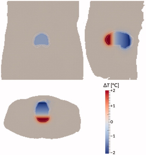
A second alternative, that follows more easily and logically from the current study, would be to assume perfect and immediate mixing of the bladder contents. As a comparison, we studied this model for patient #12. Computation times went down from 15.6 to 2.5 s per real time second, and with further optimization or improved hardware, it would probably be feasible to create a version that can simulate in real time, opening up new possibilities for in the treatment room. However, temperature differences between this ‘perfect mixing’ model and the dynamic model are not negligible: they ranged between roughly −2 and +2 °C, as is shown in Figure 10. The differences show a clear gradient in the vertical direction, showing the net heat transport against the direction of gravity, caused by convection. Improving this model by adding a simple heat transport term in the vertical direction, is subject of ongoing research.

Figure 10. Temperature difference between the dynamic model and the ‘perfect mixing’ model (‘perfect mixing’ minus dynamic) after 90 min treatment time for patient #12. Bladder wall shown in white. Shown are a coronal view (top right), sagittal view (top left), and axial view (bottom) through the centre of gravity of the bladder. Gravity points into the paper, to the left, and to the bottom, respectively.

The dynamic model presented in this article significantly improves temperature predictions of bladder (wall) temperatures, which provides opportunities for further clinically related research and improvement of quality assurance. As temperature is correlated to penetration depth of the chemotherapeutic instillation [50], future research will include a study of the relation between hyperthermic dose and clinical effect, taking into particular account the relation between temperatures measured in the bladder, the computed temperature in the bladder wall, and the therapeutic benefit.

In order to properly determine such a dose effect relation, and also for quality assurance in general, it is important to know the clinically relevant tumor temperature. In the case of bladder cancer there are generally no temperature sensors inserted into the tumor or bladder wall, and treatment target temperature is therefore not measured directly; consequently, it is evident that this should be modeled as accurately as possible. It is no less important to properly model the bladder lumen temperature, though, as that is the quantity that is actually measured, and which can therefore be used to assess the quality of the simulations, and correct them as needed.

A clear advantage of the dynamic model is its predicted robustness. The temperature sensor positions need not be known extremely precisely, as the homogenizing effect of convection inside the bladder results in a fairly homogeneous temperature distribution. Moreover, the convection in the bladder contents leads to a very good correlation between volumetric temperature measures like the T₅₀ of the measurements inside the bladder lumen and the T₅₀ of the bladder wall. For the same reason, a limited number of measurement points in the bladder will generally be sufficient to give a good understanding of the bladder wall temperature.

Conclusions

The new convective bladder model drastically improves accuracy of temperature predictions in the urinary bladder compared to the previously used model, which used the same equations to simulate both urine and muscle. The mean error in the clinically highly relevant predicted T₅₀ is reduced from 3.8 °C to 0.6 °C, and improved SAR computations are likely to reduce that even further. The bladder wall thermal dose parameters were shown to be very strongly correlated to the bladder lumen’s parameters, allowing to determine the tumor temperature with good accuracy, even based on a limited number of sensors in the bladder.

Disclosure statement

No potential conflict of interest was reported by the authors.

Additional information

Funding

The KWF Dutch Cancer Society financially supported this work, Grant No. UVA 2012–5539.

References

- Liem EIML, Crezee H, de la Rosette JJMCH, et al. Chemohyperthermia in non-muscle-invasive bladder cancer: an overview of the literature and recommendations. Int J Hyperthermia. 2016;32:363–373.
- Sousa A, Piñeiro I, Rodríguez S, et al. Recirculant hyperthermic IntraVEsical chemotherapy (HIVEC) in intermediate–high-risk non-muscle-invasive bladder cancer. Int J Hyperthermia. 2016;32:374–380.
- van Valenberg H, Colombo R, Witjes JA. Intravesical radiofrequency induced hyperthermia for non-muscle-invasive bladder cancer. Int J Hyperthermia. 2016;32:351–362.
- van Valenberg FJP, van der Heijden AG, Lammers RJM, et al. Intravesical radiofrequency induced hyperthermia enhances mitomycin C accumulation in tumour tissue. Int J Hyperthermia. 2017;1:1–6.
- Wittlinger M, Rödel CM, Weiss C, et al. Quadrimodal treatment of high-risk T1 and T2 bladder cancer: transurethral tumor resection followed by concurrent radiochemotherapy and regional deep hyperthermia. Radiother Oncol J Eur Soc Ther Radiol Oncol. 2009;93:358–363.
- Datta NR, Eberle B, Puric E, et al. Is hyperthermia combined with radiotherapy adequate in elderly patients with muscle-invasive bladder cancers? Thermo-radiobiological implications from an audit of initial results. Int J Hyperthermia. 2016;32:390–397.
- Longo TA, Gopalakrishna A, Tsivian M, et al. A systematic review of regional hyperthermia therapy in bladder cancer. Int J Hyperthermia. 2016;32:381–389.
- Franckena M, Fatehi D, de Bruijne M, et al. Hyperthermia dose-effect relationship in 420 patients with cervical cancer treated with combined radiotherapy and hyperthermia. Eur J Cancer. 2009;45:1969–1978.
- Cox RS, Kapp DS. Correlation of thermal parameters with outcome in combined radiation therapy–hyperthermia trials. Int J Hyperthermia. 1992;8:719–732.
- Oleson JR, Samulski TV, Leopold KA, et al. Sensitivity of hyperthermia trial outcomes to temperature and time: Implications for thermal goals of treatment. Int J Radiat Oncol Biol Phys. 1993;25:289–297.
- Rau B, Wust P, Tilly W, et al. Preoperative radiochemotherapy in locally advanced or recurrent rectal cancer: Regional radiofrequency hyperthermia correlates with clinical parameters. Int J Radiat Oncol Biol Phys. 2000;48:381–391.
- Stoll AM, Greene LC. Relationship between pain and tissue damage due to thermal radiation. J Appl Physiol. 1959;14:373–382.
- Kok HP, Korshuize-van Straten L, Bakker A, et al. Online adaptive hyperthermia treatment planning during locoregional heating to suppress treatment-limiting hot spots. Int J Radiat Oncol Biol Phys. 2017;99:1039–1047.
- Babjuk M, Böhle A, Burger M, et al. EAU guidelines on Non-Muscle-invasive Urothelial Carcinoma of the Bladder: Update 2016. Eur Urol. 2017;71:447–461.
- Colombo R, Salonia A, Leib Z, et al. Long-term outcomes of a randomized controlled trial comparing thermochemotherapy with Mitomycin-C alone as adjuvant treatment for non-muscle-invasive bladder cancer (NMIBC). BJU Int. 2011;107:912–918.
- Arends TJH, Nativ O, Maffezzini M, et al. Results of a randomised controlled trial comparing intravesical chemohyperthermia with mitomycin C versus bacillus calmette-guerin for adjuvant treatment of patients with intermediate- and high-risk non–muscle-invasive bladder cancer. Eur Urol. 2016;69:1046–1052.
- Geijsen ED, de Reijke TM, Koning CC, et al. Combining mitomycin C and regional 70 MHz hyperthermia in patients with nonmuscle invasive bladder cancer: a pilot study. J Urol. 2015;194:1202–1208.
- Inman BA, Stauffer PR, Craciunescu OA, et al. A pilot clinical trial of intravesical mitomycin-C and external deep pelvic hyperthermia for non-muscle-invasive bladder cancer. Int J Hyperthermia. 2014;30:171–175.
- A phase II, open label, multicenter randomised controlled trial comparing hyperthermia plus mitomycin to mitomycin alone, in patients with intermediate risk non-muscle invasive bladder cancer (ISRCTN 23639415). Available from: http://www.isrctn.com/ISRCTN23639415. Accessed December 22, 2017
- Owusu RA, Abern MR, Inman BA. Hyperthermia as adjunct to intravesical chemotherapy for bladder cancer. Biomed Res Int. 2013;2013:2013:262313
- Mikhail AS, Negussie AH, Pritchard WF, et al. Lyso-thermosensitive liposomal doxorubicin for treatment of bladder cancer. Int J Hyperthermia. 2017;33:1–740.
- Oliveira MB, Nova MV, Bruschi ML. A review of recent developments on micro/nanostructured pharmaceutical systems for intravesical therapy of the bladder cancer. Pharm Dev Technol. 2018;23:1–12.
- Stauffer PR, van Rhoon GC. Overview of bladder heating technology: matching capabilities with clinical requirements. Int J Hyperthermia. 2016;32:407–416.
- van der Heijden A, Kiemeney L, Gofrit O, et al. Preliminary European results of local microwave hyperthermia and chemotherapy treatment in intermediate or high risk superficial transitional cell carcinoma of the bladder. Eur Urol. 2004;46:65–72.
- van Dijk JD, Schneider C, van Os R, et al. Results of deep body hyperthermia with large waveguide radiators. Adv Exp Med Biol. 1990;267:315–319.
- Turner PF. Regional hyperthermia with an annular phased array. IEEE Trans Biomed Eng. 1984;31:106–114.
- Kok HP, Ciampa S, de Kroon-Oldenhof R, et al. Toward online adaptive hyperthermia treatment planning: correlation between measured and simulated specific absorption rate changes caused by phase steering in patients. Int J Radiat Oncol Biol Phys. 2014;90:438–445.
- Kok HP, Korshuize-van Straten L, Bakker A, et al. Feasibility of on-line temperature-based hyperthermia treatment planning to improve tumour temperatures during locoregional hyperthermia. Int J Hyperthermia. 2017;1–10.
- Kok HP, Wust P, Stauffer PR, et al. Current state of the art of regional hyperthermia treatment planning: a review. Radiat Oncol. 2015;10: 196.
- Paulides MM, Stauffer PR, Neufeld E, et al. Simulation techniques in hyperthermia treatment planning. Int J Hyperthermia. 2013;29:346–357.
- Balidemaj E, Kok HP, Schooneveldt G, et al. Hyperthermia treatment planning for cervical cancer patients based on electric conductivity tissue properties acquired in vivo with EPT at 3T MRI. Int J Hyperthermia. 2016;32:558–568.
- Yuan Y, Cheng KS, Craciunescu OI, et al. Utility of treatment planning for thermochemotherapy treatment of nonmuscle invasive bladder carcinoma. Med Phys. 2012;39:1170–1181.
- Schooneveldt G, Kok HP, Geijsen ED, et al. Improved temperature monitoring and treatment planning for loco-regional hyperthermia treatments of non-muscle invasive bladder cancer (NMIBC). In: Jaffray DA, editor. World Congress on Medical Physics and Biomedical Engineering, June 7–12, 2015, Toronto, Canada: Springer, 2015, pp. 1691–1694.
- Schooneveldt G, Kok HP, Balidemaj E, et al. Improving hyperthermia treatment planning for the pelvis by accurate fluid modeling. Med Phys. 2016;43:5442
- Kok HP, Kotte ANTJ, Crezee J. Planning, optimisation and evaluation of hyperthermia treatments. Int J Hyperthermia. 2017;33:593–607.
- Schooneveldt G, Bakker A, Balidemaj E, et al. Thermal dosimetry for bladder hyperthermia treatment. An overview. Int J Hyperthermia. 2016;32:417–433.
- Balidemaj E, de Boer P, van Lier ALHMW, et al. In vivo electric conductivity of cervical cancer patients based on B1+ maps at 3 T MRI. Phys Med Biol. 2016;61:1596–1607.
- de Leeuw AA, Crezee J, Lagendijk JJ. Temperature and SAR measurements in deep-body hyperthermia with thermocouple thermometry. Int J Hyperthermia. 1993;9:685–697.
- Hakenberg OW, Linne C, Manseck A, et al. Bladder wall thickness in normal adults and men with mild lower urinary tract symptoms and benign prostatic enlargement. Neurourol Urodyn. 2000;19:585–593.
- Kanyilmaz S, Calis FA, Cinar Y, et al. Bladder wall thickness and ultrasound estimated bladder weight in healthy adults with portative ultrasound device. J Res Med Sci. 2013;18:103–106.
- van der Koijk JF, Crezee J, Lagendijk JJ. Thermal properties of capacitively coupled electrodes in interstitial hyperthermia. Phys Med Biol. 1998;43:139–153.
- Carnochan P, Dickinson RJ, Joiner MC. The practical use of thermocouples for temperature measurement in clinical hyperthermia. Int J Hyperthermia. 1986;2:1–19.
- Kumar P, Kumar D, Rai KN. Numerical simulation of dual-phase-lag bioheat transfer model during thermal therapy. Math Biosci. 2016 ;Nov 281:82–91.
- Taflove A. Computational electrodynamics: the finite-difference time-domain method. Artech House, Boston; 1995.
- Pennes HH. Analysis of tissue and arterial blood temperatures in the resting human forearm. J Appl Physiol. 1948;1:93–122.
- Weller HG, Tabor G, Jasak H, et al. A tensorial approach to computational continuum mechanics using object orientated techniques. Comput Phys. 1998;12:620–631.
- T. Holzmann, Mathematics, Numerics, Derivations and OpenFOAM® (2017). Available from: https://holzmann-cfd.de/publications/mathematics-numerics-derivations-and-openfoam/
- Schneider CJ, van Dijk JD, de Leeuw AA, et al. Quality assurance in various radiative hyperthermia systems applying a phantom with LED matrix. Int J Hyperthermia. 1994;10:733–747.
- Kell GS. Density, thermal expansivity, and compressibility of liquid water from 0° to 150°. Correlations and tables for atmospheric pressure and saturation reviewed and expressed on 1968 temperature scale. J Chem Eng Data. 1975;20:97–105.
- van der Heijden AG, Dewhirst MW. Effects of hyperthermia in neutralising mechanisms of drug resistance in non-muscle-invasive bladder cancer. Int J Hyperthermia. 2016;32:434–445.
- Balidemaj E, van Lier ALHMW, Crezee H, et al. Feasibility of electric property tomography of pelvic tumors at 3T. Magn Reson Med. 2015;73:1505–1513.
- Gabriel C, Gabriel S, Corthout E. The dielectric properties of biological tissues: I. Literature survey. Phys Med Biol. 1996;41:2231–2249.
- Gabriel S, Lau RW, Gabriel C. The dielectric properties of biological tissues: II. Measurements in the frequency range 10 Hz to 20 GHz. Phys Med Biol. 1996;41:2251–2269.
- Gabriel C, Gabriel S. Compilation of the dielectrical properties of body tissues at rf and microwave frequencies. Texas: Armstrong Laboratory, Brooks Air Force Base; 1996.
- Rossmann C, Haemmerich D. Review of temperature dependence of thermal properties, dielectric properties, and perfusion of biological tissues at hyperthermic and ablation temperatures. Crit Rev Biomed Eng. 2014;42:467–492.
- Klein L, Swift C. An improved model for the dielectric constant of sea water at microwave frequencies. IEEE Trans Antennas Propagat. 1977;25:104–111.
- Sharqawy MH, Lienhard JH, Zubair SM. Thermophysical properties of seawater: a review of existing correlations and data. Desalin Water Treat. 2010;16:354–380.