Real-time monitoring radiofrequency ablation using tree-based ensemble learning models

Abstract

Background: Radiofrequency ablation is a minimally-invasive treatment method that aims to destroy undesired tissue by exposing it to alternating current in the 100 kHz–800 kHz frequency range and heating it until it is destroyed via coagulative necrosis. Ablation treatment is gaining momentum especially in cancer research, where the undesired tissue is a malignant tumor. While ablating the tumor with an electrode or catheter is an easy task, real-time monitoring the ablation process is a must in order to maintain the reliability of the treatment. Common methods for this monitoring task have proven to be accurate, however, they are all time-consuming or require expensive equipment, which makes the clinical ablation process more cumbersome and expensive due to the time-dependent nature of the clinical procedure.

Methods: A machine learning (ML) approach is presented that aims to reduce the monitoring time while keeping the accuracy of the conventional methods. Two different hardware setups are used to perform the ablation and collect impedance data at the same time and different ML algorithms are tested to predict the ablation depth in 3 dimensions, based on the collected data.

Results: Both the random forest and adaptive boosting (adaboost) models had over 98% R² on the data collected with the embedded system-based hardware instrumentation setup, outperforming Neural Network-based models.

Conclusions: It is shown that an optimal pair of hardware setup and ML algorithm (Adaboost) is able to control the ablation by estimating the lesion depth within a test average of 0.3mm while keeping the estimation time within 10ms on a ×86–64 workstation.

Keywords:

• Radiofrequency
• ablation
• tumor
• cancer
• control
• monitoring
• machine
• learning
• ensemble
• lesion
• depth

1. Introduction

Ablation is a type of therapy in which the undesired part of a tissue is removed by different methods. Realizing this task with minimal invasion is the main objective in many medical research fields. In cancer treatment, the undesired tissues are tumors, benign or malignant, and they are surrounded by healthy tissue, which is theoretically not supposed to be affected by the ablation. Hence, the second (and just as important) objective in cancer treatment is controlling/monitoring the ablation so that the treatment gets as close as possible to the ideal case where all cancerous cells are destroyed and all healthy cells remain intact. Even though open surgery is still the golden standard for removing cancerous tissues from various organs, minimally invasive ablation techniques with a fast and efficient monitoring method has gained more popularity especially because of their patient-friendly approach.

Radiofrequency ablation (RFA) is a minimally-invasive thermal ablation method and widely used in tumor ablation. The cancerous tissue is reached either by electrodes or a catheter and an alternating current (AC) passing through them causes excitation and motion of intracellular ions and hence, thermal heating within the tissue. Above a certain temperature for a given time of exposure, this heating results in the coagulative necrosis of the tumor cells. RFA is applied to the treatment of a variety of solid tumors [1,2]. In particular, RFA has gained the most popularity in risky surgical operations such as with Hepatocellular Carcinoma (HCC) treatment and lung nodule removal [3–5]. More recently, RFA has started to be offered as a solid approach to breast cancer treatment that will be the main focus of this study by simulating breast tissue and collecting data from it [6]. Even though open surgery is still the golden standard for breast tumors, RFA is becoming a solid alternative, especially when surgery is not an option. RFA is also being used in combination with surgery in some studies, in order to achieve total destruction of the tumor and avoid recurrence [7].

RFA treatment can start to create some physiological problems if applied without a proper monitoring mechanism due to the uncontrollable nature of thermal ablation [8]. The main aspect to be monitored is the extent of the ablation zone as the AC is applied. It should be made sure that all cancerous volume is ablated and as much healthy tissue as possible is left intact at the end of the ablation process. The ablation volume is mostly related to the temperature distribution in the target tissue. Above 100 °C, the water inside the tissue begins to vaporize, decreasing the thermal and electrical conductivity of the tissue, potentially stopping the ablation process [9]. Furthermore, even though enough RF current is delivered, some parts of the target tissue may sometimes stay under the necessary temperature threshold for ablation to start, due to the ‘heat-sink’ effect of a nearby vascular structure, which carries away some of the given thermal energy with the local blood flow [10]. Therefore, it is essential that RFA should be accompanied by a real-time monitoring scheme in order to make sure that there is no unablated volume left in the tumor that can cause recurrence or too much ablated healthy tissue that would lead to deformation or even total destruction of the tissue.

As of 2018, there is a significant amount of research done to develop a low-cost, efficient, and accurate real-time monitoring scheme for RFA. Since visual and noninvasive monitoring is virtually impossible due to the opacity of the cancerous tissue, many techniques utilize the changes in tissue properties; more specifically electrical, optical and acoustic behavior under the ablation treatment. For acoustic imaging, the acoustic waves traveling from the target tissue are used. The acoustic waves are emitted and received by an acoustic device that is also used as a sensor [11]. Gas bubbles induced during RFA due to evaporation of heated tissue content can interfere with this kind of imaging. To solve this problem, Nagakami imaging is applied and an enhanced ablation zone visualization is obtained [12]. More recently, an adaptive ultrasound imaging scheme is applied to obtain better depth estimations with an algorithm that adjusts its parameters with changing medium properties, like temperatures higher than 50 °C [13]. Yet another technique is optoacoustic imaging that uses an optical device that emits laser pulses to excite the target tissue and uses sensors to collect the acoustic emission data from these pulses [14,15]. As for using electrical behavior, electrical complex impedance of the targeted tissue is measured. Electrical impedance tomography (EIT), one of the methods that utilize the measured electrical impedance for monitoring RFA, uses electrodes surrounding the targeted tissue to measure impedance paths [16]. The data collected in EIT are then reconstructed into tissue electrical conductivity and temperature to provide lesion depth images [17–19]. The principle that allows for electrical impedance to be utilized is the temperature dependence of the electrical conductivity of biological tissue [20].

For all methods explained above that use tissue properties, sufficient data can be collected very fast, with speeds higher than 10 Hz because they only depend on the speed of the setup and the equipment. However, the reconstruction of a depth map requires more time to be accurate. Absolute EIT imaging essentially requires solving an optimization problem overlaid onto an ill-posed three-dimensional finite element modeling (FEM) problem, which is fairly complex. Thus, computing a single EIT-based lesion depth map requires time on the order of tens of seconds and minutes (100+ seconds at 90%+ accuracy on an ×86 processor-based workstation) [21]. Space-wise, computing an EIT lesion depth map can potentially occupy 1+ gigabyte of memory due to the reconstruction mesh size [12,18,19]. An optoacoustic imaging step requires 400+ seconds to reach 95% accuracy with a similar tomographic reconstruction algorithm [18]. One novelty of this study is collecting data with different setups that are inspired by the EIT model and then instead of reconstructing a depth map, analyzing the data with a Machine Learning (ML) approach that gives an estimation very quickly once the model is trained with sufficient data. Different ensemble models will be tested and it is shown that with the combination of the proper data collection setup and the ML algorithm, the accuracy of current monitoring methods can be beaten while drastically cutting the time to obtain depth predictions.

Especially after the computational capacity of computers are increasingly enhanced, ML finds itself applications in numerous fields, including medicine and biomedical engineering [22,23]. Bayesian regression with Gaussian Processes proved to be useful for the analysis of time series data collected from sensors on patients [24]. For tasks with structured data and a moderate number of variables (i.e., with a low-dimensional dataset), classical methods like Decision Trees and Support Vector Machines (SVMs) have been used and performed quite well. A SVM model has been used to classify patients with diabetes and pre-diabetes based on their personal health information [25]. Another study shows the use of SVMs for predicting medication adherence in heart-failure patients [26]. A Decision Tree model has been used to predict early rejection in kidney transplant [27]. More recently, Artificial Neural Networks (ANNs) and models based on their framework are preferred for applications that include audial or/and visual data because of the high dimensionality and complexity of images, videos and recordings. With a high number of parameters and being able to utilize non-linearities, ANNs can capture the complexity in high-dimensional data successfully. In cancer research, ANNs with many layers, also referred as ‘Deep networks’ are used to classify cancers into diagnostic subgroups based on the gene expression profiling data of the patients [28]. Networks with a specialized architecture for image processing, Convolutional Neural Networks (CNN) are gaining momentum for classifying patients with or without breast cancer based on their mammogram images [29]. Another breakthrough of CNNs in cancer diagnosis was showing a detection performance of skin cancer on par with expert dermatologists by training on lesion photographs of more than 1 million patients [30]. All in all, applications of ML onto medical research mostly consist of analyzing data collected either before or after the treatment. Another novelty of this study is using ML for data that is collected during the ablation treatment and developing algorithms that once trained, can give fast and accurate predictions during the treatment as well, not before it starts or after it is completed.

The work most related to this study would be a pseudo-EIT method published in Wang et al’s study [31] that utilizes electrical impedance, but rather than reconstruct the entire model as with EIT, an ANN was used as a depth estimation system that approximates the lesion depth map solution. The ensemble models that will be introduced in this study are predicted to outperform the ANN model for reasons that are thoroughly discussed in Section 2.2. Another extension of this study is using regression which directly predicts the ablation depth as opposed to the classification model in Wang et al’s study [31]. Section 2.2 explains why this is a safer approach than classification for a real-life scenario of monitoring ablation therapy. For comparison reasons, the ANN in Wang et al’s study [31] is retrained as a regression model alongside with different network architectures. The results from all the models will be presented and compared in Section 3. Yet another contribution of this study is the comparison of the original off-the-shelf system to a low-cost embedded system designed specifically for the measurement, computation and actuation of this system.

 Google Scholar

2. Materials and methods

2.1. Hardware configurations and data collection methods

The ablation is performed and complex impedance data were collected using the tissue model and the RFA hardware setup as in Wang et al’s study [31]. The model consisted of pork loin and pork belly, simulating breast tissue. The complex impedance data were collected by the same RFA device that performs the ablation, removing the need for any additional equipment for measurements that will add complexity to the patient setup. The true levels of ablation depth for training data were measured by temperature probes that were inserted into the tissue model on all six ablation faces. The temperature data for each direction after ablation was recorded using temperature probes that used platinum 100 Ω resistance temperature detectors. These detectors were placed at 0 mm, 5 mm, 10 mm and 15 mm depths from the side of the ablation device. The temperature values for the depths in between were linearly interpolated. After the temperature was recorded for all depth values from 0.0 mm to 15.0 mm with a step size of 0.1 mm, tissue volumes at 43 °C for $\ge$10 min, 50 °C for $\ge$5 min and 57 °C for $\ge$2 s were considered ablated and the lesion depth was calculated. These thresholds for temperature and exposure duration were determined with a literature review on cell death in RFA studies [15,32]. The model and the RFA device are shown in Figure 1.

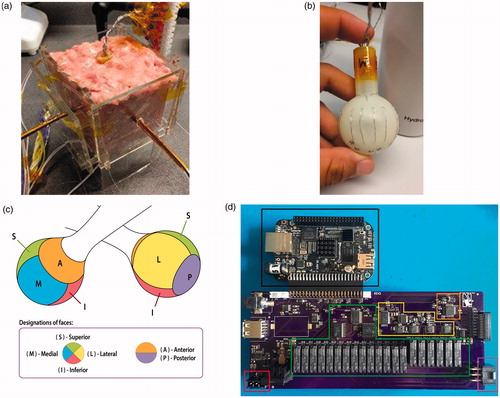
Figure 1. (a) The RFA tissue setup is shown with temperature probes inserted into each face of the device. (b) The RFA device is shown, with electrodes grouped by face. (c) The RFA device face partitioning on the surface of the device. (d) The new instrumentation system is shown, with the red box showing the RF generator connection socket, the green box showing the relay-based electrode switching subsystem, the yellow box showing the impedance analyzer subsystem, the orange box showing an auxiliary temperature measurement subsystem, and the purple box showing the RFA device connection socket.

The data collection was performed with two different sets of equipment. For the first dataset, off-the-shelf equipment was used. The system consisted of a matrix switch module as the electrode switching subsystem and an external LCR (Inductance (L), Capacitance (C), and Impedance (R)) meter as the impedance measurement subsystem. The LCR meter (Rohde & Schwartz HM8118) costs $2500 by itself. These measurement peripherals were controlled by a ×86–64 microprocessor-based workstation (Supermicro, San Jose, CA) with 16 GB of memory. This first dataset that was collected with this equipment and on which the results of Wang et al’s study [31] are based, is named as ‘first instrumentation data’.

For the second dataset, instead of the off-the-shelf equipment, a new low-cost embedded system was designed. The system includes an accessory board for a Beaglebone Black (Texas Instruments, Dallas, TX) and costs <$250 for the parts, including the integrated circuits, accessory board printed circuit board and microcontroller board. This accessory board combines a relay-based electrode switching subsystem and impedance analyzer subsystem. The complex electrical impedance measurement subsystem based on the AD5933 (Analog Devices, Norwood, MA) impedance analyzer integrated circuit instead of an external LCR meter. This apparatus design has a few advantages over the first design that is composed of off-the-shelf elements. First of all, the noise profile of the data is no longer dependent on signal chains through multiple external pieces of hardware. The data signals are collected in a consistent manner, not affected by any noise introduced by the wiring or interference of equipment not designed specifically for this purpose. This was clear with especially the LCR meter, which produced noisy results likely due to signal chains running through a matrix switch module in a chassis that also contained other modules. A visualization of the noise profile will be shown in Section 4 alongside how it is related to the results in this study. The embedded impedance measurement subsystem on the accessory board was designed to measure the impedance magnitude and phase within 2% error range for a frequency range from 10 kHz to 100 kHz, following the low-impedance-ranged CN-0217 reference design from Analog Devices. All complex impedance data presented in this study were measured at 100 kHz. The dataset collected with this new embedded system is the main contribution of this study in terms of ablation hardware, and is named as ‘second instrumentation data’. This second dataset will be compared with the first instrumentation dataset in terms of how much noise it contains. The accessory board design is shown in Figure 1.

As shown in Table 1, the first instrumentation collected 12,480 data points and the second instrumentation collected 10,344 data points from identical tissue models. Each sample ablation is comprised of 20–50 ablate/measure cycles. Each data measurement generates 6 samples per cycle (a pair of thermal and electrical impedance measurements per side).

Table 1. Number of data points and their distribution to different sets for regression data from both instrumentations.

	Number of data points
Dataset	Total	Training (at each fold)	Validation (at each fold)	Test
First Instrumentation	12480	7862	874	3744
Second Instrumentation	10344	6517	724	3103

The features were the same for both datasets. The four numerical features were the initial magnitude, the initial phase, the final magnitude and the final phase of the complex tissue impedance. Lastly, the activated face of the RFA device was added as a categorical feature. Since the integers that represent each category have a natural ordered relationship between each other unlike the categories in this dataset, this feature was one-hot-encoded into six binary features, adding up to ten dimensions in total. The target value to predict was the lesion depth in millimeters.

After both datasets were obtained, the prediction of the lesion depth was posed as a regression task. Although a comparison is beyond the scope of this study, we believe that approaching the ablation monitoring problem as a regression task is more of a direct approach to the problem, as this allows for the creation of a model that can directly produce a depth estimation without a linear or binary search. Additionally, as the classification task requires a linear or binary search to find the estimated depth, a single invalid output during the search can potentially produce a large error. The regression task allows for the direct fit and validation of the model to the training datasets.

2.2. The machine learning models

The ML models for lesion depth estimation are the ANN from Wang et al’s study [31] and two ensemble models that are introduced in this study: a Random Forest [33] and Adaptive Boosting [34]. There are few reasons for using tree-based ensemble learning models to make depth predictions from the complex impedance data. First of all, tree-based models have much fewer hyperparameters than ANNs, making them easier to tune and interpret after training. Secondly, they need less preprocessing to learn the data and they are able to process numerical and categorical features together successfully, which is not the case for many ML models [35]. Another reason that is more specific to this study is the format of the target values. Since there is a finite amount of leaf nodes, using a tree for a regression task returns predictions only at certain discrete values. The target values in this study are already such discrete depth values between 0 and 15 mm, with a step size of 0.1 mm, allowing a tree-based model to make accurate predictions. Moreover, using a number of trees as an ensemble takes away the instability problem of a single Decision Tree [36].

2.2.1. Artificial neural network

The ANN from Wang et al’s study [31] is used as a regressor instead of a classifier to enable a direct comparison between the tree-based ensemble models in this study. Different architectures were tried as the number of layers and nodes at each layer are tuned with the validation data. After a uniform grid search between 2 and 10 layers and 20–500 nodes per layer, it was verified that the architecture in Wang et al’s study [31] is the architecture that generalizes best to test data and should be kept as the first ML model.

2.2.2. Random Forest

A Random Forest has a Decision Tree as its base estimator, which is trained with the Classification and Regression Trees (CART) algorithm [33]. The algorithm is based on dividing the dataset into two subsets by setting the optimum threshold t_k along a randomly picked feature k. This is done by minimizing the following cost function: (1) $$J(k,t_k)=\frac{m_{\mathit{left}}}{m}MS{E}_{\mathit{left}}+\frac{m_{\mathit{right}}}{m}MS{E}_{\mathit{right}}$$(1) where m_left, MSE_left, m_right and MSE_right are the number and the mean squared error (MSE) of all the instances on the left and the right of the threshold point along the feature dimension k, respectively.

In the Random Forest, all decision trees work in parallel, trained only with a subset of the training data. This introduces predictor diversity and randomness so that the final model, which is called an ensemble, will not be affected by the data size or any change in the dataset. The predictions for the new instances are obtained by averaging all decisions of the trees in the forest. The training for a Random Forest is summarized in Algorithm 1.

Algorithm 1: Random Forest Algorithm

REQUIRE The feature matrix, the target values, the number of trees in the forest, maximum number of leaf nodes (chosen regularization criterion for this study)

n = 1;

REPEAT

     Pick a random subset of features;

     Among the chosen features, pick a feature k and a threshold t_k and start from the first node

     REPEAT

           Minimize $J\left(k, t_k\right)$ in Eq. 1(1) $$J(k,t_k)=\frac{m_{\mathit{left}}}{m}MS{E}_{\mathit{left}}+\frac{m_{\mathit{right}}}{m}MS{E}_{\mathit{right}}$$(1)

           Separate the data into two child nodes

           Pass onto the child nodes

     UNTIL Pure leaf nodes or regularization criterion met

     n = n + 1

UNTIL n = number of trees

2.2.3. Adaptive Boosting

Adaptive Boosting also has a Decision Tree as its base model, however, each tree is trained one by one and the algorithm makes each tree pay more attention to the data points the previous one missed. This is done by assigning a weight value to each instance in the dataset and changing these weights for each tree in the training sequence.

Initially, all instances start with the weights: (2) $$w^{\left(i\right)}=1/m$$(2) where m is the size of the dataset and $w^{(i)}$ is the weight of the i^th instance. These weights are updated as a tree makes its predictions and the next tree is trained with the data and the updated weights. Each predictor in the model in this study is still a tree, so CART algorithm is used for each base predictor. The slight derivation to include the instance weights to the algorithm is made on the MSE calculation at a node, which is: (3) $$\mathit{MS}{E}_{\mathit{node}}=\sum _{i\in \mathit{node}}{w}^{\left(i\right)}{({\widehat{y}}_{\mathit{node}}-y^{\left(i\right)})}^2$$(3)

After training the j^th tree, its error rate is calculated as follows: (4) $$r_j=\frac{\sum _{{\widehat{y}}_j^{\left(i\right)}\ne y^{\left(i\right)}}^{m}i=1w^{\left(i\right)}}{\sum _{i=1}^m{w}^{\left(i\right)}}$$(4) where ${\widehat{y}}_j^{(i)}$ is the prediction of the j^th tree for the i^th data point.

Using the error rate, the predictor weight of the j^th tree is calculated as follows: (5) $${\alpha }_j=\eta \hspace{0.17em}\text{log}\hspace{0.17em}\left(\frac{1-r_j}{r_j}\right)$$(5) where η is the learning rate, an ensemble hyperparameter that should be manually tuned. Based on the weight of the j^th predictor, the data point weights are updated for ${(j+1)}^{\mathit{th}}$ the predictor to use as follows: (6) $$w^{\left(i\right)}\Rightarrow \{\begin{array}{cc}{w}^{\left(i\right)}\hfill & \text{if} {\widehat{y}}_j^{\left(i\right)}=y^{\left(i\right)}\hfill \\ w^{\left(i\right)}e\mathit{xp}\left({\alpha }_j\right)\hfill & \text{if} {\widehat{y}}_j^{\left(i\right)}\ne y^{\left(i\right)}\hfill \end{array}$$(6)

The weight updating and predictor training processes are repeated until all the predictors are trained. An important point for Adaptive Boosting is that the condition ${\widehat{y}}_j^{(i)}\ne y^{(i)}$ can be too strict for a regression task that predicts continuous target values with very small granularity. Since the target values are more discrete and within a small range for the regression task of this study, this is not regarded as a problem.

To make predictions for new instances, a weighted average of all the trees is taken, which can be formulated as: (7) $$\widehat{y}\left(\mathbf{x}\right)=\arg \underset{k}{\max }\sum _{{j=1}_{{\widehat{y}}_j}\left(\mathbf{x}\right)=k}^N{\alpha }_j$$(7) where $\widehat{y}(\mathbf{x})$ is the ensemble prediction for the new data point x, k is a target value and ${\widehat{y}}_j(\mathbf{x})$ is the prediction of the j^th predictor. The summary of the Adaptive Boosting algorithm is shown in Algorithm 2.

Algorithm 2: Adaptive Boosting Algorithm

REQUIRE: The feature matrix, total number of data points (m), the target values, total number of trees, maximum number of leaf nodes (chosen regularization criterion for this study), learning rate (fixed)

n = 1;

$$\mathit{ }{w}^{\left(i\right)}= \frac{1}{m}$$

REPEAT

     Pick a feature k and a threshold t_k and start from the first node

     REPEAT

           Minimize $J\left(k, t_k\right)$ in Eq. 1(1) $$J(k,t_k)=\frac{m_{\mathit{left}}}{m}MS{E}_{\mathit{left}}+\frac{m_{\mathit{right}}}{m}MS{E}_{\mathit{right}}$$(1)

           Separate the data into two child nodes

           Pass onto the child nodes

     UNTIL Pure leaf nodes or regularization criterion met

     Calculate $r_j$ using Eq. 4(4) $$r_j=\frac{\sum _{{\widehat{y}}_j^{\left(i\right)}\ne y^{\left(i\right)}}^{m}i=1w^{\left(i\right)}}{\sum _{i=1}^m{w}^{\left(i\right)}}$$(4)

     Calculate ${\alpha }_j$ using Eq. 5(5) $${\alpha }_j=\eta \hspace{0.17em}\text{log}\hspace{0.17em}\left(\frac{1-r_j}{r_j}\right)$$(5)

     Update $w^{\left(i\right)}$ using Eq. 6(6) $$w^{\left(i\right)}\Rightarrow \{\begin{array}{cc}{w}^{\left(i\right)}\hfill & \text{if} {\widehat{y}}_j^{\left(i\right)}=y^{\left(i\right)}\hfill \\ w^{\left(i\right)}e\mathit{xp}\left({\alpha }_j\right)\hfill & \text{if} {\widehat{y}}_j^{\left(i\right)}\ne y^{\left(i\right)}\hfill \end{array}$$(6)

     n = n + 1

UNTIL n = number of trees

The main shortcoming of tree-based models is that they are very susceptible to overfitting, where the prediction performance for previously unseen data gets much worse than the training data. This is avoided by regularization, which limits the complexity of the models so they do not overfit to the training data and are able to generalize well to new data. Regularization is done by limiting a hyperparameter of the model. For the models in this study, the number of maximum leaf nodes in each tree is picked as the regularization hyperparameter. Constraining this value for a tree makes it stop branching out as its number of leaf nodes reaches the limit, even if not all the leaf nodes are pure. The number of trees in the ensemble is another hyperparameter to be tuned and the complexity of the model depends on it as well.

Both tree-based models were created on the Scikit-learn Python library (INRIA, Rocquencourt, France). They were run on a ×86–64 microprocessor-based workstation (Supermicro, San Jose, CA) with 16 GB of memory. Both tree-based models were tested on both the first and second instrumentation data. Furthermore, their results are compared with those of the ANN in Wang et al’s study [31] that is retrained as a regression model.

3. Results

For both datasets and ML models, 70% of the data was used to train the model and tune the hyperparameters with a 10-fold cross-validation (CV). The other 30% was held out to test how well the trained models generalize to new data. The size of the training, validation and test sets for each dataset was shown in Table 1. Since the prediction task in this study is regression, root mean squared error (RMSE) and R² were used as evaluation metrics to compare the models, along with the residual plots of the ensemble models to visualize their prediction performance.

The hyperparameters to tune in both the Random Forest and the Adaptive Boosting model were the number of trees and the maximum number of leaf nodes in each tree. While the model parameters were tuned by the training data, these hyperparameters were optimized by a grid search. Since it is computationally very expensive to do a grid search for three hyperparameters at the same time, the learning rate of Adaptive Boosting was fixed to 0.1, a reasonable value found after trial and error, and the other two hyperparameters were put to the grid search. This also helped with a comparison between two ensemble models. Figure 2 has the grid search for the hyperparameters. For both models, the number of trees was fixed first to find the optimum number of leaf nodes and then this value is kept to tune the number of trees, which did not affect the prediction performance as much as the former. Figure 2 also enables a direct comparison between the datasets under the same hyperparameter values.

Figure 2. The grid search for the hyperparameters of both ensemble models with a comparison between the datasets. The criterion for the best hyperparameter value is the test R². a) Tuning the maximum number of leaf nodes for Random Forest. (Number of trees fixed at 80 for both models). b) Tuning the number of trees for Random Forest. (Max. number of leaf nodes fixed at 250 and 900 for the first and second instrumentation, respectively). c) Tuning the maximum number of leaf nodes for Adaptive Boosting. (Number of trees fixed at 30 for both models). d) Tuning the number of trees for Adaptive Boosting. (Max. number of leaf nodes fixed at 250 and 700 for the first and second instrumentation, respectively).

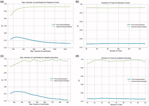
Table 2 has the results of all the models trained with the first instrumentation data. The Random Forest was trained with 80 trees and a maximum of 250 leaf nodes each. The Adaptive Boosting model had 30 trees and a maximum of 250 leaf nodes each.

Table 2. Output performances of all the ML models when cross-validated and tested on the first instrumentation data.

	Prediction metrics for regression
ML Model	Test RMSE (mm)	Test R^2	CV-average RMSE (mm)	CV-average R^2
ANN^a	2.45	68.1%	2.45	67.6%
Random Forest	2.16	77.2%	2.20	76.3%
Adaptive Boosting	2.08	79.3%	2.12	75.2%

Note: ^aThe same model and hyperparameters from [31].

Table 3 has the results of all the models trained with the second instrumentation data. The Random Forest was trained with 50 trees and a maximum of 900 leaf nodes each. The Adaptive Boosting model had 30 trees and a maximum of 700 leaf nodes each. For both datasets, the Random Forest finished training in 0.37 s and predicted the depths for test data in 0.01 s. With Adaptive Boosting, training took 3.3 s and prediction took 0.01 s again.

Table 3. Output performances of all the ML models when cross-validated and tested on the second instrumentation data.

	Prediction metrics for regression
ML Model	Test RMSE (mm)	Test R^2	CV-average RMSE (mm)	CV-average R^2
ANN^a	2.19	57.0%	2.23	56.0%
Random Forest	0.54	98.0%	0.62	96.2%
Adaptive Boosting	0.30	99.1%	0.51	97.5%

Note: ^aThe same model and hyperparameters from [31].

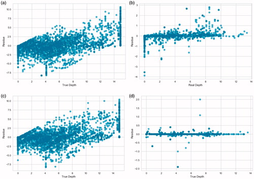
Lastly, the residual plots of both ensemble models introduced in this study are shown in Figure 3. The residual plots were obtained from the results of both instrumentations setups.

Figure 3. Residual plots of the predictions of the ensemble models on the test data from both instrumentations. The 0.0 mm depth is the tissue directly abutting the surface of the RFA device face. a) Random Forest on the first instrumentation data. b) Random Forest on the second instrumentation data. c) Adaptive Boosting on the first instrumentation data. d) Adaptive Boosting on the second instrumentation data.

4. Discussion

The first comparison is made between the two instrumentation setups. All metrics show that the second instrumentation data can be predicted more accurately, indicating the lack of noise, which is clearly not the case for the first instrumentation. The noise from the off-the-shelf equipment of the first instrumentation manifests itself through the inaccuracy of all the ML models. Both ensemble models have a test RMSE higher than 2 mm, which drops to around 0.5 mm with the new instrumentation. The reason for this sudden increase of the model performance is that the data size from both instrumentations are moderate for training ML models as complex as the ones in this study, so the effect of the noise could not be compensated by a large dataset.

Another indication of the noise in the first instrumentation from a ML perspective is the regularization hyperparameters of the ensemble models. It is especially notable that the number of maximum leaf nodes in both models has to be kept smaller while training them with the first instrumentation data. A tree-based ensemble model with a lower limit on its maximum leaf nodes is more strictly regulated and limited in complexity to avoid overfitting, which noisy training data are usually prone to causing. Therefore, both models are regulated to avoid overfitting and to keep the test results from dropping significantly. The overfitting for the first instrumentation data can be seen in Figure 2, as the R² for test data start to decrease as the number of maximum leaf nodes pass the optimum value, whereas the second instrumentation data maintains its peak R² as the number of leaf nodes increase. In other words, with the second instrumentation, both the Random Forest and the Adaptive Boosting models are allowed to have more leaf nodes and less regulation, which leads to better training and test performance because the noise is eliminated and the complexity the models are capturing belongs to the clean data itself, not the noise.

The noise difference between two datasets can also be seen from a biological perspective. As the lesion depth increases with more heat in the tissue model, the increasing temperature decreases the complex impedance. So, the impedance magnitude of the instances should follow a decreasing pattern when they are plotted against their corresponding lesion depth. These plots for both the impedance magnitude and phase are shown in Figure 4.

Figure 4. Magnitude and phase plots of datasets from both instrumentation setups. Face ablated lesion depth is the depth of the ablation lesion relative to a face of the RFA device. The 0.0 mm depth is the tissue directly abutting the surface of the RFA device face. a) Magnitude vs. depth for the first instrumentation. b) Magnitude vs. depth for the second instrumentation. c) Phase vs. depth for the first instrumentation. d) Phase vs. depth for the second instrumentation.

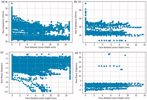
As the lesion depth increases, the magnitude follows two patterns around 40 and 20 Ω which is expected, as one pattern is for pork belly and the other is for pork loin. The magnitudes of different measurements that correspond to the same depth are expected to be within a tight margin. However, the impedance magnitudes for the first instrumentation are scattered and noisy, the patterns of two different materials merging at some depths, indicating the presence of noise introduced by the off-the-shelf LCR meter. The phase plot for the first dataset has the same issues, having the phase values more scattered than that of the second dataset, except for a few outliers that are caused by incorrect measurements by the accessory board.

The second comparison is made between the two tree-based ML models. Both tree-based ensemble models that are introduced in this study outperformed the ANN in Wang et al’s study [31]. The discrete nature of the target depth values certainly helped with the higher performance of the tree-based models. This shows that tree-based models can prove useful for various medical applications when there is a depth estimation involved as long as sufficient training data including all discrete depth levels is given. Furthermore, the tree-based ensemble models have less parameters to tune and faster to train, so for this study, it is safe to say they are more advantageous than an ANN. As for the comparison between the Random Forest and the Adaptive Boosting models, there are a few tradeoffs. First, the overall prediction performance of the Adaptive Boosting model is better than the Random Forest, with lower MSE, higher R² and a tighter residual plot for both datasets. This better prediction performance comes with a computational cost. Again for both datasets, the Adaptive Boosting model takes more than ten times as much time as the Random Forest model to train. This is expected because all the trees in the Adaptive Boosting model are trained sequentially on the entire dataset, whereas data is processed in parallel in the Random Forest. Therefore, the difference in training time between the models increases with more data. Another possible factor that would increase the computational cost of the Adaptive Boosting model is the additional learning rate hyperparameter to tune, which was fixed to 0.1 in this study.

Lastly, there are some visible patterns on the 4 residual plots in Figure 3. Both residual plots of the first instrumentation data have vertical patterns on 0 and 15 mm depth which correspond to a non-zero ablation depth prediction whereas the real depth is zero and a prediction of 15 mm depth when the thermal lesion is not there yet, respectively. There are also diagonal patterns stemming from 0 mm in depth. These correspond to the model predicting zero depth when there is some ablated volume. These inaccuracies would cause serious medical issues in real-life tumor ablation such as a recurrent cancer from unablated tumor volume or ablated healthy tissue volume that can lead to the collapse of an organ or body deformation. With the second instrumentation, the noise that causes these patterns of inaccuracy is gone. The diagonal pattern and the vertical pattern at 15 mm depth disappear but the one at 0 mm depth persists for the Random Forest model. This is likely due to a bigger proportion of the instances having 0 mm as the target depth and the Random Forest model missing some of them even when the noise is gone. The Adaptive Boosting model predicts the instances with 0 mm depth much better, returning a tighter residual plot with only random outliers. This is the last and probably the most important advantage the Adaptive Boosting model has for this study.

5. Conclusion

The results of this study show that a real-time monitoring for tumor ablation can be accurately done with an ML approach that is much faster than other monitoring techniques. Both the Random Forest and the Adaptive Boosting model proved useful and accurate, the latter having the most accurate depth predictions on average. An essential part of this process is a noise-free and reliable data collection setup, as demonstrated with the difference in prediction performance between the datasets of two different instrumentation hardware setups. Future studies will explore utilizing complex impedance data collected at multiple frequencies which will allow collecting a much bigger dataset and more useful new features. Also, it will enable the development of a more complex ML model that can predict the lesion depth more precisely.

Disclosure statement

In accordance with Taylor & Francis policy and ethical obligation as researchers, we are reporting that Y.C. Wang and T.C. Chan have financial interests in Innoblative Designs, Inc. that may be affected by the research reported in the enclosed paper. These interests have been disclosed fully to Taylor & Francis, and an approved plan for managing any potential conflicts arising from this arrangement is in place.

Additional information

Funding

This work was supported by the National Science Foundation under [grant number 1738541].

References

- Shah DR, Green S, Elliot A, et al. Current oncologic applications of radiofrequency ablation therapies. WJGO. 2012;5:71.
- Brace CL. Radiofrequency and microwave ablation of the liver, lung, kidney, and bone: what are the differences? Curr Probl Diagn Radiol. 2009;38:135–143.
- Tateishi R, Shiina S, Teratani T, et al. Percutaneous radiofrequency ablation for hepatocellular carcinoma: an analysis of 1000 cases. Cancer. 2005;103:1201–1209.
- Shiina S, Teratani T, Obi S, et al. A randomized controlled trial of radiofrequency ablation with ethanol injection for small hepatocellular carcinoma. Gastroenterology. 2005;129:122–130.
- Dupuy DE, Zagoria RJ, Akerley W, et al. Percutaneous radiofrequency ablation of malignancies in the lung. Ajr Am J Roentgenol. 2000;174:57–59.
- Kunkle DA, Uzzo RG. Cryoablation or radiofrequency ablation of the small renal mass: a meta-analysis. Cancer. 2008;113:2671–2680.
- Abdalla EK, Vauthey JN, Ellis LM, et al. Recurrence and outcomes following hepatic resection, radiofrequency ablation, and combined resection/ablation for colorectal liver metastases. Ann Surg. 2004;239:818.
- Wi H, McEwan AL, Lam V, et al. Real-time conductivity imaging of temperature and tissue property changes during radiofrequency ablation: an ex vivo model using weighted frequency difference. Bioelectromagnetics. 2015;36:277–286.
- Chu KF, Dupuy DE. Thermal ablation of tumours: biological mechanisms and advances in therapy. Nat Rev Cancer. 2014;14(3):199–208.
- Lu DS, Raman SS, Vodopich DJ, et al. Effect of vessel size on creation of hepatic radiofrequency lesions in pigs: assessment of the “heat sink effect”. Ajr Am J Roentgenol. 2002;178:47–51.
- Sliwa JW, Ma Z, Goetz JP, et al. Apparatus and methods for acoustic monitoring of ablation procedures. United States patent application US 12/636,837. 2010 Jul 1.
- Zhou Z, Wu S, Wang CY, et al. Monitoring radiofrequency ablation using real-time ultrasound nakagami imaging combined with frequency and temporal compounding techniques. PLoS One. 2015;10:e0118030.
- Liu YD, Li Q, Zhou Z, et al. Adaptive ultrasound temperature imaging for monitoring radiofrequency ablation. PloS One. 2017;12:e0182457.
- Pang GA, Bay E, Deán-Ben XL, et al. Three-dimensional optoacoustic monitoring of lesion formation in real time during radiofrequency catheter ablation. J Cardiovasc Electrophysiol. 2015;26:339–345.
- Larina IV, Larin KV, Esenaliev RO. Real-time optoacoustic monitoring of temperature in tissues. J Phys D: Appl Phys. 2005;38:2633.
- Holder DS, editor. Electrical impedance tomography: methods, history and applications. Boca Raton (FL): CRC Press; 2004.
- Wi H, McEwan AL, Lam V, et al. Real-time conductivity imaging of temperature and tissue property changes during radiofrequency ablation: an ex vivo model using weighted frequency difference. Bioelectromagnetics. 2015;36(4):277–286.
- Cherepenin VA, Karpov AY, Korjenevsky AV, et al. Three-dimensional EIT imaging of breast tissues: system design and clinical testing. IEEE Trans Med Imag. 2002;21(6):662–667.
- Javaherian A, Soleimani M, Moeller K. A fast time-difference inverse solver for 3D EIT with application to lung imaging. Med Biol Eng Comput. 2016;54(8):1243–1255.
- Chang I. Finite element analysis of hepatic radiofrequency ablation probes using temperature-dependent electrical conductivity. Biomed Eng Online. 2003;2:12.
- Martin S, Choi CT. A post-processing method for three-dimensional electrical impedance tomography. Sci Rep. 2017;7(1):7212.
- Magoulas GD, Prentza A. Machine learning in medical applications. Advanced course on artificial intelligence; Berlin, Heidelberg: Springer; 1999. p. 300–307.
- Foster KR, Koprowski R, Skufca JD. Machine learning, medical diagnosis, and biomedical engineering research-commentary. Biomed Eng Online. 2014;13:94.
- Durichen R, Pimentel MA, Clifton L, et al. Multi-task Gaussian process models for biomedical applications. IEEE-EMBS International Conference on Biomedical and Health Informatics (BHI); 2014 Jun 1; Valencia, Spain. p. 492–495.
- Yu W, Liu T, Valdez R, et al. Application of support vector machine modeling for prediction of common diseases: the case of diabetes and pre-diabetes. BMC Med Inform Decis Mak. 2010;10:16.
- Son YJ, Kim HG, Kim EH, et al. Application of support vector machine for prediction of medication adherence in heart failure patients. Healthc Inform Res. 2010;16:253–259.
- Shaikhina T, Lowe D, Daga S, et al. Decision tree and random forest models for outcome prediction in antibody incompatible kidney transplantation. Biomed Signal Process Control. 2017 (In press).
- Khan J, Wei JS, Ringner M, et al. Classification and diagnostic prediction of cancers using gene expression profiling and artificial neural networks. Nat Med. 2001;7:673.
- Tan YJ, Sim KS, Ting FF. Breast cancer detection using convolutional neural networks for mammogram imaging system. 2017 International Conference on Robotics, Automation and Sciences (ICORAS); 2017 Nov 27; Melaka, Malaysia. p. 1–5.
- Esteva A, Kuprel B, Novoa RA, et al. Dermatologist-level classification of skin cancer with deep neural networks. Nature. 2017;542:115.
- Wang YC, Chan TC, Sahakian AV. Real-time estimation of lesion depth and control of radiofrequency ablation within ex vivo animal tissues using a neural network. Int J Hyperther. 2018;34(7):1104–1113.
- Goldberg SN, Gazelle GS, Dawson SL, et al. Tissue ablation with radiofrequency: effect of probe size, gauge, duration, and temperature on lesion volume. Acad Radiol. 1995;2:399–404.
- Zhang C, Ma Y, editor. Ensemble machine learning: methods and applications. New York (NY): Springer Science & Business Media; 2012.
- Schapire RE. The boosting approach to machine learning: an overview. In: Denison DD, Hansen MH, Holmes CC, editors. Nonlinear estimation and classification. New York (NY): Springer; 2003. p. 149–171.
- Loh WY. Fifty years of classification and regression trees. Int Stat Rev. 2014;82:329–348.
- Bauer E, Kohavi R. An empirical comparison of voting classification algorithms: bagging, boosting, and variants. Machine Learning. 1999;36:105–139.