Feasibility of detecting change in backscattered energy of acoustic harmonics in locally heated tissues

Abstract

Purpose: A real-time noninvasive thermometry technique is required to estimate the temperature distribution during hyperthermia to monitor and control the treatment. The main objective of this study is to demonstrate the possibility of detecting change in backscatter energy (CBE) of acoustic harmonics in tissue-mimicking gel phantoms and ex vivo bovine muscle tissues in which the temperature was locally increased within the hyperthermia regime.

Materials and Methods: A peristaltic pump was used to circulate hot water through a needle inserted inside the samples to locally increase the temperature from 26 °C to 46 °C. The CBE of acoustic harmonics were used to identify the location of temperature changes in the samples. A conventional echo-shift technique was also implemented for comparison. Data collection was performed for two conditions to investigate the effect of motion on both techniques by: (1) inducing vibration in the sample through the peristatic pump and, (2) subsequently with no sample vibration while the pump was off.

Results: Harmonics were able to determine the location of temperature rise in the presence and absence of vibration. In gel phantom, the mean contrast to noise ratio (CNR) in CBE maps reduced by a factor of 0.86 due to vibration whereas in gradient maps the CNR reduced by a factor of 8.3.

Conclusions: The findings of this study suggest that the change in backscatter energy of acoustic harmonics can potentially be used to develop a noninvasive ultrasound-based thermometry technique with lower susceptibility to motion artifacts compared to the echo-shift method.

Keywords:

• Nonlinear ultrasound
• Acoustic harmonics
• Backscattered energy
• Echo shift
• Noninvasive thermometry

Introduction

Many researchers have been working to develop noninvasive tissue temperature monitoring methods [1–6]. The main motivation behind these studies is to monitor the local temperature distribution in the region of interest during hyperthermia in order to uniformly heat the target tissue (e.g., a tumor), while preserving the surrounding healthy tissue. Hyperthermia is a type of thermal therapy in which the tissue temperature is increased to 40–45 °C [7–12].

Tissue thermometry is being performed in clinics using thermocouples and fiber-optics sensors [13–15]. However, these devices are invasive and provide only single-point temperature measurements. Magnetic resonance imaging provides volumetric temperature measurement with relatively high spatial and temperature resolutions [3–6]. However, MRI systems are expensive and the heating modality has to be compatible with the strong magnetic fields of the imaging system. Ultrasound is an alternative and potentially attractive option for thermometry since it is inexpensive, portable, non-ionizing and has fast data acquisition and image processing capabilities [1,2]. Several ultrasound-based methods have been proposed for noninvasive temperature measurement such as β (the coefficient of nonlinearity) imaging, the backscattered RF echo-shift technique, change in backscattered energy (CBE), and shear wave thermometry [1,2,16–28].

The change in the ultrasound backscattered energy (CBE) of the ultrasound signal is a parameter that varies as a function of temperature. This can be measured by the examination of the change in the amplitude of the RF echo signal (signal strength). Arthur et al. have stated that in an ex vivo bovine liver and turkey breast muscle samples and in an in vivo animal study, the backscattered energy changes monotonically with temperature with either positive or negative slope whether the tissue is made of aqueous or lipid scatterers, respectively [25–27]. This conclusion was based on the theoretical model of the backscattered power from a small tissue volume containing a random distribution of scatterers [28].

Amongst all ultrasound based thermometry methods, the backscattered RF echo-shift technique is the most established method, which is based on tracking the shift in the echo signal due to the change in speed of sound and thermal expansion [1,2]. Simon et al. previously showed that temperature change in a uniform medium could be estimated using [22]: (1) $$\delta T\left(z\right)=\frac{c_0}{2}\left(\frac{1}{\alpha -\lambda }\right)\frac{d}{\mathit{dz}}\left(\delta t\left(z\right)\right),$$(1) where c₀ is the speed of sound (SOS) at initial temperature, $\alpha =\left(\partial d(T)/\partial T\right)/d(T)$ is the linear coefficient of thermal expansion of the medium, $\lambda =\left(\partial c(T)/\partial T\right)/c(T)$ is the thermal coefficient of the SOS, and $\delta t\left(z\right)$ is the cumulative time-shift at depth z. The first term in Equation (1)(1) $$\delta T\left(z\right)=\frac{c_0}{2}\left(\frac{1}{\alpha -\lambda }\right)\frac{d}{\mathit{dz}}\left(\delta t\left(z\right)\right),$$(1) , $\frac{c_0}{2}\left(\frac{1}{\alpha -\lambda }\right),$ is a material-dependent parameter denoted by k, and the second term, $\frac{d}{\mathit{dz}}\left(\delta t\left(z\right)\right),$ is the axial gradient of the cumulative shifts in the RF echo signal [22].

An important limitation of the backscattered RF echo-shift technique is its high sensitivity to motion (primarily respiratory and cardiac motions) present in almost all in vivo situations. Mechanical shifts due to tissue motion can mask temporal shifts due to temperature change and appear as artifacts in temperature maps. Therefore, using this technique, robust temperature estimation has not been applied clinically. However, using motion compensation techniques, promising results have been shown in in vivo studies to reduce the sensitivity of this technique to motion [23,24].

Previously, a noninvasive thermometry method was proposed based on the ratio of the acoustic harmonics generated by the nonlinear wave propagation [29]. Simulations were performed to study the temperature dependence of the harmonic’s amplitude in a lossless medium in transmit mode for a plane wave of finite amplitude [29]. Maraghechi et al. studied the temperature dependence of harmonics’ amplitudes and their ratios in water at several frequencies and showed that harmonics are monotonically increasing functions of temperature at 13 MHz [30].

Our group previously showed that the pressure amplitude and the backscattered energy of the fundamental frequency (p₁ and BE₁), the second (p₂ and BE₂) and the third (p₃ and BE₃) harmonics in tissue-mimicking gel phantoms and ex vivo bovine muscle tissues are temperature dependent and that this temperature dependence could be considered as a basis for an ultrasound-based method for noninvasive thermometry [31]. It was shown that the average BE₁, BE₂ and BE₃ increased by 163%, 281% and 2257%, respectively in tissue samples as the temperature was uniformly elevated from 26 to 46 °C. In gel phantoms, the average BE₁, BE₂ and BE₃ increased by 42%, 121% and 470%, respectively in the same temperature range [31]. The tissue samples and the gel phantoms were uniformly heated and the ultrasound beam had a transmit frequency of 13 MHz.

In the current study, the feasibility of detecting the location of temperature increase was investigated by estimating the change in backscattered energy of the acoustic harmonics and comparing it with the conventional RF echo-shift technique in a tissue-mimicking gel phantom and ex vivo bovine muscle tissues. A simple illustration of the effect of medium motion is also presented.

Materials and methods

The experiments were performed on a tissue-mimicking gel phantom and ex vivo bovine muscle tissues. The gel phantom was composed of distilled and degassed water (90.4% w/v), gelatin (7.8% w/v), polyethylene oxide (1% w/v) and formaldehyde (0.8% w/v). Freshly excised ex vivo bovine muscle tissues bought from a local butcher shop were immersed in 0.9% degassed saline solution at 5 °C for 12 h prior to each experiment. Before the experiment, the tissue samples were degassed in a desiccator connected to a vacuum pump (2581, Welch, Monroe, LA) for 30 min in order to remove large air pockets from the tissue.

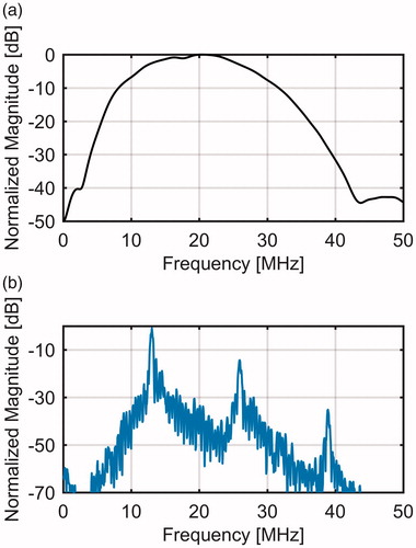
A high-frequency ultrasound scanner (Vevo^® 770, FujiFilm VisualSonics Inc., Toronto, ON, Canada) with a wide-band single-element transducer (RMV-710B, 25-MHz center frequency, f-number 2.1, 15 mm focal length) was used to transmit pulse trains of 30-cycle length at 13 MHz with a focal positive peak pressure of approximately 3.9 MPa. The Vevo 770 is a commercial ultrasound system used for small animal imaging. The transmit pulse length of 30-cycle and transmit pulse-frequency of 13 MHz were chosen so that the second (26 MHz) and third (39 MHz) harmonics could be detected with a reasonable signal to noise ratio within the bandwidth of the transducer. Figure 1 shows the bandwidth of the transducer and the frequency spectrum of a typical RF echo line. For the bandwidth, a flat reflector was placed at the focus of the transducer and the reflected signal was measured when the transducer was excited by a single cycle pulse.

Figure 1. (a) Measured bandwidth of the RMV-710B transducer and (b) the frequency spectrum of a typical RF echo line through the gel phantom.

2-D RF frames were generated by the mechanical sector sweep of the single-element transducer. The transducer was placed on top of the phantom and it was coupled to the phantom using ultrasonic coupling gel (Aquasonic, Parker Labratories, Inc. Fairfield, NJ). A stainless steel needle was inserted in the gel phantom and hot water, at various temperatures, was circulated in the needle in order to increase the temperature of the phantom only locally around the needle. The needle had an outer diameter of 3 mm with 0.5 mm wall thickness. Hot water was pumped in the needle from a temperature-controlled water bath (Haake DC10, Thermo Electron Corp., Newington, NH) using a peristaltic pump (Masterflex^® L/S^®, Cole Parmer, Chicago, IL). Temperature was recorded using a home-made calibrated needle type-K thermocouple and a digital thermometer (Omegaette HH306, Omega Eng. Inc., Stamford, CT). The thermocouple was made from a 125 micron nickel-chromium and a 125 micron nickel-alumel wire (California Fine Wire, Grover City, CA). The junction was made using an in-house constructed capacitive discharge welder. The completed thermocouple junction was fed inside a stainless-steel Precision Glide hypodermic needle (Becton-Dickinson, Franklin Lakes, NJ) from which the hub has been removed. The junction was glued inside the needle at the start of the bevel. The needles used were 23 gauge with a length of 38 mm. The 75-cm long wires were fed through a small diameter plastic tube (to prevent kinking of the wires) until the hubless end of the needle can be glued inside the plastic tube. The other end of the tube and wires are connected to a Type K miniature thermocouple plug from Omega Engineering.

The needle was placed laterally 2 mm away from the imaging plane of the transducer in order to minimize the RF signal distortion and/or saturation from the presence of the highly reflective metal needle. Figure 2 shows the schematic of the experimental setup and the needle position. The thermocouple was inserted in the sample, at the same depth as the heating needle. The tip of the thermocouple was placed within the imaging plane (2 mm away from the heating needle). The temperature at the thermocouple location was gradually increased from 26 °C to 46 °C. The tip of the thermocouple (which is within the imaging plane), and therefore the focal region of the transducer experienced the highest temperature rise from the needle at 2 mm due to the cylindrically symmetric temperature distribution.

Figure 2. Schematic of the experimental setup. The side view of the setup shows that the hot needle is placed laterally 2 mm away from the imaging plane of the transducer and the tip of the thermocouple is placed within the imaging plane (2 mm away from the heating needle). The temperature at the thermocouple location changed from 26 °C to 46 °C.

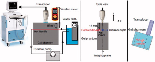
In this study, two sets of experiments were performed in each sample. In the first set, data collection was performed while the temperature was increasing from 26 to 46 °C by pumping hot water through the needle. The pump was also served as a source of motion to vibrate the phantom. Data collection was performed for the second time while the temperature was cooled down when the water bath and the peristaltic pump were turned off to eliminate vibrations in the phantom. The frequency of the induced vibration was estimated from the ultrasound M-mode data collected using the same transducer during the experiment. However, the M-mode data could not provide reliable estimation of displacement values along x and y directions as it is mostly sensitive to motion only in the ultrasound wave propagation direction (z direction). A calibrated vibration meter (GM63B, BENETECH, China) capable of measuring displacements in three dimensions within a range of 0.001 to 1.999 mm, was used to measure the vibration displacement in the heating needle entry location into the sample (shown in Figure 1) along x, y and z directions. The experiments were repeated 5 times in two different samples of the tissue-mimicking gel phantoms of the same composition and two different samples of ex vivo bovine muscle tissues for both set of experiments (with and without the presence of vibration in the sample).

The backscattered energies of the harmonics were obtained by first filtering the RF signal. Three band pass equiripple Finite Impulse Response (FIR) filters were designed to pass frequencies between 9 MHz to 16 MHz, 23 MHz to 29 MHz and 36 MHz to 42 MHz in order to separate the fundamental frequency, the second and the third harmonics content of the RF signal, respectively. The envelope of the signal was generated using the Hilbert transform. Envelope values were squared to calculate the backscattered energy at each data point on the RF signal. More details can be found in ref [31].

The change in the backscattered energy of each harmonic (CBE_i) at each temperature (T) and each pixel (x, y) was obtained by: (2) $${\mathit{CBE}}_i(x,y,T)=\frac{{\mathit{BE}}_i\left(x,y,T\right)-{\mathit{BE}}_i\left(x,y,\mathrm{ }26°\mathrm{C}\right)}{{\mathit{BE}}_i\left(x,\mathrm{ }y,\mathrm{ }26°\mathrm{C}\right)}\times 100.$$(2)

The conventional echo shift technique was performed by taking cross-correlation between two consecutive frames obtained at each temperature with a window size of 1×τ i.e., 0.077 μs (118 μm), and an overlap of 50%. 2 D gradient maps were obtained by differentiating the cumulative echo shifts along the axial direction [22].

The spatial resolution of ultrasound imaging transducer is commonly consisted of axial and lateral resolutions. In an ideal situation, i.e. in the absence of any noise or artifact that could affect the spatial resolutions, and with the assumption of a linear wave propagation, the highest theoretically attainable axial resolution in our method is equal to half the length of the transmit pulse, i.e. 30 × λ/2 = 1.8 mm [32]. The highest theoretically attainable lateral resolution in our method is equal to 1.22 × λ × f-number = 0.3 mm, which is derived from the geometry of the focused transducer used in our study [32]. The spatial resolution of the CBE technique in our study can therefore be assumed to be the same as the above-mentioned imaging resolution.

The B-mode images of the gel phantom and ex vivo bovine muscle tissue were also derived and presented for four different temperatures. The B-mode images were obtained using $20\mathrm{ }\times \log 10\left(\mathit{abs}(\mathit{hilbert}(\mathit{RFData}\right)))$ and displayed within the range of −80 to 0 dB using MATLAB (MathWorks, Natick, MA) where log10 is the common logarithm and abs is the absolute value.

Contrast to Noise Ratio (CNR) and Signal to Noise Ratio (SNR) were calculated as metrics in order to compare the image qualities of temperature maps between the two techniques and for the results of each technique in the presence and absence of vibration. CNR and SNR were calculated using [32]: (3) $$\mathit{CNR}=\frac{‖{\mu }_{\mathit{heated}}-{\mu }_{\mathit{unheated}}‖}{\sqrt{{\sigma }_{\mathit{heated}}^2+{\sigma }_{\mathit{unheated}}^2}}\mathrm{ },$$(3) (4) $$\mathit{SNR}=\frac{{\mu }_{\mathit{heated}}}{{\sigma }_{\mathit{heated}}},$$(4) where ${\mu }_{\mathit{heated}}$ and ${\mu }_{\mathit{unheated}}$ are the mean pixel values inside and outside the heated regions, respectively, and ${\sigma }_{\mathit{heated}}$ and ${\sigma }_{\mathit{unheated}}$ are the standard deviation of pixel values inside and outside the heated regions, respectively.

Results

B-mode images of the gel phantom and tissue sample are presented in Figure 3. Figures 4, 5, 7 and 8 show 2 D maps of change in backscattered energies of the acoustic harmonics (CBE₁, CBE₂ and CBE₃) in the tissue mimicking gel phantom and ex vivo tissue when the temperature was changed from 26 °C to 46 °C. Figures 6 and 9 show the gradient maps using the conventional echo-shift technique in the gel phantom and ex vivo tissue. The temperatures measured in the center of heated region within the imaging plane by the thermocouple were 31, 38, 42 and 46 °C as denoted in the figures. The vibration meter measured maximum displacement of 1.455, 0.221 and 1.030 mm in x, y and z directions. However, since the location where the vibration was measured was outside the sample, the amplitude of the measured vibration was presumably larger than what it was inside the sample. The frequency of the vibration was approximately 0.8 Hz. Tables 1 represents the SNR and CNR in CBE and gradient maps of Figures 4 to 9. The regions of interest for calculating the mean and the standard deviation inside and outside the heated areas were selected as horizontal rectangles as shown in Figures 4, 6, 7 and 9.

Figure 3. B-mode images of (left) tissue mimicking gel phantom and (right) ex vivo bovine muscle tissue. The temperatures measured by the inserted thermocouple were 31, 38, 42 and 46 °C at the center of heated region.

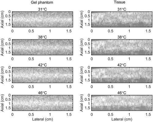
Figure 4. 2 D maps of CBE₁ (left), CBE₂ (middle), and CBE₃ (right) in tissue mimicking gel phantom while the temperature was cooling down from 46 °C to 26 °C and no vibration was present in the phantom. The temperatures measured by the inserted thermocouple were 31, 38, 42 and 46 °C at the center of heated region. The color bars represent percentage change in backscattered energy. The horizontal rectangles are the regions of interest for calculating the CNR and SNR.

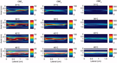
Figure 5. 2 D maps of CBE₁ (left), CBE₂ (middle), and CBE₃ (right) in tissue mimicking gel phantom while the temperature was elevated from 26 to 46 °C with the presence of vibration in the phantom. The temperatures measured by the inserted thermocouple were 31, 38, 42 and 46 °C at the center of heated region. The color bars represent percentage change in backscattered energy. The heated region is along the arrow in the lower right panel.

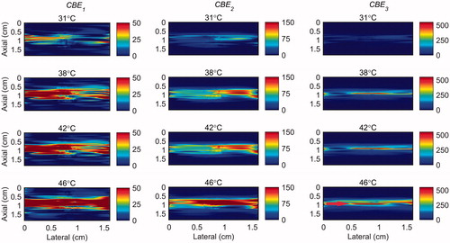
Figure 6. 2 D gradient maps in tissue mimicking gel phantom obtained using the conventional echo-shift technique without (left) and with (right) presence of vibration in the phantom. The temperatures measured by the inserted thermocouple were 31, 38, 42 and 46 °C at the center of heated region. The color bars represent the axial gradient of the cumulative time shifts in units of s/m. The horizontal rectangles are the regions of interest for calculating the CNR and SNR.

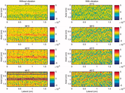
Table 1. The mean and the standard deviation of calculated SNR and CNR values for CBE and gradient maps with and without the presence of vibration in the gel phantom and tissue samples.

	Gel phantom		Tissue samples
	SNR	CNR	SNR	CNR
CBE1 (no-vib.)	1.91 ± 0.24	1.78 ± 0.24	3.1 ± 0.16	3.1 ± 0.16
CBE2 (no-vib.)	2.1 ± 0.62	2.08 ± 0.62	3.6 ± 0.55	3.6 ± 0.55
CBE3 (no-vib.)	2.68 ± 1.04	2.6 ± 0.99	3 ± 0.34	3 ± 0.34
Echo-shift (no-vib.)	1.71 ± 0.54	0.75 ± 0.12	0.61 ± 0.14	0.91 ± 0.2
CBE1 (vib.)	1.55 ± 0.55	1.48 ± 0.54	2.5 ± 0.15	2.5 ± 0.13
CBE2 (vib.)	2.09 ± 0.67	2.07 ± 0.67	2.3 ± 0.18	2.3 ± 0.18
CBE3 (vib.)	2 ± 0.85	1.98 ± 0.81	2 ± 0.21	2 ± 0.21
Echo-shift (vib.)	0.34 ± 0.3	0.09 ± 0.02	0.05 ± 0.03	0.08 ± 0.05

Discussion

Figures 4, 5, 7 and 8 show that the change in backscatter energy of acoustic harmonics are detectable in a sample where only a localized volume is heated. The results also show that this technique is nearly unaffected by the vibration induced in the sample. However, the CBE maps show that the backscatter energy of the harmonics were not consistently increasing with the temperature only in the heated region, especially in CBE₁. The variability was reduced by using higher harmonics (CBE₂ and CBE₃). Figures 4, 5, 7 and 8 also demonstrate that higher harmonics have higher sensitivity to temperature which is in agreement with our previous findings [31].

Figure 7. 2 D maps of CBE₁ (left), CBE₂ (middle), and CBE₃ (right) in ex vivo bovine muscle tissue while the temperature was cooling down from 46 °C to 26 °C and no vibration was present in the tissue. The temperatures measured by the inserted thermocouple were 31, 38, 42 and 46 °C at the center of heated region. The color bars represent percentage change in backscattered energy. The horizontal rectangles are the regions of interest for calculating the CNR and SNR.

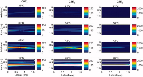
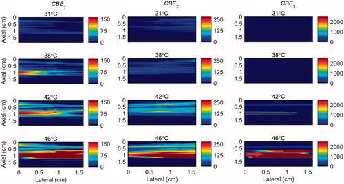
Figure 8. 2 D maps of CBE₁ (left), CBE₂ (middle), and CBE₃ (right) in ex vivo bovine muscle tissue while the temperature was elevated from 26 to 46 °C with the presence of vibration in the tissue. The temperatures measured by the inserted thermocouple were 31, 38, 42 and 46 °C at the center of heated region. The color bars represent percentage change in backscattered energy. The heated region is along the arrow in the lower right panel.

Figures 6 and 9 demonstrate that the gradient map obtained using the conventional echo-shift technique shows the heated region in the sample only in the case where the measurement was not affected by vibrations. However, it is important to note that there has been no motion compensation technique applied for obtaining these maps. It is anticipated that applying a motion compensation technique along with a very high-frame-rate data acquisition [24,33] will reduce the effect of motion artifacts in both methods.

Figure 9. 2 D gradient maps in ex vivo bovine muscle tissue obtained using the conventional echo-shift technique without (left) and with (right) presence of vibration in the tissue. The temperatures measured by the inserted thermocouple were 31, 38, 42 and 46 °C at the center of heated region. The color bars represent the axial gradient of the cumulative time shifts in units of s/m. The horizontal rectangles are the regions of interest for calculating the CNR and SNR.

The results in Table 1 show that the SNR and the CNR are higher in the images obtained using the nonlinear ultrasound technique compared to the ones using the echo-shift technique. The SNR and CNR values were significantly reduced in the image obtained using the echo-shift technique in the presence of vibration in the sample, compared to the one without vibration. The mean SNR was reduced by a factor of 5 from 1.71 to 0.34 and the mean CNR was reduced by a factor of 8.3 from 0.75 to 0.09 in the presence of phantom vibration. However, the SNR and CNR values in images obtained using the CBE₁, CBE₂, and CBE₃ reduced by approximately 0.81, 0.9 and 0.74 times in the phantom with vibration compared to the one without. The harmonics-based method is less sensitive to motion, since this technique does not depend on the correlation between consecutive RF frames. On the other hand, the performance of the echo-shift technique strongly depends on the correlation of the signals, which is directly affected by motion.

The magnitude of human organ motion depends on anatomical site. The motion induced in the samples is smaller than the motion of internal organs such as liver, kidney and pancreas due to normal breathing conditions [34]. However, the magnitude of the motion is comparable to that of such organs in forced breath holding condition and the frequency of the motion is similar to the heart rate [34].

The average and standard deviation of CBE₁, CBE₂ and CBE₃ values in the focal region were calculated in five trials with two tissue-mimicking gel phantoms and two ex vivo bovine muscle tissues at each temperature and shown in Figure 10. Tables 2 and 3 shows the standard deviation (SD) in the values of CBE_i in a randomly selected one trial and all the trials. This was done in order to show the sensitivity of the harmonics to temperature change. They also show the variation and consistency of the CBEs in one and multiple trials and different samples. The results show that the harmonics monotonically increase with temperature with a higher sensitivity at higher harmonics. CBE values are more consistent in the gel phantom compared to tissue samples. This could be due to higher variation in tissue samples compared to gel phantoms and lower SNR in tissue samples due to their higher attenuation. Higher harmonics in general show higher variation due to the lower SNR at higher harmonics.

Figure 10. The mean and standard deviation of CBE₁, CBE₂ and CBE₃ in (a) tissue-mimicking gel phantoms and (b) ex vivo bovine muscle tissues as a function of temperature. The error bars represent the standard deviation in five trials with two samples of tissue and gel phantoms.

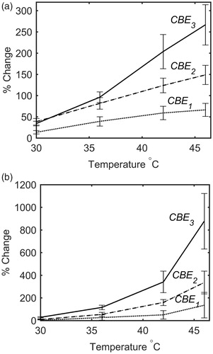
Table 2. The standard deviation of CBE₁, CBE₂ and CBE₃ in (left) one and (right) five trials with two tissue-mimicking gel phantoms of the same composition at three temperatures.

	One			All
	36°	42°	46°	36°	42°	46°
CBE1	±7	±10	±14	±10	±15	±15
CBE2	±7	±12	±18	±13	±17	±22
CBE3	±19	±44	±52	±12	±35	±47

Table 3. The standard deviation of CBE₁, CBE₂ and CBE₃ in (left) one and (right) five trials with two different ex vivo bovine muscle tissues at three temperatures.

	One			All
	36°	42°	46°	36°	42°	46°
CBE1	±18	±32	±62	±20	±31	±96
CBE2	±11	±14	±56	±18	±27	±90
CBE3	±23	±87	±148	±19	±95	±215

The standard error (SE) and the sensitivity (gradient) of measured CBE_i as a function of temperature (∂CBE_i/∂T) could represent the accuracy of temperature estimation of this technique. Lower SE values and higher sensitivity in the measured CBE_i lead to higher accuracy in temperature prediction. In order to estimate the accuracy of temperature prediction of this technique in ex vivo tissue samples, the mean and standard error ($\mathrm{SE}=\mathrm{SD}/\sqrt{5}$) of the measured CBE_i values were calculated and plotted as a function of temperature. Table 4 shows the lower and upper temperature band corresponding to the mean minus SE and mean plus SE of CBE_i values, respectively. Figure 11 demonstrates how the temperature ranges were obtained from the mean and SE of CBE_i. The results of Table 4 show that, in our study, the CBE₁ has the lowest accuracy that can roughly be estimated as ±3°, whereas the CBE₂ and CBE₃ have higher accuracies that can roughly be estimated as ±1°.

Figure 11. The mean and standard error of CBE₁, CBE₂ and CBE₃ in ex vivo bovine muscle tissues as a function of temperature. The error bars represent the standard error in five trials. The red and blue lines represent the lower and upper temperature band, respectively.

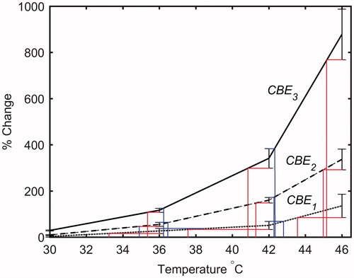
Table 4. The temperature range corresponding to mean minus SE and mean plus SE of CBE₁, CBE₂ and CBE₃ in ex vivo bovine muscle tissues at three measured temperatures.

	CBE1	CBE2	CBE3
46°	(43.6°, NA)	(45.2°, NA)	(45.2, NA)
42°	(37.7°, 42.8°)	(41.3°, 42.3)	(40.85, 42.3)
36°	(33.3°, 38.7°)	(34.9°, 36.5°)	(35.4, 36.2)

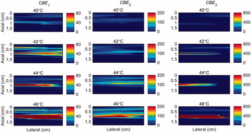
The temperature range used in this study was from 26 °C to 46 °C which was based on our previous work [31]. However in hyperthermia the tissue temperature increases from 37 to 45 °C. Therefore, in order to show the sensitivity of harmonics within this more relevant clinical temperature range, the maps of CBE₁, CBE₂ and CBE₃ in the gel phantom and tissue sample were plotted in Figures 12 and 13 in which the base level temperature was set to 38 °C and the temperature increases to 46 °C.

Figure 12. 2 D maps of CBE₁ (left), CBE₂ (middle), and CBE₃ (right) in tissue mimicking gel phantom while the temperature was elevated from 38 to 46 °C. The temperatures measured by the inserted thermocouple were 40, 42, 44 and 46 °C at the center of heated region. The color bars represent percentage change in backscattered energy (with a 38 °C baseline).

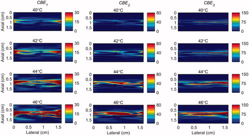
Figure 13. 2 D maps of CBE₁ (left), CBE₂ (middle), and CBE₃ (right) in ex vivo bovine muscle tissue while the temperature was elevated from 38 to 46 °C. The temperatures measured by the inserted thermocouple were 40, 42, 44 and 46 °C at the center of heated region. The color bars represent percentage change in backscattered energy (with a 38 °C baseline).

In this study, the change in harmonics occurred only due to temperature change at a constant source pressure in a homogenous gel phantom and tissue sample. The characteristics of a nonlinear field depend on the source pressure amplitude and the medium’s acoustic parameters (absorption coefficient, coefficient of nonlinearity and sound speed). Varying the source pressure amplitude and the presence of tissue heterogeneities (especially fat) will lead to some changes in amount of harmonic generation at different temperatures. An extension of this work will be to investigate the effect of source pressure amplitude on harmonics generation with varying temperature in a more heterogeneous medium.

In this study, 2^nd and 3^rd harmonics were generated and detected with a commercial high frequency ultrasound scanner used for small animal imaging. Our goal is to develop a noninvasive thermometry technique to be used during hyperthermia treatments on small animals such as mice [35], and/or in certain clinical applications such skin cancer treatment. In addition to that, higher transmit frequency enhances the generation of harmonics and increases the temperature dependence of acoustic harmonics generated [19, 21]. However, short focal length of the transducer and the relatively high transmit frequency limits the penetration depth of the ultrasound beam. The possibility of implementing this technique on transducers with lower transmit frequencies and longer focal lengths needs to be investigated. This, on the other hand, will reduce the spatial resolution of the ultrasound image and therefore, the gradient and the CBE maps. Moreover, harmonic generation will be a challenge at low frequencies (≈ 1 MHz). Therefore, mid-range frequencies (≈ 8 MHz) can potentially be more suitable for clinical thermometry. In addition to imaging and thermometry, in this study, locally heating the sample was done by circulating hot water inside a stainless steel needle. In addition, locally heated temperature maps can potentially be obtained from the CBE maps using calibration maps that convert the measured change in harmonics to the temperature change. Since harmonic generation in a given type of tissue depends on acoustic properties of the tissue, the characteristics of the transmit signal, heating pattern and the beam propagating path, the calibration experimental conditions should be as similar as possible to the measurements of interest. The accuracy and precision of temperature estimation using this technique can then be investigated. Our future studies will include generating temperature maps using a focused therapeutic ultrasound transducer as a heating modality which is more practical for clinical hyperthermia.

Conclusion

The results obtained in this study indicate that the change in backscatter energy of acoustic harmonics are detectable in a tissue-mimicking gel phantom and ex vivo bovine muscle tissues where only localized volumes were heated. In the absence of vibration in the sample, 2 D CBE and gradient maps were obtained using the harmonics and the RF echo-shift technique. In the presence of the vibration that is mechanically induced in the sample and without applying any motion compensation technique, identifying the heated region was feasible only by using the proposed method based on backscattered energies of the harmonics. It is anticipated that by incorporating an appropriate motion compensation technique, the performances of both methods will be improved.

Acknowledgements

The authors would like to acknowledge the technical assistance of Arthur Worthington from Dept. of Physics, Ryerson University, Toronto, Canada. This work was partially funded by the Ontario Research Fund– Research Excellence (ORF-RE) grant and the Natural Sciences and Engineering Research Council of Canada (NSERC Discovery grants) that were awarded to J. Tavakkoli and M. C. Kolios. Funding to purchase the equipment was provided by the Canada Foundation for Innovation, the Ontario Ministry of Research and Innovation, the Canada Research Chairs Program, and the Ryerson University Research Fund.

Disclosure statement

No potential conflict of interest was reported by the authors.

References

- Lewis MA, Staruch RM, Chopra R. Thermometry and ablation monitoring with ultrasound. Int J Hyperthermia. 2015;31(2):163–181.
- Arthur RM, Straube WL, Trobaugh JW, et al. Non-invasive estimation of hyperthermia temperatures with ultrasound. Int J Hyperthermia. 2005;21(6):589–600.
- Winter L, Oberacker E, Paul K, et al. Magnetic resonance thermometry: methodology, pitfalls and practical solutions. Int J Hyperthermia. 2016;32(1):63–75.
- Hynynen K. MRI-guided focused ultrasound treatments. Ultrasonics. 2010;50(2):221–229.
- Kim Y. Advances in MR image-guided high-intensity focused ultrasound therapy. Int J Hyperthermia. 2015;31(3):225–232.
- Rieke V, Pauly KB. MR thermometry. J Magn Reson Imaging. 2008;27(2):376–390.
- Field SB, Hand JW. An introduction to the practical aspects of clinical hyperthermia. London: Taylor and Francis, 1990.
- van der Zee J. Heating the patient: a promising approach? Ann Oncol. 2002;13(8):1173–1184.
- Dewhirst MW, Stauffer PR, Das S, et al. Chapter-21—Hyperthermia. In Gunderson LL, Tepper JE, editors. Clinical radiation oncology. 4th ed. Philadelphia: Elsevier, 2015.
- Mallory M, Gogineni E, Jones GC, et al. Therapeutic hyperthermia: the old, the new, and the upcoming. Crit Rev Oncol Hematol. 2016;97:56–64.
- Datta NR, Ordonez SG, Gaipl US, et al. Local hyperthermia combined with radiotherapy and/or chemotherapy: recent advances and promises for the future. Cancer Treat Rev. 2015;41(9):742–753.
- Cihoric N, Tsikkinis A, van Rhoon G, et al. Hyperthermia-related clinical trials on cancer treatment within the ClinicalTrials.gov registry. Int J Hyperthermia. . 2015;31(6):609–614.
- Bakker A, Holman R, Rodrigues DB, et al. Analysis of clinical data to determine the minimum number of sensors required for adequate skin temperature monitoring of superficial hyperthermia treatments. Int J Hyperthermia. 2018;34(7):910–917.
- Schooneveldt G, Bakker A, Balidemaj E, et al. Thermal dosimetry for bladder hyperthermia treatment. An overview. Int J Hyperthermia. 2016;32(4):417–433.
- Paulides MM, Bakker JF, Linthorst M, et al. The clinical feasibility of deep hyperthermia treatment in the head and neck: new challenges for positioning and temperature measurement. Phys Med Biol. . 2010;55(9):2465–2480.
- Law WK, Frizzell LA, Dunn F. Determination of the nonlinearity parameter B/A of biological media. Ultrasound Med Biol. 1985;11(2):307–318.
- Cain CA. Ultrasonic reflection mode imaging of the nonlinear parameter B/A: I. A theoretical basis. J Acoust Soc Am. 1986;80(1):28–32.
- Zhang D, Gong X-F. Experimental investigation of the acoustic nonlinearity parameter tomography for excised pathological biological tissues. Ultrasound Med Biol. 1999;25(4):593–599.
- Van Sloun R, Demi L, Shan C, et al. Ultrasound coefficient of nonlinearity imaging. IEEE Trans Ultrason, Ferroelect, Freq Contr. 2015;62(7):1331–1341.
- Ueno S, Hashimoto M, Fukukita H, et al. Ultrasound thermometry in hyperthermia. Proc IEEE Ultrason Symp. 1990, pp. 1645–1652.
- Liu X, Gong X, Yin C, et al. Noninvasive estimation of temperature elevations in biological tissues using acoustic nonlinearity parameter imaging. Ultrasound Med Biol. 2008;34(3):414–424.
- Simon C, VanBaren P, Ebbini ES. Two-dimensional temperature estimation using diagnostic ultrasound. IEEE Trans Ultrason Ferroelectr Freq Control. 1998;45(4):1088–1099.
- Liu D, Ebbini ES. Real-time two-dimensional temperature imaging using ultrasound. IEEE Trans Biomed Eng. 2010;57:12–16.
- Bayat M, Ballard JR, Ebbini ES. In vivo ultrasound thermography in presence of temperature heterogeneity and natural motions. IEEE Trans Biomed Eng. 2015;62(2):450–457.
- Arthur RM, Straube WL, Starman JD, et al. Noninvasive temperature estimation based on the energy of backscattered ultrasound. Med Phys. 2003;30(6):1021–1109.
- Arthur RM, Straube WL, Trobaugh JW, et al. In vivo change in ultrasonic backscattered energy with temperature in motion-compensated images. Int J Hyperthermia. 2008;24(5):389–398.
- Arthur RM, Basu D, Guo Y, et al. 3-D in vitro estimation of temperature using the change in backscattered ultrasonic energy. IEEE Trans Ultrason Ferroelectr Freq Control. 2010;57(8):1724–1733.
- Straube WL, Arthur RM. Theoretical estimation of the temperature dependence of backscattered ultrasonic power for noninvasive thermometry. Ultrasound Med Biol. 1994;20(9):915–922.
- van Dongen KWA, Verweij MD. A feasibility study for non-invasive thermometry using non-linear ultrasound. Int J Hyperthermia. 2011;27(6):612–624.
- Maraghechi B, Hasani MH, Kolios MC, et al. Temperature dependence of acoustic harmonics generated by nonlinear ultrasound wave propagation in water at various frequencies. J Acoust Soc Am. 2016;139(5):2475–2481.
- Maraghechi B, Kolios MC, Tavakkoli J. Temperature dependence of nonlinear acoustic harmonics in ex vivo tissue and tissue-mimicking phantom. Int J Hyperthermia. 2015;31(6):666–673.
- Cobbold RSC. Foundations of biomedical ultrasound. New York (NY): Oxford University Press; 2007.
- Foiret J, Ferrara KW. Spatial and temporal control of hyperthermia using real time ultrasonic thermal strain imaging with motion compensation, Phantom Study. PLoS One. 2015;10(8):e0134938–22.
- Langen KM, Jones DT. Organ motion and its management. Int J Radiat Oncol Biol Phys. 2001;50(1):265–278.
- Ernsting MJ, Worthington A, May JP, et al. Ultrasound drug targeting to tumors with thermosensitive liposomes. Proc IEEE Int Ultrason Symp. 2011;2011:1–4.