Mathematical modeling of the thermal effects of irreversible electroporation for in vitro, in vivo, and clinical use: a systematic review

Abstract

Introduction

Irreversible electroporation (IRE) is a relatively new ablation method for the treatment of unresectable cancers. Although the main mechanism of IRE is electric permeabilization of cell membranes, the question is to what extent thermal effects of IRE contribute to tissue ablation.

Aim

This systematic review reviews the mathematical models used to numerically simulate the heat-generating effects of IRE, and uses the obtained data to assess the degree of mild-hyperthermic (temperatures between 40 °C and 50 °C) and thermally ablative (TA) effects (temperatures exceeding 50 °C) caused by IRE within the IRE-treated region (IRE-TR).

Methods

A systematic search was performed in medical and technical databases for original studies reporting on numerical simulations of IRE. Data on used equations, study design, tissue models, maximum temperature increase, and surface areas of IRE-TR, mild-hyperthermic, and ablative temperatures were extracted.

Results

Several identified models, including Laplace equation for calculation of electric field distribution, Pennes Bioheat Equation for heat transfer, and Arrhenius model for thermal damage, were applied on various electrode and tissue models. Median duration of combined mild-hyperthermic and TA effects is 20% of the treatment time. Based on the included studies, mild-hyperthermic temperatures occurred in 30% and temperatures ≥50 °C in 5% of the IRE-TR.

Conclusions

Simulation results in this review show that significant mild-hyperthermic effects occur in a large part of the IRE-TR, and direct thermal ablation in comparatively small regions. Future studies should aim to optimize clinical IRE protocols, maintaining a maximum irreversible permeabilized region with minimal TA effects.

Keywords:

• Irreversible electroporation
• mild hyperthermia
• numerical analysis
• simulation
• thermal ablation

1. Introduction

Irreversible electroporation (IRE) is a relatively new ablation modality for the treatment of unresectable cancers [1]. Contrary to contemporary ablation techniques such as radiofrequency ablation (RFA) and microwave ablation (MWA), IRE is proposed as a nonthermal ablation technique [2]. Instead, IRE uses ultra-short, high-voltage pulses between electrodes to induce an altered membrane potential, which leads to the irreversible permeabilization of the membranes of tumor cells through the creation of nanopores [3]. These nanopores allow for increased transmembrane transport, which causes a disturbance in the cell’s homeostasis and consequent cell death through accidental and regulated cell death [4].

Since the proposed mechanism of IRE is nonthermal, the technique is supposedly less prone to a heat-sink effect, which is known to hamper the efficacy of RFA and MWA when performing ablations in the presence of large blood vessels [5]. Another possible advantage of IRE over thermal modalities includes the preservation of vital structures (e.g. blood vessels, bile ducts) traversing the ablation zones, since fibrous and collagen structures are typically not affected by IRE [6]. Therefore, the application of IRE is widely investigated for several indications, such as renal and prostate tumors [7,8], pancreatic cancer [9–12], and perihilar cholangiocarcinoma [10].

However, contrary to the current assumption that IRE is a nonthermal ablation modality, several studies do report on the presence of thermal ablative (TA) temperatures (T ≥ 50 °C) within the IRE ablation zones during treatment, with histological signs of thermal damage [13–16]. Moreover, it is presently unknown whether the reported hyperthermic effects of IRE, caused by slightly less elevated (mild-hyperthermic (MH)) temperatures 40 ≤ T [°C] < 50 [3,17–19], have a beneficial impact on the irreversible permeabilization effect (IPE; we chose IPE instead of IRE effect to distinguish between only the permeabilization effect, and the permeabilization and the thermal effects jointly produced by IRE), or could be seen as an unwanted side-effect. Potentially, temperature increase during IRE ablation might be needed to enhance the IPE and therefore contribute to a successful ablation [20]. On the other hand, IRE could cause thermal damage to vital structures if applied in the vicinity of thermally vulnerable structures. This leaves the true mechanism of work of IRE to be contentious.

Investigating the degree of mild-hyperthermic and thermally ablative effects in the IRE-treated region (IRE-TR) could provide more insight into the IRE process. Determination of these ratios in vivo or in clinical applications is challenging, since a limited amount of IRE settings and parameters can be explored. Simulations using mathematical models could therefore be very useful. In such simulations, the IRE settings and model parameters can be varied extensively, resulting in improvement of our understanding of the IRE mechanism.

Therefore, the aim of this systematic review is to summarize and review the mathematical models used to numerically simulate the heat-generating effect of IRE, and to assess the degree of mild-hyperthermic and thermally ablative effects of IRE in relation to the IRE-TR, as predicted by the simulation results provided by the studies that were included in this review. Accordingly, we investigated whether the analytical/numerical model calculations reported for IRE in the literature could be used to answer the following research questions:

• Does IRE produce a thermal elevation that results in mild-hyperthermic effects?

• Does IRE produce a thermal elevation that results in thermally ablative effects?

• What are the relative sizes expressed in percentages of the regions with the mild-hyperthermic and thermally ablative effects in the IRE-TR?

2. Methods

This systematic review was performed according to the Preferred Reporting Items for Systematic Reviews and Meta (PRISMA)-analyses guidelines [21,22]. In this article, the main data and equations were extracted, analyzed, and reviewed. Additional description of data or equations was added to Supplementary Appendices 1–6:

• Supplementary Appendix 1: Full description of the search strategies.

• Supplementary Appendix 2: Definitions of abbreviations, symbols, and extracted parameters.

• Supplementary Appendix 3: Extended mathematical description of IRE.

• Supplementary Appendix 4: Additional clarification of figures.

• Supplementary Appendix 5: Extended mathematical description applied to methods of analysis.

• Supplementary Appendix 6: Extended summary of study characteristics and results from included studies.

2.1. Study selection

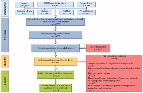
The medical and technical databases and search engines (Cochrane Library, Embase, IEEE Xplore Digital Library, PubMed, ScienceDirect, Scopus, and Web of Science) were searched for journal articles from inception up to and including 8 February 2019 using search terms related to ‘electroporation’, ‘mathematical models’, and ‘temperature’. A full description of the search strategy can be found in Supplementary Appendix 1. After removing the duplicates and excluding studies written in any other language than the English language, we searched for the terms ‘irreversible electroporation’ OR ‘ablation’ using EndNote X9, restricting the search terms to ‘Any Field’. Subsequently, the titles, the abstracts, and the full-text were screened for eligibility based on predefined inclusion and exclusion criteria that can be found in Sub section 2.2. Any disagreement was resolved by discussion between the review authors (PA) and (EvV). The flow diagram of the study selection is shown in Figure 1.

Figure 1. Flow diagram of the study selection.

2.2. Eligibility criteria

The focus of the studies is about IRE with rectangular pulses and a pulse length t_P ≥ 50 × 10⁻⁶ s. They must include analytical and/or numerical analysis of IRE and its heat-generating effect, performed in mammalian subject at macroscopic scale (i.e. tissue, scaffolds, cell suspension, phantoms including mammalian cell suspension). The inclusion criterion in the meta-analysis was the inclusion of a calculated temperature increase with the corresponding pulse parameters, and electrical and thermal properties of the target tissue. Studies that do not satisfy the criterion of the meta-analysis, or studies with the focus on the combination of IRE with other electroporation treatments (e.g. reversible electroporation, high-frequency IRE) or thermal ablations were included in qualitative synthesis.

Studies were excluded, if: (1) they exclude analytical and/or numerical analysis of the heat-generating effect of IRE, and the electrical properties of the target subject are not reported, (2) they applied IRE to nonmammalian subject, (3) they only include analytical and/or numerical analysis at microscopic scale (i.e. single cell, multiple cells, planar lipid membrane), (4) t_P <50 × 10⁻⁶ s or the IRE pulses are nonrectangular, (5) their focus related to general description of electroporation, pulses with low electric field strength, reversible electroporation (including agent/drug/gene delivery) or thermal ablation, (6) they are a review, (7) their focus is about design of pulse generator.

2.3. Data collection

Parameters and equations, which were used for the analytical and/or numerical analysis of IRE and its heat-generating effect, were extracted from studies included in qualitative synthesis. Data of the included studies were extracted by one author (PA) and checked by a second author (EvV). Any disagreement was resolved by discussion between the review authors. Abbreviations, parameters, quantities, and study characteristics extracted from the included studies were explained in Supplementary Appendix 2. The extracted equations were reviewed and summarized in Section 3 and extensively described in Supplementary Appendix 3. After explaining the analysis of certain study characteristics in Supplementary Appendix 5 (see Subsection 2.4), we summarized the extracted parameters and study characteristics in four tables that are shown in Supplementary Appendix 6.

2.4. Methods of analysis

2.4.1. Definitions of mild-hyperthermic and thermally ablative effects

Assuming the tissues to have an initial physiological temperature (T_init) of 37 °C and a thermally ablative threshold (T_th) of 50 °C (ΔT ≥ 13 °C), the following assumptions were made:

• The thermal elevation of 3 ≤ ΔT [°C] < 13 (40 ≤ T [°C] < 50) results in mild-hyperthermic effects.

• The thermal elevation of ΔT ≥ 13 °C (T ≥ 50 °C) results in thermally ablative effects.

• Accordingly, in the IRE-TR the relative sizes were calculated based on the regions with the thermal elevations of 3 ≤ ΔT [°C] < 13 for the mild-hyperthermic effects and ΔT ≥ 13 °C for the thermally ablative effects.

Please note that even though the value 50 °C may not instantaneously result in thermal damage, it was still chosen as a T_th. This because during IRE the duration of exposure to temperatures around 50 °C could be in the order of minutes [15,16], which is sufficiently long that thermal damage may indeed occur [14,23] and this is thus effectively a clinically relevant threshold value associated with a high likelihood of occurrence of thermal ablation.

2.4.2. Analysis of research questions

To answer the first two research questions, we extracted the maximum simulated temperature increase (ΔT_max [°C]) with the corresponding pulse parameters from studies included in meta-analysis. If the data extracted from the pulse parameters and/or the maximum simulated temperature was incomplete, the ΔT_max was not reported. In case of parametric study, in which ΔT_max was produced from several pulse parameters, the ΔT_max at the extreme ends of the figures were included.

For the third research question, if a study included 2D plots of electric field, and temperature distributions at the same position of the same model, then S_3ΔT13,Σ [m²], S_ΔT13,Σ [m²], and S_E-IRE(th),Σ [m²] were extracted, where S_3ΔT13,Σ is the total surface area of the simulated temperature increase within the range 3 ≤ ΔT [°C] < 13 that represents the region with mild-hyperthermic temperature increase, S_ΔT13,Σ is the total surface area of the simulated temperature increase with ΔT ≥ 13 °C that represents the thermally ablated region, and S_E-IRE(th),Σ is the total surface area of the simulated electric field with E ≥ E_IRE(th) that represents the IRE-TR, E [V⋅m⁻¹] is the magnitude of the electric-field strength and E_IRE(th) [V⋅m⁻¹] is the electric-field threshold of IRE; the minimum E required to ablate the target tissue. Even though E_IRE(th) was only used as a minimum required E to extract S_E-IRE(th),Σ for this analysis, it must be noticed that E_IRE(th) in reality also depends on pulse parameters (pulse voltage, pulse shape, pulse length, pulse number, and pulse frequency), temperature, and electrical conductivity of the target. It is also important to note that:

• the E_IRE(th) values correspond to the E_IRE(th) from the study from which S_E-IRE(th),Σ was extracted,

• the pulse parameters on which the values of ΔT_max, S_3ΔT13,Σ and S_ΔT13,Σ depend, are different for each study,

• in case of E_IRE(th) range, e.g. [E_IRE(th),1, E_IRE(th),2], the average of this range was used to calculate S_E-IRE(th),Σ. Specifically, E_IRE(th) = ½ (E_IRE(th),1 + E_IRE(th),2).

• if E_IRE(th) was not reported in a certain study, then the S_E-IRE(th),Σ was not calculated and, accordingly, included in the analysis.

The extraction of the surface areas was done excluding surface areas of the electrodes (S_elect [m²]). Using the software package ImageJ (National Institutes of Health, Bethesda, MD), we firstly imported the desired figure in ImageJ and assigned the pixels to distance ratio of the image using the known distance between the electrodes. Next, if the imported figure includes E- and ΔT-contours showing the conditions mentioned above, then we manually selected S_E [m²], S_ΔT [m²] and S_elect using the ‘Freehand selections’ tool; S_E is the selected surface area of the electric field strength and S_ΔT is the selected surface area of the temperature increase. In case of no contours, we used the ‘Threshold Color’ tool to set the threshold of the surface color to the minimum value mentioned above. Circular or rectangular electrodes were manually selected using ‘Oval selections’ tool, and ‘Rectangle’ tool. After the extraction, the ratios R_3ΔT13 [%] and R_ΔT13 [%] were calculated, where R_3ΔT13 is the ratio between the region with mild-hyperthermic temperature increase and IRE-TR, and R_ΔT13 is the ratio between the thermally ablated region and IRE-TR. The accurate description of the extracted surface areas and calculated ratios are shown in Supplementary Appendix 5.

2.5. Statistical analysis

Statistical analysis was applied to the data of the studies included in the meta-analysis to answer the three research questions. Specifically, we answered the first two research questions by calculating the median, the minimum, and the maximum of ΔT_max. For the third research question, the medians were calculated of R_3ΔT13, and R_ΔT13. The answers of all research questions were based on studies with experimentally applied pulse parameters. As an additional step, the linear regression was applied to model the relationship between S_E-IRE(th), R_3ΔT13 and R_ΔT13, and the energy density (u [J⋅m⁻³]; see Subsection 3.3.), ΔT_max, R_3ΔT13, and R_ΔT13.

2.6. Additional assumptions, definitions, methods of analysis, and notes

To preserve the continuous course, all remaining assumptions, definitions, methods of analysis, and notes were defined in Section 3 when the need arose.

3. Results

3.1. Study selection

After removal of duplicates and screening 3815 articles by title, abstract, and full-text, we included 58 articles [3,24–80] in the qualitative synthesis, and 26 articles [3,24–28,31,33,34, 36,37,39–44,48,49,55,59,60,64,66,73,80]) in the quantitative synthesis (meta-analysis and meta-regression). The full overview of the study selection is shown in Figure 1. The parameters extracted from the included studies are shown in Supplementary Appendix 6, with the definitions explained in Supplementary Appendix 2.

3.2. Review of mathematical description of IRE

In this section, we summarized and reviewed the mathematical equations used to describe the thermal behavior of IRE in multiple models with various types of model geometries, electrodes, pulse parameters, tissue properties, and boundary conditions. The extended description of the mathematical equations can be found in Supplementary Appendix 3. In addition, more details about the applied model parameters were included in Supplementary Appendix 6. In the included studies, the subjects were modeled in one-dimensional [25,30,50,64], two-dimensional [3,24,26–28,32–34,36–39,41,51–54,59,65,66,72,74,75,78], and/or three-dimensional space [26,29,31,35,40,42–49,55–58,60–63,67–71,73,77,79,80]. The calculations were performed analytically, or numerically using Finite Element Method or Finite Difference Method using the software packages e.g. CFdesign (Blue Ridge Numerics, Inc., Charlottesville, VA) [55], COMSOL Multiphysics (COMSOL AB, Stockholm, Sweden) [26,28,31,32,34–46,48,49,51–53,56–63, 65–67,70,71,73,74,76–78], FEMLAB (COMSOL AB, Stockholm, Sweden) [3,24,27], IRENA [79,81], Marc/Mentat (MSC Software Corp., Santa Ana, CA) [47,75], and QuickField (Terra Analysis, Denmark) [54]. Generally, numerical calculations were performed on three-dimensional subjects using the software package COMSOL Multiphysics, which uses Finite Element Method. Furthermore, an example of possible pulse sequence is shown in Figure 2. Here, V_P [V] is the electric potential (the voltage) of the pulses, t_P [s] is the duration of a single pulse, n_P [–] is the pulse number, N_P [–] is the total number of pulses, τ_P [s] is the duration between two pulses, and f_P [Hz] is the pulse frequency, which is calculated as (1) $${\mathrm{f}}_{\mathrm{P}}=\frac{1}{{\mathrm{t}}_{\mathrm{P}}+{\mathrm{\tau }}_{\mathrm{P}}}$$(1)

Figure 2. Overview of IRE pulses, with V_P [V] as the electric potential (the voltage) of the pulses, t_P [s] as the duration of a single pulse, n_P as the pulse number, N_P as the total number of pulses, τ_P [s] as the duration between two pulses, and f_P [Hz] as the pulse frequency.

For convenience, overview of definitions, symbols, and mathematical notations were summarized in Supplementary Appendix 2.

3.2.1. Electric-field distribution

3.2.1.1. Electric-potential models

The IRE can be mathematically described at macroscopic scale by calculating the electric-field [3,24,26–29,31,33,34,36–48,50–59,61–63,65,66, 68–70,72–75,78–80], and temperature distribution [3,24, 26–31,33,34,36,37,39–44,48,53,55,58,59,61,62,64,66,70,73,76,80] in a volume of a certain medium (e.g. tissue). This description starts with the calculation of the electric-potential distribution, which is obtained by simplifying the combination of Maxwell’s equations: Faraday’s law of induction and Ampère’s law, into the steady-state form (2) $$\nabla ·\left(\mathrm{\sigma }\nabla \mathrm{\Phi }\right)=0$$(2) where ∇ ⋅ [m⁻¹] is the divergence, σ [S⋅m⁻¹] is the electrical conductivity, ∇ [m⁻¹] is the gradient and Φ [V] is the scalar electric potential [3,24,26,27,29,31,33,34,36–48,50–59,62,63, 65,66,68–70,75,78–80]. Here, the vector quantities are expressed in bold and italic, while the scalar quantities have remained unchanged. Furthermore, the electrical conductivity of a medium can be assumed to be homogeneous, heterogeneous, isotropic, anisotropic, linear, and/or nonlinear (see Supplementary Appendix 2 Table A2.2 for the definitions of the medium properties and Supplementary Appendix 3 for extended description of medium properties). This electrical model can be used when several media are modeled with various electrical characteristics, such as cancerous tissue in a healthy tissue model, and tissue that includes blood vessels and nerves. Also, it is possible to choose a volume with homogenous, isotropic, and linear medium properties for simplicity. In this case, we can remove the electrical-conductivity term from Equation (2)(2) $$\nabla ·\left(\mathrm{\sigma }\nabla \mathrm{\Phi }\right)=0$$(2) and transform it into the Laplace’s equation (3) $${\nabla }^2\mathrm{\Phi }=0$$(3) with ∇² [m⁻²] as Laplace operator.

3.2.1.2. Electric-field model and threshold

For both Equations 2(2) $$\nabla ·\left(\mathrm{\sigma }\nabla \mathrm{\Phi }\right)=0$$(2) and 3(3) $${\nabla }^2\mathrm{\Phi }=0$$(3) , the calculated electric-potential distribution is used to determine the electric-field distribution in the volume of the medium using (4) $$\mathit{E}=-\nabla \mathrm{\Phi }$$(4) with E [V⋅m⁻¹] as the electric field [26,43,68,72,74,79,80]. Assuming the volume of the medium to be an arbitrary tissue, the electric-field distribution yields IRE when a minimum electric-field strength E_IRE(th) is obtained, providing the corresponding duration, number, shape, and the frequency of the pulses, and the tissue type. In Supplementary Appendix 6, a range of E_IRE(th) and its corresponding pulse parameters are shown for several tissue types. Additional details about the mathematical description of the electric-field component of IRE are shown in Supplementary Appendix 3.

3.2.1.3. Boundary conditions

For the calculation of the electric potential, a boundary condition (BC) needs to be applied to the boundaries between the electrodes (metallic part) and the media (BEM), and the boundaries at the outer surface (BOS) of the model. These boundaries could have a constant electric potential (Dirichlet BC; always applied by the included studies to BEM) [3,24,26–29,31–48,50–55,57–61, 64–66,68–76,78–80], zero electric current (Neumann BC; generally applied to BOS) [3,24,26,28,29,31–34,36–45,48,53, 57–61,66,69,70,73–75,78–80], or limited electric current to reduce the influence of the boundaries on the domain by virtually increasing the size of the domain while maintaining the number of nodes (Robin BC) [79]. See Figure 3.

Figure 3. Examples of applied boundary conditions for the calculations of the electric potential distribution with arrow representing electric-current flow through the outer surface of the model (I_BOS [A]). The red and the blue circles represent BEM with the electrodes given in the color gray, and black lines represent the BOS of the model. (A) shows Dirichlet boundary conditions at BEM and BOS, and (B) shows Dirichlet boundary conditions at BEM, and Neumann boundary conditions at BOS if I_BOS = 0 A or Robin boundary conditions if I_BOS is limited.

The preference of the boundary conditions depends on the type of the study. In case of active electrodes, obviously Dirichlet BC should be applied, while Neumann BC could be applied to the nonmetallic parts of the electrodes. For BOS, it is recommended to apply the Neumann BC for the clinical practice, since the simulated electric field can provide an upper limit to the temperature distribution [3].

3.2.2. Temperature distribution

3.2.2.1. Bioheat transfer models

Several heat transfer models were used for the calculation of thermal distributions (see Supplementary Appendix 3 for an extended summary). Nevertheless, the most utilized model is the Pennes bioheat equation (5) $$\mathrm{\rho }{\mathrm{c}}_{\mathrm{p}}\frac{\partial \mathrm{T}}{\partial \mathrm{t}}=\nabla \left(\mathrm{k}·\nabla \mathrm{T}\right)-{{\mathrm{\rho }}_{\mathrm{b}}{\mathrm{\omega }}_{\mathrm{b}}\mathrm{c}}_{\mathrm{b}}\left({\mathrm{T}-\mathrm{T}}_{\mathrm{art}}\right)+{\mathrm{Q}}_{\mathrm{m}}+\mathit{J}·\mathit{E}$$(5) where ρ [kg⋅m⁻³] is the mass density, c_p [J⋅kg⁻¹⋅°C⁻¹] is the specific heat capacity, T [°C] is the temperature, t [s] is the time, k [W⋅m⁻¹⋅°C⁻¹] is the thermal conductivity, c_b [J⋅kg⁻¹⋅°C⁻¹] is the specific heat capacity of the blood, ρ_b [kg⋅m⁻³] is the blood density, ω_b [s⁻¹] is the blood perfusion rate (blood perfusion w_b [kg⋅m⁻³⋅s⁻¹] = ρ_b ⋅ ω_b), T_art [°C] is the arterial blood temperature, Q_m [W⋅m⁻³] is the metabolic heat generation, and J · E [W⋅m⁻³] is the heat generation rate per unit volume (the Joule Heating) [3,24,26–29,31,33,34,36, 37,39,41–44,48,53,55,58,61,62,66,70,73,76,80]. Over the intrapulses of IRE, the Joule Heating term can be simplified into (6) $$\mathit{J}·\mathit{E}=\mathrm{\sigma }{\left|\mathit{E}\right|}^2$$(6) when IRE is used [3,24,26–29,33,34,36,40,41,44,48,53,55,58,59,66,76].

Even though the majority of the studies applied the Pennes bioheat model, the choice of a suitable heat transfer model depends on the modeling conditions. Yet, for the clinical practice the Pennes bioheat model is recommended due to its ability to calculate the temperature distribution in a domain with heterogeneous and nonlinear electrical and thermal characteristics, considering the metabolic heat generation and heat sink effect.

3.2.2.2. Boundary conditions

To calculate the thermal distribution, boundary conditions need to be applied to the BEM and BOS of the model. These boundaries could have a constant temperature (Dirichlet BC) [28,33,34,36,41,53,55], a limited heat flow (Robin BC) [25,29,30,37,40,43–45,59], or no heat flow at all (Neumann BC) [3,24,26,27,29,31,39,40,43,58, 61,73,80] (see Figure 4). As for the heat transfer models, the proper choice of the boundary conditions depends on the modeling conditions. Nevertheless, for the clinical practice the Neumann BC is recommended to both BEM and BOS to produce an upper limit to the temperature distribution [3].

Figure 4. Examples of applied boundary conditions for the calculations of the temperature distribution. The brown circles represent BEM with the electrodes given in the color gray, and black lines represent the BOS of the model. Arrows represent heat flux vector that is normal to the BEM (q_BEM [W⋅m⁻²]) and the BOS (q_BOS [W⋅m⁻²]). At both BEM and BOS (A) shows Dirichlet boundary conditions, and (B) shows Neumann boundary conditions if q_BEM = 0 W⋅m⁻² and q_BOS = 0 W⋅m⁻², or Robin boundary conditions if q_BEM and q_BOS are limited.

3.2.2.3. Estimation of time durations of mild-hyperthermic and thermally ablative temperatures

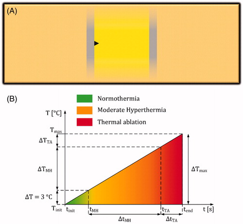
Time durations of mild-hyperthermic (Δt_MH) and thermally ablative (Δt_TA) temperatures as a function of time were generally absent in the included studies. Nevertheless, these durations are relevant and the values can be estimated by determining the ratios between the time durations of these effects and the total treatment time (N_P ⋅ (t_P + τ_P)) [s]. Even though different model properties with various electrode shapes were utilized by the included studies, for simplicity the ratios were calculated by assuming a homogeneous, isotropic, and linear model within two infinite plate electrodes to obtain a homogeneous electric-field strength (see Figure 5(A)). To further simplify the assumptions, the heat conduction, convection, and the metabolic heat generation were neglected within the plate electrodes, allowing the bioheat transfer equation to be simplified into (7) $$\mathrm{\Delta }\mathrm{T}=\frac{\mathit{J}·\mathit{E}·{\mathrm{t}}_{\mathrm{P}}·{\mathrm{f}}_{\mathrm{P}}}{\mathrm{\rho }{\mathrm{c}}_{\mathrm{p}}}\mathrm{\Delta }\mathrm{t}$$(7) where ΔT [°C] is the temperature increase during the time period Δt [s] and t_P · f_P is a dimensionless factor that averages the Joule Heating term over the entire intra- and interpulse duration (see Supplementary Appendix 3). For illustration, Figure 5(B) shows the temperature profile of Equation 7(7) $$\mathrm{\Delta }\mathrm{T}=\frac{\mathit{J}·\mathit{E}·{\mathrm{t}}_{\mathrm{P}}·{\mathrm{f}}_{\mathrm{P}}}{\mathrm{\rho }{\mathrm{c}}_{\mathrm{p}}}\mathrm{\Delta }\mathrm{t}$$(7) as a function of time over the period t_end – t_init (or N_P · (t_P + τ_P)) with normothermic (from t_init to t_MH), mild-hyperthermic (from t_MH to t_TA) and thermally ablative zones (from t_TA to t_end). According to this figure, the ratios can be calculated by (8) $${\mathrm{R}\mathrm{\Delta }\mathrm{t}}_{\mathrm{MH}}=\frac{\mathrm{\Delta }{\mathrm{t}}_{\mathrm{MH}}}{{\mathrm{N}}_{\mathrm{P}}\cdot ({\mathrm{t}}_{\mathrm{P}}+{\mathrm{\tau }}_{\mathrm{P}})}$$(8) and (9) $${\mathrm{R}\mathrm{\Delta }\mathrm{t}}_{\mathrm{TA}}=\frac{\mathrm{\Delta }{\mathrm{t}}_{\mathrm{TA}}}{{\mathrm{N}}_{\mathrm{P}}\cdot ({\mathrm{t}}_{\mathrm{P}}+{\mathrm{\tau }}_{\mathrm{P}})}$$(9) where RΔt_MH and RΔt_TA are dimensionless ratios between mild-hyperthermic and thermally ablative time durations, and the total treatment time. Duo to the linearity of Figure 5(B), (10) $$\frac{\text{Δt}}{{\mathrm{N}}_{\mathrm{P}}\cdot ({\mathrm{t}}_{\mathrm{P}}+{\mathrm{\tau }}_{\mathrm{P}})}=\frac{\text{ΔT}}{\mathrm{\Delta }{\mathrm{T}}_{\max }\mathrm{ }}$$(10)

Figure 5. (A) Assumed model that includes infinite electrode plates to calculate the temperature increase during IRE. The electrodes are presented as gray rectangles with infinite length and IRE-TR as a yellow rectangle. The black triangle represents a possible location in the model with maximum temperature increase. (B) An example of a temperature increase profile based on Equation 7(7) $$\mathrm{\Delta }\mathrm{T}=\frac{\mathit{J}·\mathit{E}·{\mathrm{t}}_{\mathrm{P}}·{\mathrm{f}}_{\mathrm{P}}}{\mathrm{\rho }{\mathrm{c}}_{\mathrm{p}}}\mathrm{\Delta }\mathrm{t}$$(7) , which is divided in normothermia (from t_init to t_MH), moderate hyperthermia (MH; from t_MH to t_TA), and thermal ablation (TA; from t_TA to t_end).

After combining Equations 8(8) $${\mathrm{R}\mathrm{\Delta }\mathrm{t}}_{\mathrm{MH}}=\frac{\mathrm{\Delta }{\mathrm{t}}_{\mathrm{MH}}}{{\mathrm{N}}_{\mathrm{P}}\cdot ({\mathrm{t}}_{\mathrm{P}}+{\mathrm{\tau }}_{\mathrm{P}})}$$(8) and 9(9) $${\mathrm{R}\mathrm{\Delta }\mathrm{t}}_{\mathrm{TA}}=\frac{\mathrm{\Delta }{\mathrm{t}}_{\mathrm{TA}}}{{\mathrm{N}}_{\mathrm{P}}\cdot ({\mathrm{t}}_{\mathrm{P}}+{\mathrm{\tau }}_{\mathrm{P}})}$$(9) with 10(10) $$\frac{\text{Δt}}{{\mathrm{N}}_{\mathrm{P}}\cdot ({\mathrm{t}}_{\mathrm{P}}+{\mathrm{\tau }}_{\mathrm{P}})}=\frac{\text{ΔT}}{\mathrm{\Delta }{\mathrm{T}}_{\max }\mathrm{ }}$$(10) , the time durations can be replaced by the temperature differences as follows (11) $${\text{RΔt}}_{\mathrm{MH}}=\frac{\mathrm{\Delta }{\mathrm{T}}_{\mathrm{MH}}}{\mathrm{\Delta }{\mathrm{T}}_{\max }\mathrm{ }}$$(11) with (12) $$\mathrm{\Delta }{\mathrm{T}}_{\mathrm{MH}}\in \left\{\begin{array}{c}\mathrm{\Delta }\mathrm{T}-3\\ 10\end{array}\mathrm{ }\begin{array}{c}3\le \mathrm{\Delta }\mathrm{T}<13\\ \mathrm{\Delta }\mathrm{T}\ge 13\end{array}\right.$$(12) and (13) $${\text{RΔt}}_{\mathrm{TA}}=\frac{\mathrm{\Delta }{\mathrm{T}}_{\mathrm{TA}}}{\mathrm{\Delta }{\mathrm{T}}_{\max }}$$(13) with (14) $$\mathrm{\Delta }{\mathrm{T}}_{\mathrm{TA}}\in \left\{\mathrm{\Delta }\mathrm{T}-13\mathrm{ }|\text{ ΔT}\ge 13\right\}$$(14)

Since the required data to calculate the total treatment time for each study are available, the calculation of RΔt_MH and RΔt_TA allows us to estimate the time durations of mild hyperthermia and thermal ablation using Equations 8(8) $${\mathrm{R}\mathrm{\Delta }\mathrm{t}}_{\mathrm{MH}}=\frac{\mathrm{\Delta }{\mathrm{t}}_{\mathrm{MH}}}{{\mathrm{N}}_{\mathrm{P}}\cdot ({\mathrm{t}}_{\mathrm{P}}+{\mathrm{\tau }}_{\mathrm{P}})}$$(8) and 9(9) $${\mathrm{R}\mathrm{\Delta }\mathrm{t}}_{\mathrm{TA}}=\frac{\mathrm{\Delta }{\mathrm{t}}_{\mathrm{TA}}}{{\mathrm{N}}_{\mathrm{P}}\cdot ({\mathrm{t}}_{\mathrm{P}}+{\mathrm{\tau }}_{\mathrm{P}})}$$(9) .

3.2.3. Thermal damage

Exposing biological cells or tissues to temperatures higher than their physiological temperatures for extended periods of time can result in thermal damage. In other words, irreversible changes in tissue structure or function that includes cell death, microvascular blood flow stasis, and/or protein coagulation processes [40]. The thermal damage starts at the mild-hyperthermic temperature 42 °C–43 °C with exposure period between several seconds to hours, depending on the temperature level [40,53,58]. In the case of relatively short exposure, damage is relatively limited up to 50 °C–60 °C, at which level the damage dramatically increases [40,58]. For instance, 73.4 °C is considered the threshold for instantaneous thermal damage in liver tissue that results in tissue whitening [53]. Nevertheless, 50 °C could be generally assumed as a typical and relevant threshold one should attempt to avoid in the clinic as when temperatures around 50 °C occur during IRE the duration of exposure to these elevated temperatures could be in order of minutes [15,16], with a significant likelihood of resulting in thermal damage [14,23]. Multiple studies quantified the amount of thermal damage using the Arrhenius equation [3,26,28,30,33,34,36, 40,41,53,55,58,59,80]. This equation is a first-order reaction rate constant that describes the rate of a chemical reaction. The Arrhenius equation, firstly applied by Henriques and Moritz in 1947 for skin burn analysis in pigs [18,82–84], uses Maxwell–Boltzmann statistics to describe the conversion of biological substances at temperature T_K(t) from a native state to a thermally damaged state at a rate constant (15) $$\frac{\partial \mathrm{\Omega }\left(\mathrm{t}\right)}{\partial \mathrm{t}}=\mathrm{A}\mathrm{ exp}\left(-\frac{{\mathrm{U}}_{\mathrm{a}}}{\dot{\mathrm{R}}{\mathrm{T}}_{\mathrm{K}}\left(\mathrm{t}\right)}\right)$$(15) where Ω(t) is the dimensionless time dependent accumulated thermal damage, A [s⁻¹] is the pre-exponential factor (or collision frequency), a measure for molecular collision frequency, U_a [J⋅mol⁻¹] is the activation energy required for the molecules to denature, Ṙ [J⋅mol⁻¹⋅K⁻¹] is the ideal gas constant (Ṙ = 8.314 [J⋅mol⁻¹⋅K⁻¹]), and T_K(t) [K] is the time-dependent absolute temperature [80]. Then, the thermal damage is calculated by integrating the Arrhenius Equation over a certain period of time, resulting in (16) $$\mathrm{\Omega }\left(\mathrm{t}\right)=\underset{{\mathrm{t}}_{\mathrm{init}}}{\overset{t}{\int }}\mathrm{A}\mathrm{ exp}\left(-\frac{{\mathrm{U}}_{\mathrm{a}}}{\dot{\mathrm{R}}{\mathrm{T}}_{\mathrm{K}}\left(\mathrm{t}\right)}\right)\mathrm{d}\mathrm{t}$$(16) where t_init [s] is the initial time point of the heating process [3,26,28,30,33,34,36,40,41,53,55,58,59,80]. The power of this analysis is to provide an estimation of the damaged fraction of a certain volume of a tissue constituent that is exposed to temperature T_K. This estimation is calculated by hypothetically expressing both the intact and damaged substances in (17) $$\mathrm{\Omega }\left(\mathrm{t}\right)=\ln \left(\frac{\mathrm{N}\left({\mathrm{t}}_{\mathrm{init}}\right)}{\mathrm{N}\left(\mathrm{t}\right)}\right)$$(17) where N(t_init) and N(t) represent the amount of the substances (expressed in number or concentration) in the tissue volume just before the temperature exposure and at time t [33,55,59]. Then, the probability of thermal damage (the estimation of the damaged fraction), Υ [%], in the volume of the tissue constituent is calculated [33,53,55,59,80] using (18) $$\mathrm{{\rm Y}}=100\left(1-\exp (-\mathrm{\Omega }\left(\mathrm{t}\right)\right)$$(18)

The severeness of injuries due to the heating process can be represented by a threshold Ω_th. For instance, it has been shown that the threshold for burn injuries in blood-perfused skin is Ω_th = 0.53 (Υ = 41%) while it increases to Ω_th = 10,000 (Υ = 100%) for third-degree burns [40,58]. In order to describe the thermal damage processes, such as cell death, microvascular blood flow stasis, or protein coagulation, suitable A, and U_a values must be chosen for each process, which are tissue specific and experimentally determined [53]. Examples of such values can be found in Supplementary Appendix 6.

Another approach to describe the thermal damage is to calculate the cumulative equivalent minutes at 43 °C (CEM43 °C [min]; also defined as the thermal isoeffect dose t₄₃ [min]) [25,26,29,31,58,76]. CEM43°C is a concept, introduced by Sapareto and Dewey [19], which scales the exposure time of a time-varying temperature to an equivalent exposure time at the reference temperature 43 °C. Specifically, during the equivalent exposure time the tissue is assumed to be constantly held at 43 °C. CEM43°C can be described as (19) $$\mathrm{CEM}43°\mathrm{C}={\int }_{{\mathrm{t}}_{\mathrm{init}}}^{{\mathrm{t}}_{}}{\mathrm{R}}^{43-{\mathrm{T}}_{\mathrm{d}t}}\mathrm{d}t$$(19) where T_dt is the average temperature over the time differential dt, R is the factor to compensate for a 1 °C temperature change with R = 0.25 when T_dt ≤ 43 °C and R = 0.5 when T_dt >43°C. In this case, the severeness of injuries due to the heating process can be represented by a threshold CEM43°C_(th). Examples of such values can be found in Supplementary Appendix 6 and [85,86].

The use of a suitable thermal damage model depends on both the temperature range to which the target had been exposed to, and the desired expression of the thermal damage outcome. E.g., CEM43°C can provide a reasonable prediction of cell death for the temperature range 40 °C–47 °C [87]. However, it does not provide the probability of thermal damage as in the Arrhenius equation. On the other hand, the Arrhenius equation may overestimate the cell death at the start of the mild-hyperthermic temperature range [88]. More information about both models can be found in [19,88,89].

3.2.4. Tissue properties

The electric-field and temperature distributions of IRE have been calculated for multiple tissue types. For example, IRE has been applied to artery [33,34,36,41], brain [31,40,57,66, 69,73], breast [28,29,35], cervix [78], eye [44], in vitro cell suspension [30,43,47,60,61,75], kidney [45,63,65], liver [3,24,37–39,46,48,53,54,62,71,72,74,76,77,79,80], pancreas [52,70], prostate [28,32,49,50,56,64,67,68], rectal wall [51], skin [25,58], small intestine [59], and subcutaneous tissue [42]. Although some studies used the same tissue type, often different tissue properties were applied, which were classified as homogeneous or heterogeneous, isotropic or anisotropic, and linear or nonlinear. The definitions of these terms can be found in Supplementary Appendix 2 Table A2.2. For instance, the tissue properties were generally assumed to be isotropic linear, e.g. σ, ρ, c_p, k, Q_m, w_b, A, and U_a. Specifically, this was the case for ρ, c_p, Q_m, w_b, A, and U_a in all of the included studies. However, some studies assumed isotropic nonlinear tissue properties, e.g. σ(E) [42,45,53,54,56,57,59,63,66,68–71, 77,79], σ(T) [3,40,43,45,60], σ(E,T) [31,37,40,45,62,73,76,80], σ(E, t) [46,78], and k(T) [3]. In particular, most of the studies fitted the electrical conductivity in the form (20) $$\mathrm{\sigma }\left(E\right)={\mathrm{\sigma }}_{\mathrm{init}}+\left({\mathrm{\sigma }}_{\max }-{\mathrm{\sigma }}_{\mathrm{init}}\right)\frac{1}{1+{\mathrm{a}}_1\exp \left(-\frac{\mathrm{E}-{\mathrm{a}}_2}{{\mathrm{a}}_3}\right)}$$(20) with (21) $${\mathrm{a}}_2=\frac{{\mathrm{E}}_{\mathrm{IRE}\left(\mathrm{th}\right)}+{\mathrm{E}}_{\mathrm{RE}\left(\mathrm{th}\right)}}{2}$$(21) and (22) $${\mathrm{a}}_3=\frac{{\mathrm{E}}_{\mathrm{IRE}\left(\mathrm{th}\right)}-{\mathrm{E}}_{\mathrm{RE}\left(\mathrm{th}\right)}}{{\mathrm{a}}_4}$$(22) where σ_init [S⋅m⁻¹] is the initial electrical conductivity of the target medium before application of IRE, σ_max [S⋅m⁻¹] is the electrical conductivity of the maximally permeabilized medium, and a₁ and a₄ are the sigmoid function parameters. Additional detail about nonlinear electrical conductivities is provided in Supplementary Appendix 3.

The majority of the included studies applied a static (constant) electrical conductivity to calculate the electric field distribution. However, as shown by [90,91] for example, the electrical conductivity has a dynamic behavior due to its increase during the electroporation. By including a dynamic electrical conductivity, the numerical models can be better correlated to the experimental data, such as the electric current, as shown by [63,92]. In addition, the inclusion of the dynamic behavior can reduce the variability of E_IRE(th) as was demonstrated by [63] in canine kidneys (575 × 10² ± 67 V⋅m⁻¹; versus 501 × 10² ± 121⋅10² V⋅m⁻¹ obtained from the model with statistic electrical conductivity) resulting in a proper prediction of E_IRE(th). An additional effect of the dynamically increasing electrical conductivity is the corresponding increase of the electric-field strength as was demonstrated by [63,68]. A larger electrical conductivity and electric-field strength result in a larger temperature increase (see Equations 5(5) $$\mathrm{\rho }{\mathrm{c}}_{\mathrm{p}}\frac{\partial \mathrm{T}}{\partial \mathrm{t}}=\nabla \left(\mathrm{k}·\nabla \mathrm{T}\right)-{{\mathrm{\rho }}_{\mathrm{b}}{\mathrm{\omega }}_{\mathrm{b}}\mathrm{c}}_{\mathrm{b}}\left({\mathrm{T}-\mathrm{T}}_{\mathrm{art}}\right)+{\mathrm{Q}}_{\mathrm{m}}+\mathit{J}·\mathit{E}$$(5) and 6(6) $$\mathit{J}·\mathit{E}=\mathrm{\sigma }{\left|\mathit{E}\right|}^2$$(6) ). To determine the thermal effects and to properly estimate the possible lesion size of the treatment, it is important to include the dynamic behavior of the electrical conductivity in the treatment planning.

3.3. Synthesis of data, meta-analysis, and meta-regression

This section summarizes the extracted data from the included studies, focusing on the maximum simulated temperature increase, and the energy density that was calculated as (23) $$\mathrm{u}={\mathrm{\sigma }}_{\mathrm{init}}{\left|\frac{{\mathrm{V}}_{\mathrm{P}}}{\mathrm{D}}\right|}^2{\mathrm{t}}_{\mathrm{P}}{\mathrm{N}}_{\mathrm{P}}$$(23) with u [J⋅m⁻³] as the energy density, and D [m] as the distance between electrodes (see Figure 6). Important: Please note that the u of an included study is not plotted if one of the extracted parameters in Equation 23(23) $$\mathrm{u}={\mathrm{\sigma }}_{\mathrm{init}}{\left|\frac{{\mathrm{V}}_{\mathrm{P}}}{\mathrm{D}}\right|}^2{\mathrm{t}}_{\mathrm{P}}{\mathrm{N}}_{\mathrm{P}}$$(23) is missing.

Figure 6. Examples of electrode configurations applied in studies to calculate the electric-field distribution, with the colors gray and brown as metallic and insulation parts, respectively. These configurations represent: (A) spherical electrodes, (B) needle and surface electrodes, (C) circular plate electrode enclosed by a ring electrode, (D, E) plate electrodes, (F) endovascular electrodes; contralateral electrodes have the same electric potential, (G) needle electrodes, (H) bipolar needle electrode; contralateral electrodes have different electric potential. In each configuration, the distances d [m] and D [m] were defined for the calculation of the energy density. Several studies assumed the needle and bipolar electrodes to be cylinders in 3D models. Other studies assumed the needle and spherical electrodes to be circles in 2D models.

3.3.1. Organ-dependent electrical and thermal properties

The calculations of ΔT_max, R_3ΔT13, R_ΔT13, and u are based on organ-dependent electrical and thermal characteristics, such as E_IRE(th), σ, and other properties provided in Equation 5(5) $$\mathrm{\rho }{\mathrm{c}}_{\mathrm{p}}\frac{\partial \mathrm{T}}{\partial \mathrm{t}}=\nabla \left(\mathrm{k}·\nabla \mathrm{T}\right)-{{\mathrm{\rho }}_{\mathrm{b}}{\mathrm{\omega }}_{\mathrm{b}}\mathrm{c}}_{\mathrm{b}}\left({\mathrm{T}-\mathrm{T}}_{\mathrm{art}}\right)+{\mathrm{Q}}_{\mathrm{m}}+\mathit{J}·\mathit{E}$$(5) . For these characteristics, a range of selected values was summarized in Table 1 and plotted in Figure 7 both for cancerous and healthy tissues. Please note that k_init [W⋅m⁻¹⋅°C⁻¹] represents the initial thermal conductivity before the start of the heating process. To repeat, the electrical and thermal characteristics extracted from the included studies are provided in Supplementary Appendix 6 Table A6.2. Additional electrical and thermal characteristics can be found in the IT’IS database for thermal and electromagnetic parameters of biological tissues [93].

Figure 7. Parameters of different tissue types, as selected by the included studies (Supplementary Appendix 6 – Table A6.2). For (A)–(E), red circles represent cancerous tissue and green diamonds represent healthy tissue. In all figures, brain tissue represents gray and white matter, skin tissue represents subcutaneous tissue, fat layer, dermis and stratum epidermis, eye tissue represents aqueous, cornea, lens, retina, sclera and vitreous, colon tissue represents both colon and rectal wall, blood vessel tissue represents artery, blood and blood vessel, and finally, muscle tissue represents muscles with longitudinal and transversal properties. The selected tissue properties in this figure show (A) the initial electrical conductivity (σ_init [S⋅m⁻¹]) before the application of IRE (the σ_init values that exceeded 1 S⋅m⁻¹ were 1.5 S⋅m⁻¹ for aqueous and vitreous in the eye [44], and 2.31 S⋅m⁻¹ for cancerous breast tissue [28]), (B) mass density (ρ [kg⋅m⁻³]), (C) specific heat capacity (c_p [J⋅kg⁻¹⋅°C⁻¹]), (D) initial thermal conductivity before the start of heating process (k_init [W⋅m⁻¹⋅°C⁻¹]), (E) blood perfusion (w_b [kg⋅m⁻³⋅s⁻¹]; the w_b value that exceeded 20 kg⋅m⁻³⋅s⁻¹ was 212 kg⋅m⁻³⋅s⁻¹ for both healthy and cancerous pancreas tissues [70]; if w_b could not be extracted nor calculated due to the absence of blood density (ρ_b [kg⋅m⁻³]), then w_b was calculated by assuming ρ_b = 1060 kg⋅m⁻³), and (F) Electric-field threshold of irreversible electroporation (E_IRE(th) [V⋅m⁻¹]) as function of pulse number. Please note that the y-axis in (F) can be read in [V⋅cm⁻¹], and that empty fields are present in (B)–(F) due to the lack of data.

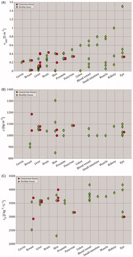
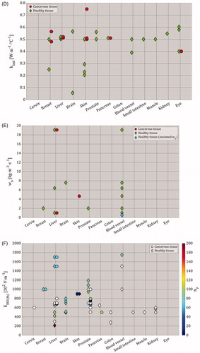
Table 1. Summary of organ-dependent electrical and thermal characteristics for cancerous and healthy tissues (see Supplementary Appendix 6 – Table A6.2).

Electrical and thermal properties	Cancerous tissue	Healthy tissue
Initial electric conductivity (σinit [S⋅m^−1])	[0.025, 0.435]^a	[0.01, 1]^b
Mass density (ρ [kg⋅m^−3])	[1000, 1186]	[850, 1305]
Specific heat capacity (cp [J⋅kg^−1⋅°C^−1])	[2926, 4000]	[2300, 4180]
Initial thermal conductivity (kinit [W⋅m^−1⋅°C^−1])	[0.4, 0.75]	[0.0565, 0.565]
Blood perfusion (wb [kg⋅m^−3⋅s^−1])	[1, 19.08]^c	[0.5, 19.08]^c
Electric-field threshold of irreversible electroporation (EIRE(th) [V⋅m^−1])	[500 × 10^2, 1700 × 10^2]	[213 × 10^2, 1750 × 10^2]

Please note that the brackets ([min, max]) indicate the range between and including the minimum and maximal selected values. Also note that the rare instances of values that exceeded 1 S⋅m⁻¹ for the initial electrical conductivity (σ_init [S⋅m⁻¹]) were 1.5 S⋅m⁻¹ for aqueous and vitreous in the eye [44], and 2.31 S⋅m⁻¹ for cancerous breast tissue [28]. In case of blood perfusion (w_b [kg⋅m⁻³⋅s⁻¹]), the value that exceeded 20 kg⋅m⁻³⋅s⁻¹ was 212 kg⋅m⁻³⋅s⁻¹ for both healthy and cancerous pancreas tissues [70]. If w_b could not be extracted nor calculated due to the absence of blood density (ρ_b [kg⋅m⁻³]), then w_b was calculated by assuming ρ_b = 1060 kg⋅m⁻³.

^a2.31 S⋅m⁻¹ was reported as the maximum value for cancerous breast tissue [28].

^b1.5 S⋅m⁻¹ was reported as the maximum value for aqueous and vitreous in the eye [44].

^c212 kg⋅m⁻³⋅s⁻¹ was reported as the maximum value for both healthy and cancerous pancreas tissues [70].

3.3.2. Thermal effects as function of IRE settings

In Figure 8(A), we evaluated ΔT_max, and u obtained from the reported pulse parameters in the included studies, while in Figure 8(B) we only considered the more realistic subset of parameters that were actually applied in experiments. Furthermore, Figure 8(A) show that the pulses produce MEDIAN(ΔT_max) = 9.25 °C with the range 0.27 ≤ ΔT_max [°C] ≤ 135, and MEDIAN(u) ≈ 0.37 × 10⁸ J⋅m⁻³ with the range 1.19 × 10⁵ ≤ u [J⋅m⁻³] ≤ 11.42 × 10⁸. In addition, Figure 8(B) shows that experimentally applied pulses produce MEDIAN(ΔT_max) = 9.49 °C with the range 1 ≤ ΔT_max [°C] ≤ 39, and MEDIAN(u) = 0.81 × 10⁸ J⋅m⁻³ with the range 2.92 × 10⁶ ≤ u [J⋅m⁻³] ≤ 8.22 × 10⁸. In a similar way, we presented ΔT_max, and $\mathrm{u}$ in Figure 8(C) as in Figure 8(B), with the exception of having ‘Total treatment time (N_P ⋅ f_P⁻¹ [s])’ instead of ‘Total pulsing time’ with a MEDIAN(Total treatment time) = 80 s with the range of 12.5 ≤ Total treatment time [s] ≤ 540 (0.21 ≤ Total treatment time [min] ≤ 9).

Figure 8. (A) The study characteristics ‘Tissue type’, ‘ΔT_max’, ‘σ_init’, ‘Electrode type’, and ‘u’ were plotted as function of ‘Pulse voltage (V_P [V])’ and ‘Total pulsing time (t_P ⋅ N_P [s])’ in logarithmic scale. For a proper clarification of the data points, an extended version can be found in Supplementary Appendix 4 Figure A4.1. The range of ΔT_max was 0.27 ≤ ΔT_max [°C] ≤ 135, which was represented by the linearly scaled red-yellow color bar with the range 0 ≤ ΔT_max [°C] ≤ 40. The ΔT_max values that exceeded 40 °C were 50 °C at (750 V, 9 × 10⁻³ s) [34], 55 °C at (1500 V, 1 × 10⁻² s) [64], 85 °C at (2000 V, 3 × 10⁻⁴ s) [55], and 135 °C at (2000 V, 3 × 10⁻⁴ s) [55]. Furthermore, the range of u was 1.19 × 10⁵ ≤ u [J⋅m⁻³] ≤ 11.42 × 10⁸, which was represented by the linearly scaled blue-magenta color bar with the range 0 ≤ u [J⋅m⁻³] ≤ 10 × 10⁸. The u values that exceeded 10 × 10⁸ J⋅m⁻³ were two times the value 11.42 × 10⁸ J⋅m⁻³ at (2000 V, 9 × 10⁻³ s) [44]. (B) Here, we only plotted the data that was obtained from the pulse parameters which were applied in the experiments. The range of ΔT_max was 1 ≤ ΔT_max [°C] ≤ 39, and the range of the energy density was 2.92 × 10⁶ ≤ u [J⋅m⁻³] ≤ 8.22 × 10⁸. (C) is similar to (B), with the exception of having ‘Total treatment time (N_P ⋅ f_P⁻¹ [s])’ in logarithmic scale instead of ‘Total pulsing time’. Please note the change in Y-axis in (C) in comparison to (B), and that the electrical conductivity is the conductivity before the treatment.

Assumption: In case of multiple target tissues, e.g. the heterogeneous small intestine [59], the tissue in the center of the volume was assumed to be the target.

3.3.3. Thermal effects as function of irreversible permeabilization effect

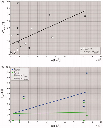
Furthermore, we presented the ratios between the mild-hyperthermic and thermally ablative effects, and IRE-TR, R_3ΔT13 and R_ΔT13, as a function of S_E-IRE(th) in Figure 9. Again, here we included ΔT_max, and u of the experimentally applied pulse parameters. Despite the small number of data points, this figure shows that an increase in the IRE-TR results in a constant mild-hyperthermic effects with MEDIAN(R_3ΔT13) = 31.75% and the range 0 ≤ R_3ΔT13 [%] ≤ 88.67. In addition, it also results in the increase of the thermally ablative effects with MEDIAN(R_ΔT13) = 4.57% with the range of 0 ≤ R_ΔT13 [%] ≤ 41.3.

Figure 9. Linear regression plots of R_3ΔT13 and R_ΔT13 data points as function of S_E-IRE(th). For a proper clarification of the data points, an extended version can be found in Supplementary Appendix 4 Figure A4.2. The ΔT_max and the u ranges were 1.9 ≤ ΔT_max [°C] ≤ 39, and 0.29×10⁷ ≤ u [J⋅m⁻³] ≤ 8.44 × 10⁷. Please note that the scale of the color bar of the energy density in this figure is different than the scales in Figure 8. In addition, the symbols at (4.83 × 10⁻⁵ m², 0.32%) and (4.83 × 10⁻⁵ m², 9.19%) have a gray background since the ΔT_max was not reported.

3.3.4. Thermal effects as function of energy density

The data obtained from Figures 8(C) and 9 were used in Figure 10 to show the relationships between u and ΔT_max, and u, R_3ΔT13 and R_ΔT13. These figures indicate that an increase in the u results in an increase of ΔT_max and R_3ΔT13, while R_ΔT13 remains almost constant.

Figure 10. (A) Linear regression plot of ΔT_max data points as function of the energy density. (B) Linear regression plots of R_3ΔT13 and R_ΔT13 data points as function of the energy density. Please note the change in X-axis in (B) in comparison to (A).

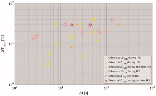
3.3.5. Estimation of time durations of thermal effects

Figure 11 illustrates the estimated time durations of both mild-hyperthermic and thermally ablative temperatures during IRE at the spatial point with the maximally simulated temperature increase ΔT_max. This was done for the studies included in meta-analysis with experimentally applied pulses. Please note that Δt_MH and Δt_TA were not calculated if they were provided by the included studies. Also, the data of Δt_MH and Δt_TA after the IRE treatment were included in Figure 11 only if they were provided by the included studies. To repeat, Δt_MH and Δt_TA represent the time durations of 3 ≤ ΔT_max [°C] < 13 (mild hyperthermia) and ΔT_max [°C] ≥ 13 (thermal ablation). The condition ‘ΔT_max [°C] ≥ 13’ at the spatial location with maximal simulated temperature increase (see Figure 5) indicates the presence of mild hyperthermia for a duration of Δt_MH prior to thermal ablation. Therefore, if the data from the included studies met the condition “ΔT_max [°C] ≥ 13”, then both values of Δt_MH and Δt_TA are plotted. Figure 11 shows that during the IRE treatment, the time duration for mild hyperthermia was MEDIAN(Δt_MH) = 15 s with 0 ≤ Δt_MH [s] ≤ 100, while the time duration for thermal ablation was MEDIAN(Δt_TA) = 0 s with 0 ≤ Δt_TA [s] ≤ 133.3. The median values include both calculated and extracted values. Furthermore, the studies from which Δt_MH and Δt_TA were extracted during and after IRE had medians of MEDIAN(Δt_MH) = 0 s with 0 ≤ Δt_MH [s] ≤ 180.7 and MEDIAN(Δt_TA) = 0 s 0 ≤ Δt_TA [s] ≤ 44.9.

Figure 11. The estimated time durations for both mild hyperthermia and thermal ablation as function ΔT_max. The term ‘Extracted’ means that Δt_MH and Δt_TA values were directly provided by the included studies, while the term ‘Calculated’ signifies that Δt_MH and Δt_TA were calculated using the assumptions stated in the Subsection 3.2.2.3. Estimation of time durations of mild-hyperthermic and thermally ablative temperatures. Please note that Δt represents the duration of mild-hyperthermic effect (3 °C ≤ ΔT_max < 13 °C) and thermal ablative effect (ΔT_max ≥ 13 °C) of an included study. The ΔT_max only represents the maximal temperature increase obtained from the included study. Also, note that the value of Δt_MH was 0 s for ΔT_max < 3 °C and the value of Δt_TA was 0 s for ΔT_max < 13 °C.

4. Discussion

4.1. Research questions

According to the predictions of the numerical models, the relative sizes of both locally mild-hyperthermic and thermally ablative effects in the IRE-TR, with respect to the IRE-TR, have approximate medians of 30 and 5%, respectively. Accordingly, IRE produces sufficient heat to thermally ablate small parts of the IRE-TR, and to raise the temperature within the range of 40 ≤ T [°C] < 50 in a third of the IRE-TR. This temperature range probably reduces the E_IRE(th) of the tissues and, consequently, enhances the IPE as was shown ex vivo for 43 °C in [20]. Mouse ectopic pancreatic cancer treated using an integrated IRE system with controllable laser heating at 42 °C was compared with standard IRE without additional heating. A complete tumor regression was observed in more than 50% of the tumor-bearing mice, while in the standard IRE group no complete regression was observed [19]. Results of this review predict that the IPE including the mild-hyperthermic effect dominates the IRE-TR with an approximate median of 95% (30% by combined contributions of mild-hyperthermic and IPE effects, and 65% by IPE effect only), implying that the IRE is based on the IPE with sufficient heat as adjuvant to enhance this effect. Again, it is important to notice that: first, the E_IRE(th) values in this review corresponds to the E_IRE(th) from the study from which S_E-IRE(th),Σ was extracted, and second, the pulse parameters on which the values of ΔT_max, S_3ΔT13,Σ and S_ΔT13,Σ depend, are different for each study.

The calculations of these medians were based on treated regions simulated by various types of setups. Specifically, the choice of the modeling parameters such as electrode type, electrical and thermal properties, and the type of BC can result in a different outcome of R_3ΔT13 and R_ΔT13. Nevertheless, most of the studies used for the calculation of these medians attempt to mimic the real world by utilizing dynamic electrical conductivity and perfusion. In addition, a Neumann boundary condition was mostly used for the electrical and thermal outer boundary conditions to estimate the upper limit of the induced temperatures. Therefore, these medians are likely to represent the thermal effects on the safe side.

The maximum temperature increase in Figure 8(A) shows that the pulses produce MEDIAN(ΔT_max) = 9.25 °C with 0.27 ≤ ΔT_max [°C] ≤ 135, but the exact predicted maximum temperature depends on the pulse parameters and other factors assumed in the model. One would expect that an increase in the pulse voltage and the total pulsing time would result in an increase of ΔT_max. However, these figures do not show a clear correlation between pulse voltage, pulsing time and temperature increase, since the temperature increase also depends on the pulse frequency (higher pulse frequency results in larger temperature increase) and on the model configuration. An adjustment of these properties results in different ΔT_max. For instance, ΔT_max, including the ratios of the mild-hyperthermic and thermally ablative regions with respect to IRE-TR, increases as a result of the increase of the pulse voltage, the pulse duration, the pulse frequency, the electrical and the thermal conductivity of the tissue and the number of electrode pairs, and by assuming Neumann boundary conditions at the electrode-medium interface and the outer surface of the model. Besides this, other factors yielding a higher predicted maximum temperature are a decrease in the distance between the electrodes, a decrease in the specific heat capacity and density, and exclusion of the blood perfusion term. Example of variation in both electrical and thermal properties is shown in Figure 7(A–E). These figures show differences between the values, even within the same tissue category.

The majority of the studies in Figure 8(A) did not actually apply the simulated pulses in experiments. In fact, some authors performed primarily a parametric study in which pulse, setup or tissue characteristics were varied, resulting in occasionally very large ΔT_max values [34,39,44,55]. Therefore, in Figure 8(B,C) we only included ΔT_max of the experimentally applied pulses with MEDIAN(ΔT_max) = 9.49 °C and the range 1 ≤ ΔT_max [°C] ≤ 39 for a median duration of 80 s (1.33 min) with (0.2 ≤ Total treatment time [min] ≤ 9), implying the presence of both mild-hyperthermic, and thermally ablative effects in the IRE-TR, which accords the findings in [13–15]. Please note that the duration of these effects depends on the selected experiment. For example, according to Figure 11 the duration of mild hyperthermia during IRE has a median of 15 s with the range 0 ≤ Δt [s] ≤ 100, while the duration of thermal ablation has a median of 0 s with the range 0 ≤ Δt [s] ≤ 133.3. These durations were calculated at a single point where ΔT_max was obtained (only during the temperature increase). Accordingly, the durations of both effects can be longer when considering the decay of the temperature post-IRE treatment.

Nevertheless, ΔT_max does not specify the size of these effects. Accordingly, in Figure 9 we plotted the ratios of the mild-hyperthermic and thermally ablative effects with respect to IRE-TR as a function of the IRE-TR. As expected, the increase of the IRE-TR results in the increase of the ΔT_max, which implies that the increase of IRE-TR raises the ΔT_max, and therefore, enlarges thermally ablative effect.

4.2. Energy density

Concerning the energy density of the experimentally applied pulses in Figure 10(A) and considering Equation 23(23) $$\mathrm{u}={\mathrm{\sigma }}_{\mathrm{init}}{\left|\frac{{\mathrm{V}}_{\mathrm{P}}}{\mathrm{D}}\right|}^2{\mathrm{t}}_{\mathrm{P}}{\mathrm{N}}_{\mathrm{P}}$$(23) one would expect to find a positive linear relationship between the energy density and ΔT_max. Indeed, by using the linear regression analysis we do observe that an increase in the energy density results in an increase in ΔT_max. However, the data points do not show a clear correlation, because of the many different system configurations used as mentioned above. This also applies to Figure 10(B), which shows the relationship between energy density and the ratios R_3ΔT13 and R_ΔT13.

4.3. Selection of model parameters

According to Figure 7(A–E), the selection of tissue properties varies between studies, even within the same tissue category. One reason for these variations is the inclusion of subcategories within the main categories. For example, ‘Brain’ can represent gray and white matter, ‘Blood vessel’ represents artery, blood and blood vessel, and ‘Muscle’ can represent longitudinal and transversal muscles in breast, prostate, and small intestine. Other reasons that can explain the variations are: (1) the anisotropicity and the heterogeneity of a tissue sample, (2) the location of the selected sample in an organ, (3) the animal species, and (4) the applied method to determine a property of a tissue type.

Due to the similarities of the values of the thermal properties in Figure 7(B–D), one would expect the perfusion term w_b to have a great influence on ΔT_max. Nevertheless, no correlation was found between these two parameters due to variation in the selection of other model properties, such as the boundary conditions and electrode type.

Finally, Figure 7(F) shows variation in the selection or calculation of E_IRE(th) between studies, even within the same tissue categories. Reasons that explain these variations are: (1) the application of different pulse parameters, (2) the choice of static or dynamic electrical conductivity, (3) the choice between the modeling of homogeneous or heterogeneous tissue type, (4) the applied electrode configuration; in comparison to plate electrodes, we expect larger mild-hyperthermic region in case of needle electrodes due to higher electric field density, with as a result a larger treated region and lower E_IRE(th).

Studies including the perfusion term in the bioheat transfer models applied constant blood perfusion. However, the blood perfusion is dynamic and depends on the magnitude and the duration of the thermal exposure, the tissue type, the size of the cancerous tissue, and whether a small or large animal model, or human model was used, as was shown in a review paper performed by Rossmann and Haemmerich [94] that summarized on the temperature and tissue-dependent thermal properties, including the blood perfusion, of several biological tissues at mild-hyperthermic and ablative temperatures. Based on figure 6 of [94], and since the medians of both simulation time and temperature increase of the included studies approximated 1.3 min (80 s) and 10 °C (47 °C relative to the assumed body temperature), we believe that temperature-dependent perfusion should be considered at T ≥ 43 °C for short total treatment time and at T ≥ 41 °C for long total treatment time. The latter would be preferred in treatment planning due to the presence of several needle pairs (more than 3 needle pairs in general; each pair with an approximation of 90 pulses and 10 test pulses) that may allow the extension of the total treatment time for more than 10 min. Nevertheless, the data about IRE-targeted organs are still limited. Therefore, further research should be performed to determine the influence of the magnitude and duration of thermal exposure.

4.4. Estimation of time durations of thermal effects

According to the extracted data and our simplified analysis, the mild-hyperthermic effect has a median time duration of 15 s, while thermally ablative effect has a median time duration of 0 s (ranges from 0 to ∼130 s) during the IRE treatment at the point with maximal temperature increase. Assuming a total treatment time of 80 s, this means that the combined medians of the time duration of the thermal effects would occur for approximately 20% of the treatment time (mild-hyperthermic effect for ∼20% and thermally ablative effect for 0%). However, these estimations relate to the duration during the IRE treatment itself and both effects will also last post IRE treatment. As a result, larger medians could be estimated for the total time durations. It is important to notice that the durations were calculated at the spatial point with ΔT_max. Since mild-hyperthermic temperatures spatially dominates the TA temperatures, the overall time duration of the mild-hyperthermic temperature, especially around the zones with T ≥ 50 °C (e.g. zones neighboring the electrodes), is longer than the time duration of TA effects. Furthermore, the studies included in the analysis used two electrodes in general. In the clinic, the number of electrode pairs is generally higher and could increase above 6 (more than 4 electrodes could be used), possibly resulting in further increase of ΔT_max and the mild-hyperthermic and ablative time durations. In particular, this applies for mild-hyperthermic effect, since an adequate order of the electrode pairs could avoid the extension of TA effects as was shown by O’Brien et al. [95]. O’Brien et al. showed in an ex vivo study using a perfused porcine liver model that cycled pulsing schemes increase the treatment zone size and maintain a low tissue temperature compared to conventional pulsing schemes.

Our analysis can include estimation errors, since (1) the temperature profile has a temporal exponential profile if our simplified assumptions were not taken into consideration, and (2) only some of the simplified assumptions were assumed by the included studies. However, by comparing the extracted time durations with the calculated ones, a deviation of ≤22% was found. Finally, one must note that the included studies in which multiple electrode pairs were used did not consider the delays between the pulse sequences. In the clinic, delays are applied between the pulse sequences of different electrode pairs, both to recharge the pulse generator and to reduce the produced ΔT_max. By taking these delays into consideration, one would expect a reduction in thermal effects. Nevertheless, only a slight reduction of the combined median time duration of the thermal effects is expected since only two out of the 12 included studies applied IRE with 4 electrodes which involve activating four different electrode pairs during IRE [33,41].

4.5. Inclusion of vascular structures

The majority of the included studies did not incorporate vascular structures with blood vessels in the models [3,24,26, 39–42]. Due to the high electrical conductivity of blood, the inclusion of vascular structures in or in close proximity of the treatment volume can result in distortion of the distribution of the electric field strength inside the treatment volume. Consequently, neighboring areas with relatively high or low electric field strength can emerge, resulting in undesirable overtreatment or undertreatment of those areas with possible clinical complications or treatment failure as a consequence. Several experimental and in silico studies showed that the distortion of the distribution of the electric field strength resulted in reduction of the electric field strength in areas inside the treated zone adjacent to the vascular structure; the ‘electric field sink’ effect [54,62,71,96]. For example, Goldberg et al. experimentally showed undertreated zones adjacent to vascular structures in the liver of rats after application of IRE between two electrode plates [54]. We therefore recommend the inclusion of vascular structures in treatment planning to avoid possible undesired poor quality treatments and to accurately predict the local electric field and temperature distribution.

Furthermore, large blood vessels can yield a substantial cooling effect in the ablated region, similar as for RFA and MWA thermal ablation, which can result in a local temperature decrease of more than 20 °C [97]. Several experimental and in silico studies showed a much lower temperature increase in the vicinity of a large blood vessel during RFA or MWA, dependent on the orientation of the vessel and its distance to the applicator [97–100]. This demonstrates the relevance of accounting for large blood vessels also in IRE models, since a local cooling effect may significantly affect the produced thermal increase in the close vicinity of large vessels, which may result locally in only an irreversible permeabilization effect. Van Gemert et al. demonstrated in a 1D analytical IRE model that a large blood vessel at ∼5 mm distance from a needle can produce a local cooling effect up to a few degrees [64]. A simplified model not including large vessels would be sufficient when for example evaluating maximum temperature levels achievable during IRE. However, when accurate predictions of the local temperature distribution are required, the effect of nearby large blood vessels should be accounted for in the models.

4.6. Challenges of simulations

The results presented in this review are based on calculations extracted from several studies with various simulated setups. Specifically, the extracted data may include errors, due to e.g. inaccurate modeling of the media (homogeneous instead of heterogeneous), inaccurate modeling of the simulated setup, inaccurate choice of boundary conditions, inaccurate assignment/modeling of electrical and thermal properties, and inaccurate choice of pulse characteristics (e.g. not modeling the delays within a single pulse sequence and between separate pulse sequences of different electrode pairs will result in overestimations of temperature). Another example is the modeling of σ(T), in which σ was modeled as a function of temperature (see Supplementary Appendix 4 for more details). Specifically, the electrical conductivity can increase by 1–3% per 1 °C [50]. However, the increase of σ stops after a certain temperature due to the vaporization process of water in the medium. Therefore, a certain threshold should be included in σ(T) and σ(E, T) to avoid σ to further increase after a certain temperature. This temperature is typically 100 °C, which was applied by several RFA studies [101,102]. Despite these uncertainties in the modeling studies, the data obtained in this review still provides useful insight in the possible thermal elevation by IRE.

4.7. Take-home message

This review demonstrates the likelihood of direct thermal ablation in comparatively small regions and mild-hyperthermic effects in a large part of the IRE-TR, predicting the significant presence of hyperthermia in IRE. Even though the thermally ablated regions were relatively small, care must be taken for large temperature increases, especially in case of adjacent critical structures. This review focused on studies that performed numerical calculations, which are very useful to obtain insight in the general impact of various pulse parameters on the effect of IRE. Numerical calculations typically do not model nanopore effects and assume a simplified anatomy, not accounting for variations in tissue properties. Nevertheless, results clearly indicate that IRE can have significant thermal effects. Therefore, further in vivo research should investigate thermal effects of IRE to determine the relative size of the irreversible permeabilized region in which mild-hyperthermic and thermally ablative temperatures are achieved and significantly contribute to tumor ablation. These insights will help to optimize clinical protocols of IRE.

The expression ‘non-thermal IRE’ is generally used, (1) because IRE is a technique based on the creation of nanopores in the cell membrane, and (2) to distinguish IRE from thermal ablation techniques such as RFA and MWA. However, due to the significant presence of thermal effects (including 40 ≤ T [°C] < 50), and since literature data demonstrate that thermal effects clearly do contribute to the tumor ablation, one might consider avoiding the expression ‘non-thermal’ and start focusing on researching the mild-hyperthermic contribution to further optimize IRE-treatment.

Disclosure statement

The author(s) declared the following potential conflicts of interest with respect to the research, authorship, and/or publication of this article: K. P. van Lienden, T. M. van Gulik and M.R. Meijerink are paid consultants for Angio-Dynamics. Angio-Dynamics had no role in the design of the study; in the collection, analyses, or interpretation of data; in the writing of the manuscript, or in the decision to publish the results.

Additional information

Funding

This research was financially supported by the Dutch Cancer Society [grant UvA 2014-7244].

References

- Rubinsky B, Onik G, Mikus P. Irreversible electroporation: a new ablation modality – clinical implications. Technol Cancer Res Treat. 2007;6(1):37–48.
- Maor E, Ivorra A, Rubinsky B. Non thermal irreversible electroporation: novel technology for vascular smooth muscle cells ablation. PloS One. 2009;4(3):e4757.
- Davalos RV, Mir LM, Rubinsky B. Tissue ablation with irreversible electroporation. Ann Biomed Eng. 2005;33(2):223–231.
- Mercadal B, Beitel-White N, Aycock KN, et al. Dynamics of cell death after conventional IRE and H-FIRE treatments. Ann Biomed Eng. 2020;8:1451–1462.
- Pillai K, et al. Heat sink effect on tumor ablation characteristics as observed in monopolar radiofrequency, bipolar radiofrequency, and microwave, using ex vivo calf liver model. Medicine. 2015;94(9):e580.
- Vogel JA, van Veldhuisen E, Agnass P, et al. Time-dependent impact of irreversible electroporation on pancreas, liver, blood vessels and nerves: a systematic review of experimental studies. PloS One. 2016;11(11):e0166987.
- Scheltema MJV, van den Bos W, de Bruin DM, et al. Focal vs extended ablation in localized prostate cancer with irreversible electroporation; a multi-center randomized controlled trial. BMC Cancer. 2016;16(1):299.
- Buijs M, van Lienden KP, Wagstaff PG, et al. Irreversible electroporation for the ablation of renal cell carcinoma: a prospective, human, in vivo study protocol (IDEAL Phase 2b). JMIR Res Protoc. 2017;6(2):e21.
- Martin RCG, Kwon D, Chalikonda S, et al. Treatment of 200 locally advanced (stage III) pancreatic adenocarcinoma patients with irreversible electroporation safety and efficacy. Ann Surg. 2015;262(3):486–494.
- Coelen RJS, Vogel JA, Vroomen LGPH, et al. Ablation with irreversible electroporation in patients with advanced perihilar cholangiocarcinoma (ALPACA): a multicentre phase I/II feasibility study protocol. BMJ Open. 2017;7(9):e015810.
- Narayanan G, Hosein PJ, Beulaygue IC, et al. Percutaneous image-guided irreversible electroporation for the treatment of unresectable, locally advanced pancreatic adenocarcinoma. J Vasc Interv Radiol. 2017;28(3):342–348.
- Vogel JA, Rombouts SJ, de Rooij T, et al. Induction chemotherapy followed by resection or irreversible electroporation in locally advanced pancreatic cancer (IMPALA): a prospective cohort study. Ann Surg Oncol. 2017;24(9):2734–2743.
- van den Bos W, Scheffer HJ, Vogel JA, et al. Thermal energy during irreversible electroporation and the influence of different ablation parameters. J Vasc Interv Radiol. 2016;27(3):433–443.
- Faroja M, Ahmed M, Appelbaum L, et al. Irreversible electroporation ablation: is all the damage nonthermal? Radiology. 2013;266(2):462–470.
- Wagstaff PGK, et al. Irreversible electroporation of the porcine kidney: temperature development and distribution. Urol Oncol Semin Orig Investig. 2015;33(4):168.e1–7.
- Agnass P, et al. Thermodynamic profiling during irreversible electroporation in porcine liver and pancreas: a case study series. J Clin Transl Res. 2020;5(3).
- Bakker A, van der Zee J, van Tienhoven G, et al. Temperature and thermal dose during radiotherapy and hyperthermia for recurrent breast cancer are related to clinical outcome and thermal toxicity: a systematic review. Int J Hyperthermia. 2019;36(1):1024–1039.
- Moritz AR, Henriques FC. Studies of thermal injury: II. The relative importance of time and surface temperature in the causation of cutaneous burns. Am J Pathol. 1947;23(5):695–720.
- Sapareto SA, Dewey WC. Thermal dose determination in cancer-therapy. Int J Radiat Oncol Biol Phys. 1984;10(6):787–800.
- Edelblute CM, Hornef J, Burcus NI, et al. Controllable moderate heating enhances the therapeutic efficacy of irreversible electroporation for pancreatic cancer. Sci Rep. 2017;7(1):11767.
- Hutton B, Salanti G, Caldwell DM, et al. The PRISMA extension statement for reporting of systematic reviews incorporating network meta-analyses of health care interventions: checklist and explanations. Ann Intern Med. 2015;162(11):777–784.
- Moher A, Liberati J, Tetzlaff DG. Altman D, The PRISMA Group. Preferred reporting items for systematic reviews and meta-analyses: the PRISMA statement. PLoS Med. 2009;6(7):e1000097.
- Dewhirst MW, Viglianti BL, Lora-Michiels M, et al. Basic principles of thermal dosimetry and thermal thresholds for tissue damage from hyperthermia. Int J Hyperthermia. 2003;19(3):267–294.
- Edd JF, Horowitz L, Davalos RV, et al. In vivo results of a new focal tissue ablation technique: irreversible electroporation. IEEE Trans Biomed Eng. 2006;53(7):1409–1415.
- Al-Sakere B, André F, Bernat C, et al. Tumor ablation with irreversible electroporation. PloS One. 2007;2(11):e1135.
- Edd JF, Davalos RV. Mathematical modeling of irreversible electroporation for treatment planning. Technol Cancer Res Treat. 2007;6(4):275–286.
- Davalos RV, Rubinsky B. Temperature considerations during irreversible electroporation. Int J Heat Mass Transf. 2008;51(23-24):5617–5622.
- Daniels C, Rubinsky B. Electrical field and temperature model of nonthermal irreversible electroporation in heterogeneous tissues. J Biomech Eng Trans ASME. 2009;131(7):071006.
- Neal RE, Davalos RV. The feasibility of irreversible electroporation for the treatment of breast cancer and other heterogeneous systems. Ann Biomed Eng. 2009;37(12):2615–2625.
- Shafiee H, Garcia PA, Davalos RV. A preliminary study to delineate irreversible electroporation from thermal damage using the Arrhenius equation. J Biomech Eng Trans ASME. 2009;131(7):074509.
- Garcia PA, Rossmeisl JH, Neal RE, et al. Intracranial nonthermal irreversible electroporation: in vivo analysis. J Membrane Biol. 2010;236(1):127–136.
- Golberg A, Rubinsky B. A statistical model for multidimensional irreversible electroporation cell death in tissue. BioMed Eng Online. 2010;9(1):13.
- Maor E, Ivorra A, Mitchell JJ, et al. Vascular smooth muscle cells ablation with endovascular nonthermal irreversible electroporation. J Vasc Interv Radiol. 2010;21(11):1708–1715.
- Maor E, Rubinsky B. Endovascular nonthermal irreversible electroporation: a finite element analysis. J Biomech Eng Trans ASME. 2010;132(3):031008.
- Neal RE, Singh R, Hatcher HC, et al. Treatment of breast cancer through the application of irreversible electroporation using a novel minimally invasive single needle electrode. Breast Cancer Res Treat. 2010;123(1):295–301.
- Phillips M, Maor E, Rubinsky B. Nonthermal irreversible electroporation for tissue decellularization. J Biomech Eng Trans ASME. 2010;132(9):091003.
- Sano MB, Neal RE, Garcia PA, et al. Towards the creation of decellularized organ constructs using irreversible electroporation and active mechanical perfusion. BioMed Eng Online. 2010;9(1):83.
- Zhang Y, Guo Y, Ragin AB, et al. MR imaging to assess immediate response to irreversible electroporation for targeted ablation of liver tissues: preclinical feasibility studies in a rodent model. Radiology. 2010;256(2):424–432.
- Adeyanju OO, Al-Angari HM, Sahakian AV. The improvement of irreversible electroporation therapy using saline-irrigated electrodes: a theoretical study. Technol Cancer Res Treat. 2011;10(4):347–360.
- Garcia PA, Rossmeisl JH, Neal RE, et al. A parametric study delineating irreversible electroporation from thermal damage based on a minimally invasive intracranial procedure. BioMed Eng Online. 2011;10(1):34.
- Phillips M, Maor E, Rubinsky B. Principles of tissue engineering with nonthermal irreversible electroporation. J Heat Transf Trans ASME. 2011;133(1):011004.
- Županič A, Miklavčič D. Tissue heating during tumor ablation with irreversible electroporation. Electrotechnical Rev. 2011;78(1-2):42–47.
- Arena CB, Szot CS, Garcia PA, et al. A three-dimensional in vitro tumor platform for modeling therapeutic irreversible electroporation. Biophys J. 2012;103(9):2033–2042.
- Mandel Y, Rubinsky B. Treatment of uveal melanoma by nonthermal irreversible electroporation: electrical and bioheat finite element model of the human eye. J Heat Transf Trans ASME. 2012;134(11):111101.
- Neal RE, Garcia PA, Robertson JL, et al. Experimental characterization and numerical modeling of tissue electrical conductivity during pulsed electric fields for irreversible electroporation treatment planning. IEEE Trans Biomed Eng. 2012;59(4):1076–1085.
- Sahakian AV, Al-Angari HM, Adeyanju OO. Electrode activation sequencing employing conductivity changes in irreversible electroporation tissue ablation. IEEE Trans Biomed Eng. 2012;59(3):604–607.
- Kurata K, Ueno R, Matsushita M, et al. Experimental and analytical studies on contact irreversible electroporation for superficial tumor treatment. JBSE. 2013;8(4):306–318.
- Mandel Y, Malki G, Adawi E, et al. Hemorrhage control of liver injury by short electrical pulses. PloS One. 2013;8(8):e49852.
- Neal RE, Smith RL, Kavnoudias H, et al. The effects of metallic implants on electroporation therapies: feasibility of irreversible electroporation for brachytherapy salvage. Cardiovasc Intervent Radiol. 2013;36(6):1638–1645.
- Qin ZP, Jiang J, Long G, et al. Irreversible electroporation: an in vivo study with dorsal skin fold chamber. Ann Biomed Eng. 2013;41(3):619–629.
- Srimathveeravalli G, Wimmer T, Monette S, et al. Evaluation of an endorectal electrode for performing focused irreversible electroporation ablations in the swine rectum. J Vasc Interv Radiol. 2013;24(8):1249–1256.
- Wimmer T, Srimathveeravalli G, Gutta N, et al. Comparison of simulation-based treatment planning with imaging and pathology outcomes for percutaneous CT-guided irreversible electroporation of the porcine pancreas: a pilot study. J Vasc Interv Radiol. 2013;24(11):1709–1718.
- Garcia PA, Davalos RV, Miklavcic D. A numerical investigation of the electric and thermal cell kill distributions in electroporation-based therapies in tissue. PloS One. 2014;9(8):e103083.
- Golberg A, Bruinsma BG, Uygun BE, et al. Tissue heterogeneity in structure and conductivity contribute to cell survival during irreversible electroporation ablation by electric field sinks. Sci Rep. 2015;5(1):8485.
- Kurata K, Nomura S, Takamatsu H. Three-dimensional analysis of irreversible electroporation: estimation of thermal and non-thermal damage. Int J Heat Mass Transf. 2014;72:66–74.
- Neal RE, Millar JL, Kavnoudias H, et al. In vivo characterization and numerical simulation of prostate properties for non-thermal irreversible electroporation ablation. Prostate. 2014;74(5):458–468.
- Neal RE, Rossmeisl JH, D’Alfonso V, et al. In vitro and numerical support for combinatorial irreversible electroporation and electrochemotherapy glioma treatment. Ann Biomed Eng. 2014;42(3):475–487.
- Nickfarjam A, Firoozabadi SMP. Parametric study of irreversible electroporation with different needle electrodes: electrical and thermal analysis. Int J Hyperthermia. 2014;30(5):335–347.
- Phillips, M. The effect of small intestine heterogeneity on irreversible electroporation treatment planning. J Biomech Eng Trans ASME. 2014;136(9):091009.
- Dermol J, Miklavcic D. Mathematical models describing Chinese hamster ovary cell death due to electroporation in vitro. J Membrane Biol. 2015;248(5):865–881.
- Ivey JW, Latouche EL, Sano MB, et al. Targeted cellular ablation based on the morphology of malignant cells. Sci Rep. 2015;5(1):17157.
- Kos B, Voigt P, Miklavcic D, et al. Careful treatment planning enables safe ablation of liver tumors adjacent to major blood vessels by percutaneous irreversible electroporation (IRE). Radiol Oncol. 2015;49(3):234–241.
- Neal RE, Garcia PA, Kavnoudias H, et al. In vivo irreversible electroporation kidney ablation: experimentally correlated numerical models. IEEE Trans Biomed Eng. 2015;62(2):561–569.
- van Gemert MJC, Wagstaff PGK, de Bruin DM, et al. Irreversible electroporation: just another form of thermal therapy? Prostate. 2015;75(3):332–335.
- Wimmer T, Srimathveeravalli G, Gutta N, et al. Planning irreversible electroporation in the porcine kidney: are numerical simulations reliable for predicting empiric ablation outcomes? Cardiovasc Intervent Radiol. 2015;38(1):182–190.
- Sharabi S, Kos B, Last D, et al. A statistical model describing combined irreversible electroporation and electroporation-induced blood-brain barrier disruption. Radiol Oncol. 2016;50(1):28–38.
- Srimathveeravalli G, Cornelis F, Mashni J, et al. Comparison of ablation defect on MR imaging with computer simulation estimated treatment zone following irreversible electroporation of patient prostate. SpringerPlus. 2016;5(1):219.
- Campelo S, et al. An evaluation of irreversible electroporation thresholds in human prostate cancer and potential correlations to physiological measurements. APL Bioeng. 2017;1(1):016101.
- Garcia PA, Kos B, Rossmeisl JH, et al. Predictive therapeutic planning for irreversible electroporation treatment of spontaneous malignant glioma. Med Phys. 2017;44(9):4968–4980.
- Latouche EL, Sano MB, Lorenzo MF, et al. Irreversible electroporation for the ablation of pancreatic malignancies: a patient-specific methodology. J Surg Oncol. 2017;115(6):711–717.
- Qasrawi R, Silve L, Burdio F, et al. Anatomically realistic simulations of liver ablation by irreversible electroporation: impact of blood vessels on ablation volumes and undertreatment. Technol Cancer Res Treat. 2017;16(6):783–792.
- Sung CK, Kim HB, Jung JH, et al. Histological and mathematical analysis of the irreversibly electroporated liver tissue. Technol Cancer Res Treat. 2017;16(4):488–496.
- Wasson EM, Ivey JW, Verbridge SS, et al. The feasibility of enhancing susceptibility of glioblastoma cells to IRE using a calcium adjuvant. Ann Biomed Eng. 2017;45(11):2535–2547.
- Yao CG, Dong SL, Zhao YJ, et al. Bipolar microsecond pulses and insulated needle electrodes for reducing muscle contractions during irreversible electroporation. IEEE Trans Biomed Eng. 2017;64(12):2924–2937.
- Yoshimatsu S, Yoshida M, Kurata K, et al. Development of contact irreversible electroporation using a comb-shaped miniature electrode. J Therm Sci Technol. 2017;12(2):JTST0023–JTST0023.
- Castellvi Q, Mercadal B, Moll X, et al. Avoiding neuromuscular stimulation in liver irreversible electroporation using radiofrequency electric fields. Phys Med Biol. 2018;63(3):035027.
- Ritter A, Bruners P, Isfort P, et al. Electroporation of the liver: more than 2 concurrently active, curved electrodes allow new concepts for irreversible electroporation and electrochemotherapy. Technol Cancer Res Treat. 2018;17:153303381880999.
- Yang YJ, Moser MAJ, Zhang E, et al. Development of a statistical model for cervical cancer cell death with irreversible electroporation in vitro. PloS One. 2018;13(4):e0195561.
- Gallinato O, Denis de Senneville B, Seror O, et al. Numerical workflow of irreversible electroporation for deep-seated tumor. Phys Med Biol. 2019;64(5):055016.
- O’Brien TJ, Bonakdar M, Bhonsle S, et al. Effects of internal electrode cooling on irreversible electroporation using a perfused organ model. Int J Hyperthermia. 2018;35(1):44–55.
- Gallinato OPC. 2019. IRENA: a finite volume method based software for the numerical assessment of clinical IRE (version 1.0) APP IDDN.FR.001.080021.000.S.P.2019.000.31230 [Online]. Available from: https://team.inria.fr/monc/software/.
- Henriques FC, Moritz AR. Studies of thermal injury: I. The conduction of heat to and through skin and the temperatures attained therein. A theoretical and an experimental investigation. Am J Pathol. 1947;23(4):530–549.
- Moritz AR. Studies of thermal injury: III. The pathology and pathogenesis of cutaneous burns. An experimental study. Am J Pathol. 1947;23(6):915–941.
- Henriques FC Jr. Studies of thermal injury: V. The predictability and the significance of thermally induced rate processes leading to irreversible epidermal injury. Arch Pathol. 1947;43(5):489–502.
- Yarmolenko PS, Moon EJ, Landon C, et al. Thresholds for thermal damage to normal tissues: an update. Int J Hyperthermia. 2011;27(4):320–343.
- van Rhoon GC, Samaras T, Yarmolenko PS, et al. CEM43A degrees C thermal dose thresholds: a potential guide for magnetic resonance radiofrequency exposure levels? Eur Radiol. 2013;23(8):2215–2227.
- Mouratidis PXE, Rivens I, Civale J, et al. Relationship between thermal dose and cell death for “rapid” ablative and “slow” hyperthermic heating. Int J Hyperthermia. 2019;36(1):229–243.
- Pearce J. Relationship between Arrhenius models of thermal damage and the CEM 43 thermal dose (SPIE BiOS). SPIE. 2009;7181:718104.
- Pearce JA. Comparative analysis of mathematical models of cell death and thermal damage processes. Int J Hyperthermia. 2013;29(4):262–280.
- Ivorra A, Rubinsky B. In vivo electrical impedance measurements during and after electroporation of rat liver. Bioelectrochemistry. 2007;70(2):287–295.
- Pavlin M, Kandušer M, Reberšek M, et al. Effect of cell electroporation on the conductivity of a cell suspension. Biophys J. 2005;88(6):4378–4390.
- Corovic S, Lackovic I, Sustaric P, et al. Modeling of electric field distribution in tissues during electroporation. BioMed Eng Online. 2013;12(1):16.
- Hasgall PA, et al. 2018. IT’IS Database for thermal and electromagnetic parameters of biological tissues. Available from: https://itis.swiss/virtual-population/tissue-properties/database/database-summary/.
- Rossmanna C, Haemmerich D. Review of temperature dependence of thermal properties, dielectric properties, and perfusion of biological tissues at hyperthermic and ablation temperatures. Crit Rev Biomed Eng. 2014;42(6):467–492.
- J. O’Brien T, et al. Cycled pulsing to mitigate thermal damage for multi-electrode irreversible electroporation therapy. Int J Hyperthermia. 2019;36(1):953–963.
- Marcan M, Kos B, Miklavcic D. Effect of blood vessel segmentation on the outcome of electroporation-based treatments of liver tumors. PloS One. 2015;10(5):e0125591.
- Ringe KI, Lutat C, Rieder C, et al. Experimental evaluation of the heat sink effect in hepatic microwave ablation. PloS One. 2015;10(7):e0134301.
- Zorbas G, Samaras T. A study of the sink effect by blood vessels in radiofrequency ablation. Comput Biol Med. 2015;57:182–186.
- Jiang K, Chen J, Liu Y, et al. Heat-irrigate effect’ of radiofrequency ablation on relevant regional hepatocyte in living swine liver-initial study on pathology. Cell Biochem Biophys. 2015;72(1):37–41.
- Chen RD, Lu F, Wu F, et al. An analytical solution for temperature distributions in hepatic radiofrequency ablation incorporating the heat-sink effect of large vessels. Phys Med Biol. 2018;63(23):235026.
- Gonzalez-Suarez A, Berjano E. Comparative analysis of different methods of modeling the thermal effect of circulating blood flow during RF cardiac ablation. IEEE Trans Biomed Eng. 2016;63(2):250–259.
- Trujillo M, Bon J, Berjano E. Computational modelling of internally cooled wet (ICW) electrodes for radiofrequency ablation: impact of rehydration, thermal convection and electrical conductivity. Int J Hyperthermia. 2017;33(6):624–634.