The impact of data selection and fitting on SAR estimation for magnetic nanoparticle heating

Abstract

Background

Magnetic fluid heating has great potential in the fields of thermal medicine and cryopreservation. However, variations among experimental parameters, analysis methods and experimental uncertainty make quantitative comparisons of results among laboratories difficult. Herein, we focus on the impact of calculating the specific absorption rate (SAR) using Time-Rise and Box-Lucas fitting. Time-Rise assumes adiabatic conditions, which is experimentally unachievable, but can be reasonably assumed (quasi-adiabatic) only for specific and limited evaluation times when heat loss is negligible compared to measured heating rate. Box-Lucas, on the other hand, accounts for heat losses but requires longer heating.

Methods

Through retrospective analysis of data obtained from two laboratories, we demonstrate measurement time is a critical parameter to consider when calculating SAR. Volumetric SAR were calculated using the two methods and compared across multiple iron-oxide nanoparticles.

Results

We observed the lowest volumetric SAR variation from both fitting methods between 1–10 W/mL, indicating an ideal SAR range for heating measurements. Furthermore, our analysis demonstrates that poorly chosen fitting method can generate reproducible but inaccurate SAR.

Conclusion

We provide recommendations to select measurement time for data analysis with either Modified Time-Rise or Box-Lucas method, and suggestions to enhance experimental precision and accuracy when conducting heating experiments.

Keywords:

• Magnetic iron oxide nanoparticles
• magnetic fluid hyperthermia
• data analysis
• nanowarming
• specific absorption rate calculation

Introduction

Magnetic nanoparticle or magnetic fluid hyperthermia (MFH) is a cancer treatment indicated as an adjunct treatment for recurrent glioblastoma with radiation therapy [1,2]. It comprises direct delivery of a magnetic fluid, i.e. aqueous suspension of iron oxide nanoparticles, into the tumor that generates heat when exposed to an alternating magnetic field [1,3–6]. The therapeutic agent is heat produced by the nanoparticles, and thus potency or heating capability of the suspension is a critical parameter for treatment planning and execution [7–9]. Additionally, emerging clinical applications, such as neuromodulation and cryopreservation of tissues, exploit controlled heat production with magnetic nanoparticles [10–12]. A direct comparison of iron oxide nanoparticle (IONP) heating capability for MFH across laboratories has proven unreliable, thus challenging quantitative comparisons among IONP formulations to determine clinical suitability, and inhibiting development of universal standardized methodologies for clinical translation [13,14].

Hysteresis loss power heat generated by magnetic nanoparticles is often measured with simple constant pressure (atmospheric) calorimetric methods, from which normalized heating power is estimated. The calorimeter often comprises a thermally insulated vessel with thermometer that is placed within the induction coil. A known volume of sample, or nanoparticle suspension having a known concentration, is placed into the vessel. Heat generated by the nanoparticles with AMF is absorbed by the suspending medium (e.g. water), causing a temperature change (ΔT) which is measured. It is typically assumed that the temperature of the sample is reasonably homogeneous, and that the temperature probe measurement accurately reflects the temperature throughout the sample volume. Using the sample specific heat (i.e. typically assumed to be the medium), estimates of the energy absorbed are then performed from analysis of changes of temperature within a specified time interval. An inherent assumption with this methodology is that the temperature changes measured in the sample occur only from heat generated by the nanoparticles in response to the AMF. Heat transfer between the sample and the environment, if unaccounted for, will inevitably generate erroneous values of loss power heating. The method of analysis, therefore must be carefully chosen to incorporate the limitations of the measurement methods and/or apparatus, and the data collected. It is often the case that estimation of heating power implicitly assumes adiabatic conditions (Equation (1)(1) $$\mathit{SLP}=\frac{P}{m_{Fe}}=\frac{m_s}{m_{Fe}}·c·\frac{dT}{dt}$$(1) ). This condition may not be strictly possible given that the induction coil can be either heat source or heat sink, depending on specific properties of its operation (e.g. current load, voltage, cooling capacity of coolant, etc.). Further, this method is limited by errors within temperature measurements, which arise from limitations of equipment resolution, experimental setup (heat exchange with surroundings, field inhomogeneities/instabilities, chemical/morphological changes in the sample over time), execution, uncertainty in iron mass determination and thermometry measurement [15–18]. Additionally, various methods are used to fit and analyze data, further contributing to reduced consistency and reliability [8,18,19]. Often method(s) used to estimate normalized dissipated power from temperature-time measurements is/are fixed without considering the underlying assumptions for the calculations, and limitations of the apparatus used to measure heat generated. For iron containing magnetic nanoparticles, specific loss power (SLP) is often reported as a function of iron mass to indicate IONP heating capability (W/g Fe) [3,14]. Assuming no heat exchange with surroundings, no work performed, no chemical or physical (change of state) changes in the sample, and constant pressure, the relationship between SLP, power (P) and the change in temperature are: (1) $$\mathit{SLP}=\frac{P}{m_{Fe}}=\frac{m_s}{m_{Fe}}·c·\frac{dT}{dt}$$(1) where c = the specific heat (J/g.^oC), m_s = sample mass, m_Fe = the mass of iron (g), and dT/dt is the temperature change within a defined time interval, or first derivative of the temperature as a function of time (^oC/s). Volumetric SAR can be described as power output normalized to sample volume (SAR_v, W/mL): (2) $${\mathit{SAR}}_v=\rho ·c·\frac{dT}{dt}=\mathit{SLP}\mathrm{·}{c}_{Fe}$$(2) where, ρ is the sample density, c_Fe is the iron concentration in the sample. While SAR_v and SLP can be easily converted as shown in Equation (2)(2) $${\mathit{SAR}}_v=\rho ·c·\frac{dT}{dt}=\mathit{SLP}\mathrm{·}{c}_{Fe}$$(2) , there are advantages to working with SAR_v alone from the point of view of calorimetry and heat transfer. First, the sample density and specific heat (i.e. water, tissue or other) are largely unchanged for low concentrations of nanoparticles and can be directly measured prior to calorimetry. This means that SAR_v can be reasonably estimated based on the dT/dt even without precise knowledge of iron content or SLP as long as our calorimetric assumptions hold. This means that estimation of error in fitting SAR_v, a main feature of the present work, is more directly correlated to the calorimetry itself and not compounded by possible errors from iron concentration estimation [20–23]. In addition to being a concept that can be directly related to the calorimetric measurement it also becomes an estimate of heat that can be produced by iron oxide nanoparticles in complex systems (i.e. tissues/organs) for known IONP concentrations [8,20,21,24]. This in turn can be used in computational heat transfer modeling efforts employing the bioheat transfer equation. We report results of comparisons between fitting methods and power output from heating measurements obtained for several samples in two different laboratories. For the evaluated datasets, sample density was consistent; however, IONP concentrations among samples varied. Therefore, we use SAR_v for comparison because it correlates with power for the scope of the evaluated datasets.

Using the Time-Rise method, SLP, and SAR_v are calculated from the slope (dT/dt) by fitting T vs t [18,19]. The Time-Rise calculation can be used during low heat loss conditions (i.e. a well-insulated system, short experimental evaluation times, and low SAR_v).

Box-Lucas analysis assumes a non-adiabatic system where the convective heat losses can be approximated as a loss term with the difference between the sample and ambient temperature. As shown in Equation (3)(3) $$T=\frac{P}{L}\left(1-e^{-t/\left(\frac{c}{L}\right)}\right)+T_0$$(3) , Wildeboer et al. provide a derivation of the Box-Lucas equation based on this assumption which results in an exponential growth dependence of temperature as a function of time [14] (Figure 1): (3) $$T=\frac{P}{L}\left(1-e^{-t/\left(\frac{c}{L}\right)}\right)+T_0$$(3) where, L is the heat loss from the sample, and P is the power generated by the sample. Multiplying the amplitude (P/L) and exponential factor (L/c) from fitting the Box-Lucas equation (Equation (4)) provides P/c is shown in Equations (1)(1) $$\mathit{SLP}=\frac{P}{m_{Fe}}=\frac{m_s}{m_{Fe}}·c·\frac{dT}{dt}$$(1) and (2)(2) $${\mathit{SAR}}_v=\rho ·c·\frac{dT}{dt}=\mathit{SLP}\mathrm{·}{c}_{Fe}$$(2) to be equivalent to dT/dt and can be used to calculate SLP, and SAR_v. We note that radiative heat losses can be linear and important when ΔT ≪ T.

Figure 1. Schematic of adiabatic, and non-adiabatic heating curves during the heating (coil on) and cooling (coil off) phases of a heat experiment. Common fitting time-frames to calculate SAR_v include: Time-Rise, Box-Lucas, Steady State, and Decay.

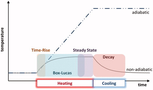
Several alternate calculation methods have been proposed to compensate for heat losses. Specifically, measurements of the temperature steady state occurring at the end of the heating phase of the experiment or the temperature decay during the cooling phase can be used to directly calculate the heating losses of the system (Figure 1) [14–16,25,26]. Calculation of heat losses allows for the determination if linear heat losses are dominant [14]. For convenience, SAR_v is often calculated from the heating phase of the experiment using either Time-Rise (i.e. initial slope), or Box-Lucas fitting. Due to the different assumptions, discrepancies between estimates of SAR_v obtained from Time-Rise and Box-Lucas fitting can occur [18,19,27]. The many sources of error within the measuring equipment and physical sample can affect the accuracy and precision of SAR_v [14,16,26–28]. The selection of Time-Rise or Box-Lucas fitting to calculate SAR_v will variably affect precision and accuracy depending on the selected measurement time interval and variance within the data. Herein, we perform a direct comparison between Box-Lucas and Time-Rise fitting methods by reanalyzing previously published datasets to determine the appropriate conditions (optimal SAR_v range, length of evaluation time and starting times) for using Box-Lucas and Time-Rise fitting methods.

Materials and methods

Datasets

These two datasets were collected from several different IONPs, under different conditions (frequency, magnetic field strength, IONP concentration), from two different laboratories (Johns Hopkins University & University of Minnesota). The acquisition time of the temperature-time datasets was sufficient to enable a comparison of variations in evaluation time.

Retrospective data analysis

Retrospective data analysis was performed with MATLAB 2012 b on temperature-time datasets published in Bordelon et al. and Etheridge et al. [19,25]. Four different evaluation time scenarios were compared: (1) 30 s; (2) 60 s; (3) entire dataset (varied); (4) R² optimization. The R² optimization is similar to the Pearson correlation coefficient (R²) analysis used in Etheridge et al., however, instead of the use of conditional statements, the R² optimization used here was simplified to select only the evaluation time based on the highest R² value for both Time-Rise and Box-Lucas fitting [29]. We compared the effects of (1) heating start time; (2) 5 s after heating start time; (3) following the criteria for the quasi-adiabatic regime. The discrete derivative required to satisfy the quasi-adiabatic criteria, was observed to amplify noise within the measurement. Within our assessment, the identification of the quasi-adiabatic criteria was tested across a 10 s timeframe and was met when the slope of the time change and the average of the first derivative were within 5%. Noise was removed from the first derivative using total-variation regularization [30].

Once the timeframe for evaluation was defined, Box-Lucas and Time-Rise fitting were performed, and the SAR_v and root mean standard error (RMSE) were calculated. Within the Bordelon et al. dataset, precision of data was assessed based on the RMSE of the fitted data. The temperature-time datasets from Etheridge et al. enabled measurement precision to be evaluated based on the standard deviation of measured replicates. Variations in calculated values for SAR_v were reported as an indication of measurement accuracy.

Results and discussion

Retrospective analysis

Bordelon et al. and Etheridge et al. [19,25] demonstrate two similar experiments with different approaches for calculating SAR_v. Bordelon et al. [19] reported the amplitude dependent SLP of three commercially available IONPs (BNF-starch, nanomag-D-spio, and Feridex). Etheridge et al. compared two commercially available IONPs (starch-coated Micromod and Ferrotec EMG-308). The experimental setup described within both experiments used solenoid coils and the IONPs were suspended in water.

A comparison among the temperature-time datasets measured the peak-to-peak noise in Etheridge et al. (0.13 °C) was over twice the peak-to-peak noise in Bordelon et al. (0.06 °C). This comparison of noise is indirect, because Etheridge et al. measured heating during 30 s of negligible temperature change with the coil on in control samples, while Bordelon et al. was measured during 30 s prior to turning on power to the inductor in addition to measuring water blank control samples. However, the anticipated noise within the temperature measurement with the coil on is not anticipated to double the peak-to-peak noise. As an example of minor differences in experimental setup is the handling of inhomogeneous fields from the solenoid coil. Bordelon et al. used a well characterized four-turn coil with a measured homogeneous field region to determine sample placement [19,31]. Etheridge et al. simulated the inhomogeneity of their 2.75-turn coil and adjusted the reported magnetic field amplitude.

Bordelon et al. performed heating measurements at a large range of magnetic field amplitudes (4–94 kA/m) resulting in a broad range of reported SLP (0.26–537 W/g Fe). The reported SLP for each condition was calculated using both the Time-Rise and Box-Lucas fit methods. The evaluation times varied from 7–30 s for Time-Rise fittings and 6–96 s for Box-Lucas fittings. The variation in time frame of the measurements was caused by stopping the heating experiment at 70 °C to avoid boiling the aqueous solution [19].

Etheridge et al. varied frequency (190–370 kHz), magnetic field strength (5–20 kA/m) and IONP concentration (0.05–1 mg Fe/mL). These variations produced a smaller range of reported SLP values (20–500 W/g Fe) than Bordelon et al.; however, Etheridge et al. performed six replicates for each measured condition allowing for the assessment of reproducibility. The evaluation times varied from 10 to 60 s and the start time ranged from 0–10 s after heating began. The evaluation time was shorter than the total heating time, 300 s. Only Time-Rise calculations were performed and the analysis timeframe for these datasets was selected based on a series of conditional criteria to minimize the fit error assessed by the Pearson correlation coefficient (R²) [29].

Soetaert et al. demonstrated the impact of analysis time frame on the calculated SLP [18]. The effect of evaluation time is intuitive based on the assumptions made for Time-Rise and Box-Lucas fitting and is discussed in further detail below. The selection of start time affects the calculation of SAR_v, due to the observed non-linear response between starting the heating experiment and measurable changes in temperature. The cause of the non-linear response has been attributed to the response of inductive heating mechanisms, diffusion of heat within the sample, temperature probe delay, thermal mixing, colloidal dispersion of IONPs, field homogeneity, and heat transfer properties of the sample [14,15,18,26,32–34]. Regardless of the cause, the non-linear response at the beginning of the heating experiment needs to be adjusted and reported. Soetaert et al. [18] demonstrated a method to select the dataset within the ‘quasi-adiabatic’ regime (i.e. the time frame where temperature changes are approximately linear within a non-adiabatic system). The quasi-adiabatic regime is defined by comparing dT/dt calculated from the first derivative and the slope of the dataset [18].

Case 1: Bordelon et al.

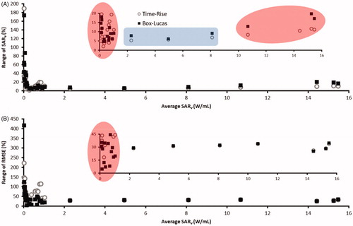
The range of the SAR_v and RMSE calculated with all start and evaluation time scenarios are shown in Figure 2, demonstrating the most stable results despite fitting method, for a SAR_v between 1 and 10 W/mL [19]. At low SAR_v (<1 W/mL) an increase in RMSE and SAR_v variation is observed, indicating the lower limit of SAR_v measurement (see red circle, Figure 2). The comparison of fitting parameters was challenging when SAR_v > 1.2 W/mL, due to the short duration (<30 s) removing the ability to evaluate the different evaluation times (30 s, 60 s, and full data range). The shortened timeframe results in a wider range in SAR_v for Box-Lucas than Time-Rise. The SAR_v range from 0.2–1.2 W/mL was selected to compare multiple evaluation times and adjust the starting point, because more data allowed for a comparison among all evaluation times. SAR_v did not show high variability (Supplemental Figures S1 and S2).

Figure 2. Effect of variation in SAR_v and RMSE using Box-Lucas and Time-Rise fitting as a function of SAR_v. Red circles indicate higher variation of SAR_v and RMSE caused by measurements performed in a sub-optimal heating range. The blue square indicates the range with a consistent SAR_v despite fitting method.

Figure 3(A,B) shows the impact of evaluation time on the variation of SAR_v and RMSE. Within this range of SAR_v values, it is observed that the Time-Rise fitting method is more sensitive than the Box-Lucas fitting method to the chosen evaluation time. This is expected since with increasing evaluation time the effect of heat loss on the dataset becomes noticeable and the assumed adiabatic assumption needed for Time-Rise is violated. More specifically within the dataset (Figures S1 & S2), we observed that the calculated SAR_v decreased while RMSE increased with increasing evaluation time. Therefore, SAR_v is underestimated when a long evaluation time which includes heat losses is selected. RMSE is more sensitive to heat losses caused by long evaluation times and can be used to select an appropriate evaluation time.

Figure 3. Evaluation and start time impact on SAR_v and RMSE. Plots A and B show the impact of evaluation time on SAR_v and RMSE when the start time is selected at 5s after heating. The SARv values are compared with the average SAR_v across all 12 fitting scenarios. A higher impact in both variation of SAR_v and RMSE is observed with Time-Rise fitting. Figure 3C evaluates the percentage difference in SAR between (1) SAR_v calculated excluding the first 5 s and (2) SAR_v calculated including t = 0-5 in the selected data range. Similarly, 3D evaluates the percentage difference in RMSE between these two cases. In this case, Box-Lucas fitting is observed to have larger variations in both SARv and RMSE than variations observed with Time-Rise fitting.

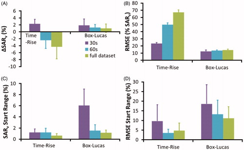
Figure 3(C,D) show Box-Lucas fitting to be more sensitive to start time than Time-Rise fitting. While not observed within this comparison, if the selection of the start time creates a dataset that includes the initial heating non-linear response, the SAR_v will be underestimated with Time-Rise fitting due to the decrease in the slope of the linear fit [14]. The Box-Lucas fitting method shows an increase in SAR_v and a decrease in RMSE (Figures S1 & S2) caused by selecting a start time that does not include the initial heating non-linear response (i.e. analysis is performed 5 s after the experimental start time). Therefore, when the timeframe selected incorporates data from the initial 5 s, inaccurate results are acquired. For Box-Lucas fitting, including the initial non-linear heating response causes a decrease in the exponential factor to fit the curvature of the temperature change as a function of time. For both Time-Rise and Box-Lucas fitting methods, the assumption is that heat is being deposited into the sample/system; the initial heating non-linear response indicates a timeframe where steady-state heat generation is not observed and should not be used for analysis. It is important to note the variation in SAR_v is relatively low (<10%) with changes in the evaluation time and start time; however, the effects of selecting the time frame of the dataset can be observed with the RMSE.

Finally, rigidly selected evaluation and start times were compared with automated selection methods for the evaluation time (R² optimization) and start time (quasi-adiabatic criteria). Both automated methods resulted in a reduction in RMSE (Figure S2). For the Time-Rise fitting method, the calculated SAR_v increased with increasing heat production when using R² optimization. The R² optimization was able to reduce the evaluation time to as short as 5 s, which allowed the dataset to comply with the adiabatic assumption of Time-Rise as experimental conditions (i.e. IONP, frequency, and magnetic field amplitudes) resulted in an increase of SAR_v. Therefore, the observed increase in SAR_v with a decrease in RMSE indicates a shortened dataset removing heat loss effects. R² optimization had negligible impact on SAR_v or RMSE calculated through the Box-Lucas fitting method. Furthermore, the use of the quasi-adiabatic selection for start time, did not have a significant effect on SAR_v or RMSE compared to the 5 s delay start time.

Case 2: Etheridge et al.

The range of the SAR_v and RMSE calculated with all start and evaluation time scenarios are in Supplemental Figure S3 [29]. The Etheridge et al. dataset demonstrated higher RMSE compared to the Bordelon et al., likely caused by the higher noise within the experimental setup. Similar to observations with Bordelon et al., higher variations in SAR_v based on fitting parameters were evident as SAR_v decreased, Time-Rise fitting results are more sensitive to evaluation time, and SAR_v calculated with Box-Lucas fitting is more sensitive to changes in start time. Evaluation of the full dataset time-interval caused Time-Rise SAR_v to be approximately 30% higher than the average SAR_v (Supplemental Figure S4) and RMSE to be over 350% higher than SAR_v (Supplemental Figure S5). The large effect on Time-Rise SAR_v and RMSE is caused by the 300 s evaluation time causing a violation of the adiabatic assumption.

Figure 4. Repeatability of SARv measurement. Plot A shows the standard deviation of the replicate measurements as a function of evaluation time (using 5s start time) for SAR_v ≤ 0.1 W/mL. Plot B right shows the standard deviation of the replicate measurement as a function of evaluation time for SAR_v ≥ 0.1 W/mL. An increase in variation is observed at lower SAR_v. Furthermore, the R2 optimization results in more variable results than a statistically set evaluation time.

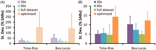
Very few datasets were observed to have RMSE <10% SAR_v (Supplemental Figure S5); however, the standard deviation of replicate measurements was <10% SARv with rigid time-frame selection (Figure 4). Although a very high RMSE (>500% SAR_v) was calculated for many datasets, this did not impact the repeatability of using the Time-Rise fitting for analysis. It is important to recognize that a high RMSE indicates a deviation from the assumptions of the fitting method. For Time-Rise fitting, as the SAR_v increases the heating losses become sufficient to violate the adiabatic assumption. Similarly, a violation of the linear heating losses assumption for Box-Lucas fitting should occur as SAR_v increases, although this was not observed for the range of SAR_v evaluated. Therefore, it is important to report RMSE to indicate the accuracy of the assumptions made with the fitting method used to calculate SAR_v and to report the standard deviation as an indication of the ability to repeat measurements.

Figure 4 demonstrates the impact evaluation time has the on repeatability of measurement, as well as the impact of using an automated method, such as the R² optimization for selecting the evaluation time. The selection of start time, resulted in the variations of the calculated SAR_v, however, no trend based on the start time selected is visible (Supplemental Figure S6). Furthermore, automating the start point selection using the quasi-adiabatic method did not result in an increased variation in the repeatability of the measurements. Within the datasets, five data points were removed as outliers using the Q-test for comparing SAR_v across the different fitting parameters. These outliers only occurred for automated fittings (both R² optimization and quasi-adiabatic selection). Additionally, the high noise within the discrete derivative was problematic and was removed by using a total-variation regularization [30]. The increase in this effect as SAR_v decreases indicates automated methods for selecting the dataset timeframe become less robust with increasing noise.

Table 1 summarizes recommendations for parameters to report for fitting with either linear-rise or Box-Lucas, depending on the range of SAR_v. Overall, the evaluation of RMSE, for a dataset and a fitting method (Time-Rise vs Box-Lucas) with its underlying assumptions, will help guide the selection of evaluation time and start time for that fitting method. Generally, while employing the Time-Rise fitting method, short time intervals (<30 s) that satisfy the quasi-adiabatic criteria are suitable for SAR_v estimation (small RMSE). Box-Lucas estimation, on the other hand, is less influenced by the length of the evaluation time interval, if losses in the system are linear. However, high SAR_v values (e.g. SAR_v >10 W/mL) can result in high RMSE using the Box-Lucas method because of non-linear losses in the measurement. In such cases, Time-Rise fit, constrained by the quasi-adiabatic criteria, can be a better fitting method. For both fitting methods, a target SAR_v range of 1-10 W/mL (specific to the datasets evaluated here), appears to generate consistent SAR_v values. An initial calibration of c(Fe) vs SAR_v across a broad range of iron concentration (e.g. 1-10 mg Fe/mL) may be useful to ascertain an optimal SAR_v range for a specific laboratory and setup. For both fitting methods, it is recommended to select a start time from the T vs t data that does not include the initial heating non-linear response (i.e. remove temperature data in the 0-5 s from the onset of heating in the fitting analysis). Additionally, reduction in peak-to-peak noise in the temperature measurement to ≤0.06 °C is desirable to reduce its contribution to the RMSE. Calibration of the AMF coil, calorimeter, temperature probes and the use of appropriate insulation are essential to characterizing and reducing the peak-to-peak noise.

Table 1. Recommended parameters to report^a.

SARv (W/mL)	Recommendation
< 1	For high noise, Time-Rise use RMSE to guide selection of the evaluation time, and report criteria used to select the time interval for analysis of heating data
	For low noise -> Either Method
1–10	Both methods work, report selected method and use RMSE to guide selection of evaluation time and start time
> 10	Box-Lucas, use RMSE to guide start time; expect inaccuracy if dataset is shortened due to physical sample constraints (i.e. boiling).

^aSAR_v ranges given are specific to Bordelon et al. & Etheridge et al. and will vary based on heating losses in the experimental setup.

The challenges of reliably comparing SAR_v across laboratories are related to the complex nature of the heat losses involved with the heating system and the sample. Most research findings report field strength, field amplitude, and sample information; however, many details related to the experimental setup are necessary to understand the heat losses within the system. Calibration of calorimeter, field properties, and other components of the apparatus are rarely performed, presenting significant challenges for comparisons absent standard reference materials. Additionally, the precision and accuracy with which the iron content is quantified will affect the calculated SLP. While ICP-MS is the gold-standard for iron quantification due to its sensitivity (ng/L detection limits), less expensive spectrophotometric assays have been optimized to measure iron content in 0.1–1μg/mL range [22,23], which should be suitable for SLP evaluation. Finally, the sample volume used for measurements has been shown to critically affect the results, likely due to heat transfer between sample and environment [27,28]. We recommend researchers report at least the experimental details listed in Table 2 to indicate the sample preparation and heat losses within an experimental setup. Finally, it cannot be overlooked that each experimental setup has an optimal range of SAR_v and adjustment of IONP concentration to be within that range can reduce variation results caused by fitting method.

Table 2. Recommended parameters to report.

Sample	Experimental setup	Calculation parameters	Reported calculations
Volume (≥ 2 mL) Sample holder Matrix (tissue, cells, or solution) IONP concentration [15] Method of cFe determination [22,23]	Coil (geometry and # of turns) [8,14,28] Temperature probe (type & placement) [14,16,17] Insulation Sample placement in coil [8,27] Magnetic field frequency Magnetic field amplitude Uniform field VOI	Fitting method Start point selection Evaluation time Number of replicate measurements	SARv or SLP RMSE of fit Standard deviation of replicate measurements

Conclusion

Valid selection between Time-Rise and Box-Lucas analysis for heating experiments depends on the experimental setup and the systematic error introduced in the calorimetric measurement. If a heating range appropriate for the apparatus is selected, where variation in reported SAR_v is minimal, the choice between parameters for analysis is within 10% of each other. For the experimental measurements evaluated here, this range was 1–10 W/mL. Recommendations for selecting between Time-Rise or Box-Lucas parameters are provided in Table 1.

Outside of the optimal SAR_v measurement range, a consistent analysis method can allow for repeatable SAR_v results, although accuracy is questionable. Selection of analysis methods and parameters can hardly compensate for poor quality data obtained. Proper calibration of calorimeter, thermometers, AMF field and frequency, etc. are absolute requirements for conducting such measurements. The assumptions of Time-Rise and Box-Lucas fitting should be considered when selecting evaluation time and start time, although the underlying cause of this is presently unclear. A decrease in RMSE can act as a helpful metric for comparing the selection of evaluation time or start time; however, automated methods optimized on minimizing RMSE can produce higher variations in results if a measurement is noisy. In short, these anomalies should be considered as indications that systematic (or systemic) errors exist in the measurement methods or apparatus, bearing a reexamination.

Acknowledgements

We thank Michael Etheridge for conversations related to the development of this manuscript.

Disclosure statement

R.I. is an inventor on nanoparticle patents, and all patents are assigned to either The Johns Hopkins University or Aduro BioTech, Inc. R.I. consults for Imagion Biosystems, a company developing imaging with magnetic iron oxide nanoparticles. R.I received partial funding from the National Cancer Institute (5R01CA194574-02 and 5R01CA247290). J.C.B. is an inventor on several patents that use iron oxide and gold nanoparticles to heat biomaterials for regenerative medicine purposes. These patents are assigned to the University of Minnesota. H.R., A.S. and J.C.B. received partial funding from NIH R01 HL135046 & R01 DK117425 which are related to iron oxide nanoparticle rewarming of vitrified biomaterials. J.C.B. was also supported by the Bakken Chair for Engineering in Medicine at the University of Minnesota. All other authors report no conflicts of interest. The contents of this paper are solely the responsibility of the authors and do not necessarily represent the official view of the Johns Hopkins University, University of Minnesota, NIH, or other funding agencies.

References

- Mahmoudi K, Bouras A, Bozec D, et al. Magnetic hyperthermia therapy for the treatment of glioblastoma: a review of the therapy’s history, efficacy and application in humans. Int J Hyperthermia. 2018;34(8):1316–1313.
- Ring HL, Bischof JC, Garwood M. The use and safety of iron-oxide nanoparticles in MRI and MFH. In Handbook – RF safety. Shrivastava D, editor. Hoboken, NJ: eMagRes;2019.
- Rosensweig RE. Heating magnetic fluid with alternating magnetic field. J Magn Magn Mater. 2002;252:370–374.
- Dennis CL, Jackson AJ, Borchers JA, et al. Nearly complete regression of tumors via collective behavior of magnetic nanoparticles in hyperthermia. Nanotechnology. 2009;20(39):395103.
- Giustini AJ, Ivkov R, Hoopes PJ. Magnetic nanoparticle biodistribution following intratumoral administration. Nanotechnology. 2011;22(34):345101–345101.
- Hoopes PJ, et al. Intratumoral Iron Oxide Nanoparticle Hyperthermia and Radiation Cancer Treatment. in SPIE Proceedings. 2007.
- Southern P, Pankhurst QA. Commentary on the clinical and preclinical dosage limits of interstitially administered magnetic fluids for therapeutic hyperthermia based on current practice and efficacy models. Int J Hyperthermia. 2018;34(6):671–686.
- Zhang J, Ring HL, Hurley KR, et al. Quantification and biodistribution of iron oxide nanoparticles in the primary clearance organs of mice using T1 contrast for heating. Magn Reson Med. 2017;78(2):702–712.
- Hoopes PJ, Petryk AP, Gimi B, et al. In Vivo imaging and quantification of iron oxide nanoparticle uptake and biodistribution. Proceedings of SPIE, 2012;8317:83170R.
- Chen R, Romero G, Christiansen MG, et al. Wireless magnetothermal deep brain stimulation. Science. 2015;347(6229):1477–1480.
- Manuchehrabadi N, Gao Z, Zhang J, et al. Improved tissue cryopreservation using inductive heating of magnetic nanoparticles. Sci Transl Med. 2017;9(379):eaah4586.
- Sharma A, Bischof JC, Finger EB. Liver cryopreservation for regenerative medicine applications. Regener Eng Transl Med. 2019 DOI:10.1007/s40883-019-00131-4
- Tong S, Quinto CA, Zhang L, et al. Size-dependent heating of magnetic iron oxide nanoparticles. ACS Nano. 2017;11(7):6808–6816.
- Wildeboer RR, Southern P, Pankhurst QA. On the reliable measurement of specific absorption rates and intrinsic loss parameters in magnetic hyperthermia materials. J Phys D: Appl Phys. 2014;47(49):495003.
- Lahiri BB, Ranoo S, Philip J. Uncertainties in the estimation of specific absorption rate during radiofrequency alternating magnetic field induced non-adiabatic heating of ferrofluids. J Phys D: Appl Phys. 2017;50(45):455005.
- Makridis A, Curto S, van Rhoon GC, et al. A standardisation protocol for accurate evaluation of specific loss power in magnetic hyperthermia. J Phys D: Appl Phys. 2019;52(25):255001.
- Skumiel A, Hornowski T, Józefczak A, et al. Uses and limitation of different thermometers for measuring heating efficiency of magnetic fluids. Appl Therm Eng. 2016;100(Supplement C):1308–1318.
- Soetaert F, Kandala SK, Bakuzis A, et al. Experimental estimation and analysis of variance of the measured loss power of magnetic nanoparticles. Sci Rep. 2017;7(1):6661.
- Bordelon DE, Cornejo C, Grüttner C, et al. Magnetic nanoparticle heating efficiency reveals magneto-structural differences when characterized with wide ranging and high amplitude alternating magnetic fields. J Appl Phys. 2011;109(12):124904.
- Hurley KR, Ring HL, Etheridge M, et al. Predictable heating and positive MRI contrast from a mesoporous silica-coated iron oxide nanoparticle. Mol Pharm. 2016;13(7):2172–2183.
- Zhang J, Chamberlain R, Etheridge M, et al. Quantifying iron-oxide nanoparticles at high concentration based on longitudinal relaxation using a three-dimensional SWIFT look-locker sequence. Magn Reson Med. 2014;71(6):1982–1988.
- Hedayati M, Abubaker-Sharif B, Khattab M, et al. An optimised spectrophotometric assay for convenient and accurate quantitation of intracellular iron from iron oxide nanoparticles. Int J Hyperthermia. 2018;34(4):373–381.
- Ring HL, et al. Ferrozine assay for simple and cheap iron analysis of silica-coated iron oxide nanoparticles. ChemRxiv. 2018.
- Etheridge ML, Hurley KR, Zhang J, et al. Accounting for biological aggregation in heating and imaging of magnetic nanoparticles. Technology (Singap World Sci). 2014;2(3):214–228.
- Teran FJ, Casado C, Mikuszeit N, et al. Accurate determination of the specific absorption rate in superparamagnetic nanoparticles under non-adiabatic conditions. Appl Phys Lett. 2012;101(6):062413.
- Landi GT. Simple models for the heating curve in magnetic hyperthermia experiments. J Magn Magn Mater. 2013;326:14–21.
- Huang S, Wang S-Y, Gupta A, et al. On the measurement technique for specific absorption rate of nanoparticles in an alternating electromagnetic field. Meas Sci Technol. 2012;23(3):035701.
- Wang SY, Huang S, Borca-Tasciuc DA. Potential sources of errors in measuring and evaluating the specific loss power of magnetic nanoparticles in an alternating magnetic field. IEEE Trans Magn. 2013;49(1):255–262.
- Etheridge ML, Bischof JC. Optimizing magnetic nanoparticle based thermal therapies within the physical limits of heating. Ann Biomed Eng. 2013;41(1):78–88.
- Chartrand R. Numerical differentiation of noisy, nonsmooth data. ISRN Appl Mathematics. 2011;2011:1–11.
- Bordelon DE, Goldstein RC, Nemkov VS, et al. Modified solenoid coil that efficiently produces high amplitude AC magnetic fields with enhanced uniformity for biomedical applications. IEEE Trans Magn. 2012;48(1):47–52.
- Conde-Leborán I, Serantes D, Baldomir D. Orientation of the magnetization easy axes of interacting nanoparticles: influence on the hyperthermia properties. J Magn Magn Mater. 2015;380:321–324.
- Munoz-Menendez C, Conde-Leboran I, Baldomir D, et al. The role of size polydispersity in magnetic fluid hyperthermia: average vs. local infra/over-heating effects. Phys Chem Chem Phys. 2015;17(41):27812–27820.
- Engelmann UM, Shasha C, Teeman E, et al. Predicting size-dependent heating efficiency of magnetic nanoparticles from experiment and stochastic Néel-Brown Langevin simulation. J Magn Magn Mater. 2019;471:450–456.