Evaluation of a numerical simulation for cryoablation – comparison with bench data, clinical kidney and lung cases

Abstract

Purpose

The accuracy of a numerical simulation of cryoablation ice balls was evaluated in gel phantom data as well as clinical kidney and lung cases.

Materials and methods

To evaluate the accuracy, 64 experimental single-needle cryoablations and 12 multi-needle cryoablations in gel phantoms were re-simulated with the corresponding freeze-thaw-freeze cycles. The simulated temperatures were compared over time with the measurements of thermocouples. For single needles, temperature values were compared at each thermocouple location. For multiple needles, Euclidean distances between simulated and measured isotherms (10 °C, 0 °C, −20 °C, −40 °C) were computed. Furthermore, surface and volume of simulated 0 °C isotherms were compared to cryoablation-induced ice balls in 14 kidney and 13 lung patients. For this purpose, needle positions and relevant anatomical structures defining material parameters (kidney/lung, tumor) were reconstructed from pre-ablation CT images and fused with postablation CT images (from which ice balls were extracted by manual delineation).

Results

The single-needle gel phantom cases showed less than 5 °C prediction error on average. Over all multiple needle experiments in gel, the mean and maximum isotherm distance were less than 2.3 mm and 4.1 mm, respectively. Average Dice coefficients of 0.82/0.63 (kidney/lung) and mean surface distances of 2.59/3.12 mm quantify the prediction performance of the numerical simulation. However, maximum surface distances of 10.57/10.8 mm indicate that locally larger errors have to be expected.

Conclusion

A very good agreement of the numerical simulations for gel experiments was measured and a satisfactory agreement of the numerical simulations with measured ice balls in patient data was shown.

Keywords:

• Cryoablation
• numerical simulation
• lung
• kidney
• evaluation

Introduction

Cyroablation is a minimally invasive ablation procedure used to treat patients when surgery is not possible due to general patient’s health conditions, difficult accesses, or multiple scattered lesions [1,2]. During cryoablation, one or multiple cryoprobes [3–5] – needle-shaped instruments – are inserted into the target structure in order to cool the tissue below its freezing point. In clinical practice, several freeze-thaw cycles are applied sequentially [6–8]. The target cells are damaged during the freeze-thaw cycles as a result of several processes [9] such as crystallization of water, cell dehydration, metabolic derangement and vascular stasis [9]. Cooling rate and temperature significantly influence the tissue damage due to the differences in intra- and extracellular ice formation which result in osmotic tension between intra- and extracellular space and cell dehydration [10]. The majority of cryoablation treatments are performed on the prostate, bone, breast, pancreas [11], but also kidney [12] and lung [13]. To improve the ablation volume, combinations of cryoablation with the injection of liquids with other thermal properties [14], and with immunotherapies [15,16] have been proposed. For more details on cryoablation, we refer to the reviews [1,2].

For a successful ablation, it is important to create a sufficiently large damage zone enclosing the complete target tumor. The required target temperature and ablation time, that is, time for which the target temperature has to be reached, is subject to discussion in the scientific literature [9]. Thus, this paper focusses on the comparison of the simulated and measured temperatures, without comparing simulated and measured necrosis. The mapping between the space–time temperature evolution and tissue damage will be handled in subsequent work and has no influence on the temperature validation.

Depending on target location and size, several cryoprobes have to be inserted simultaneously to reach complete destruction of the ablation target. In clinical practice, the operator has to determine needle placements using the expected ice ball dimensions given by the manufacturers of the cyroablation devices, which are obtained based on animal studies or benchmark ablations in gel phantoms. To improve therapy planning, patient-specific numerical simulations have been introduced in the last decades [1]. Rossi and Rabin et al. [17,18] proposed efficient numerical approaches to experimental validation of cryosurgery. Keelan et al. [19] investigated bioheat simulation for cryoablation using the graphics processing unit (GPU). Furthermore, they investigated the use of the proposed simulation as a training tool. Another training tool aimed at prostate cryosurgery has been presented by Rabin et al. [20]. Zhang et al. [21] discussed numerical simulation for heat transfer of cryoablation in prostate cancer.

Most of the papers mentioned above presented new approaches for modeling cryoablation but did not validate the results against real ablations. Zhang et al. [22] and Hossain et al. [23] modeled multi-probe cryoablations and both compared simulated results to phantom data by Shaikh et al. [24]. Temperatures measured with thermocouples in gel phantoms are discussed by Ramajayam et al. [14]. Zhang et al. [25] simulated the effects of an MRI-compatible cryoprobe and compared numerical results to their own measurements. Golkar et al. [26] presented a GPU-based modeling for fast cryoablation simulation. They compared their results with the work of Shah et al. [27] who used a thermocouple matrix structure to measure temperatures in an ultrasound gel phantom and validated Golkar’s results on five patient cases using intraoperative MRI images.

In this paper, we report on the evaluation of the accuracy of a previously published numerical simulation method which allows to calculate the temperature of cryoablations [13]. We performed numerical validation experiments to analyze the impact of uncertainty in simulation parameters on the simulation results. Additionally, we compared the resulting temperatures at spatial positions as well as temperature isotherms of numerical simulations to experimental single-needle and multi-needle cryoablations in gel phantoms. Finally, we evaluated the accuracy of the simulation method in a clinical setting by comparing simulated ice balls with ice balls from patient lung and kidney cryoablations.

Materials and methods

Numerical model

The numerical model [13] evaluated here takes into account the phase change process [28], an effective conductivity model [29], and state-dependent material parameters: (1) $$\frac{\partial }{\partial t}\left(\rho cT\right)=\nabla ·\left(k_{\text{eff}}\nabla T\right)-l\Lambda \frac{\partial }{\partial t}\left(\rho \left(1+F\right)\right).$$(1)

In this equation, the density $\rho ,$ the heat capacity $c,$ and the effective conductivity $k_{\text{eff}}$ are state-dependent, i.e. they change with the temperature $T.$ We use a piecewise linear parameter model that continuously interpolates the parameters based on fixed parameter values given at sampling points, that is, at various temperatures $T_i.$ The latent heat resulting from the phase changes between liquid water and ice are modeled via a mushy region approach, that is, the amount of ice represented by the mushy region variable $F$ may be any number in $\left[-1,0\right],$ where −1 represents a fully frozen state. Since the organs of interest are composed of different materials, the model takes into account the relative water content $\Lambda$ and the mass specific latent heat $l.$ The latent heat or enthalpy of fusion has a significant influence on the temperature distribution. It represents the energy that is required to transform a unit mass of ice into water at constant pressure. This energy is absorbed by the mass without changing its temperature but stored as internal energy, due to the fact that liquid water has weaker intermolecular forces than solid ice and thus a higher potential energy. When the state changes from liquid water to solid ice, the energy stored as latent heat is released.

The continuous model was discretized by using an explicit time stepping scheme and by using a regular and isotropic hexahedral grid. This allows to massively parallelize the calculations using a single instruction multiple data architecture (graphical processing units).

Further details regarding the numerical model, the discretization, and the numerical implementation are given in [30].

Numerical validation

To quantitatively analyze the impact of uncertainty in model parameters on the simulation results, a sensitivity analysis was performed.

For this purpose, two classes of simulation parameters were considered: patient-associated parameters (tissue material properties, body temperature as initial and boundary condition) and a therapy-associated parameter (needle temperature).

There are two sources of uncertainty in the patient-associated parameters:

• Variations on an individual basis, for example, between different patients, because the patient-associated parameters are based on population averages and do not take inter-patient variations into account.

• Variations reported in the literature. There are various material parameter studies reported in the scientific literature and the numerical simulation uses patient-associated parameters aligned with the parameter ranges reported in the literature. However, we restrict the analysis to uncertainty in the parameters of the tissue parameter models and do not take uncertainty with respect to the chosen parameter model into account.

Both uncertainty sources for the patient-associated parameters have to be taken into account when using or analyzing the numerical simulation result.

This sensitivity analysis used ranges of material parameters reported in the literature, in most cases based on the ITIS tables [31]. There are very few publications dealing with state-dependent material parameter models. Thus, deriving a state-dependent model that can be used for sensitivity analysis is not directly possible. Instead, a simplified model for the parameter variations was used here: from the material parameter used in the simulation at body temperature, that is, at T_body = 310.15 K, the percentage deviation between this parameter and the parameter ranges reported in the ITIS tables were computed. For example, for a parameter α_Sim, the relations α_{rel min} = α_{min ITIS}/α_Sim(T_body) and α_{rel max} = α_{max ITIS}/α_Sim(T_body) were computed. Based on this relative parameter uncertainty, the state-dependent material parameters were rescaled using a uniform sampling in the interval I= [α_{rel min},α_{rel max}] to α_sensi(T)=α_rel · α_Sim(T) for a α_rel ∈I. Ranges for the patient-associated and therapy-associated parameter values are listed in Table 1.

Table 1. Parameter values used in the sensitivity analysis for kidney and lung tissue.

		Kidney			Lung
Parameter name	Unit	Min	Max	Default	Min	Max	Default
Density	kg m^3	1019	1147	1066	255	1050	722
Heat capacity	J kg^−1 K^−1	3505	3891	3505	3653 38	4119	3886
Thermal conductivity	J m^−1 s^−1 K^−1	0.499	0.56	0.55	0.2495	0.4957	0.275
Relative Blood Perfusion Rate	s^−1	0.0044	0.0888	0.071	0.00173	0.007	0.0048
Body temperature	°C	35.5	38	37	35.5	38	37
Needle temperature	°C	−180	−119.15	−143.15	−180	−119.15	−143.15

Using an equidistant sampling of [α_{rel min},α_{rel max}], corresponding to a uniform distribution of α_rel, treatment cycles were then simulated with a setup consisting of a single needle in homogeneous kidney or lung tissue. From the final temperature distribution, a temperature profile along a radial axis orthogonal to the needle was generated.

These radial temperature profiles were plotted to provide an overview of the sensitivity of the simulation results to uncertainty in the patient-associated parameters. As a quantitative measure, the maximal temperature difference was computed over all patient-associated parameter samples and spatial sampling points. Moreover, using the default values of the patient-associated parameters used by numerical simulation as a reference, mean and standard deviation of the differences of the temperature profiles to the reference for different ranges of temperatures were determined.

In a first step, each patient-associated parameter value was varied independently, keeping the remaining parameters at their respective default value. This approach identified those parameters that lead to highest uncertainty in the resulting temperature profiles. In a second step, the bivariate combination of the two parameters with highest sensitivity was investigated.

Gel phantom

To analyze the performance of the needles used in this study, gel phantom experiments testing different needle types while measuring the resulting temperatures at a multitude of positions relative to the needles with arrays of thermocouples over time have been performed by Shah et al. [11]. We used the measured data of these experiments in this work to assess the accuracy of the numerical simulation. As such, all conclusions drawn are only valid for cryoablation in the specific gel with the specific standardized cooling procedure of 10 min cooling, 5 min passive thawing, followed by another 10-min cooling.

Experiments were conducted with single needles or with multiple needles of the same kind used simultaneously. In all experiments the standard cooling cycle was performed. In single-needle experiments, a single-needle thermocouple (TC) matrix was used, see Figure 1(a) while for experiments with multiple needles the multi-needle TC matrix was used, see Figure 1(b).

Figure 1. Thermocouple matrices used for measuring the experiments. Figure a) shows thermocouple positions (+) for single needle assessment. The needle (red) is in-plane with the thermocouples. Figure b) shows thermocouple positions (+) for experiments with multiple needles. Slots in which the needles can be put are marked with circles (o), the needle is thus orthogonal to the measurement slice.

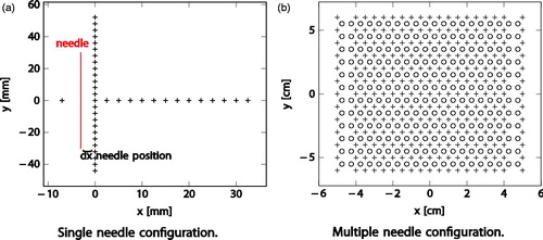
The multi-needle TC matrix fixture is an advanced TC fixture which enables the recording of the gel temperature in a plane corresponding to the largest ice ball diameter created by a set of needles used simultaneously. The fixture is comprised of 247 TCs in a grid pattern which enables the recording of the gel temperatures in 2.5 mm increments in the parallel direction and 5 mm in the perpendicular direction. A needle grid of 20 × 12 holes is assembled on top of the TCs array with a space of 10 mm in the y axis and 5 mm on the x axis. A sketch of the TCs together with the grid needle slots locations is shown in Figure 1(b). A more detailed description of the experimental setup can be found in the work of Shah et al. [11].

Single needle

For the single-needle cases, the temperature profiles parallel and perpendicular the needle at the end of both the first and second cooling cycle were analyzed. We restrict the analysis to the end of the freezing cycles because clinical patient data is available for the end of the freezing cycle only. Once temporally resolved clinical temperature data, e.g. from MR-based cryo-thermometry [DOI: 10.1002/jmri.25301], is available, the analysis could be extended to the whole freeze-thaw cycle. This would enable investigations of effects like primary and secondary ice fronts.

For each experiment, the following data were used as input for the numerical simulation:

• gel temperature at experiment start,

• measured needle distance from thermocouple line parallel to needle, (dx in Figure 1(a)),

• the used thermocouple matrix with positions of the thermocouples,

• the time for which the analysis should be performed.

The simulation was performed on a 100 mm × 120mm × 100mm grid with 1 mm isotropic voxel size. The needle was located at x = 0 and the thermocouple positions were moved by the measured needle distance in direction of the positive x-axis. The temperature at all thermocouple positions was read from the simulated temperature distribution and comparisons were computed only for these virtual thermocouple readings. To compare the simulated temperature to the measurements, we computed average errors for multiple temperature ranges: that is for each pair of simulated temperature T_sim and measured temperature T_actual, we first determined in what analysis range T_actual is and then added the error T_sim−T _actual to the samples within that range. For each temperature range, we then determined the average error and the standard deviation in °C. In case of only a single sample within a certain range, the standard deviation is zero. In case of no samples within a certain range, both the average value and standard deviation are zero. The analyzed temperature ranges were defined as [−∞, −45), [−45, −35], (−35, −25), [−25, −15], (−15, −5), [−5, 5].

Multiple needles

For experiment with multiple needles, the cryoablation device manufacturer provided isotherms for −40 °C, −20 °C, 0 °C, and 10 °C. To compute the isotherms, in a first step, the raw data at the specific time for all thermocouples of the Multi-Needle TC Matrix was interpolated to an image grid (120 mm × 140 mm, 1 mm × 1 mm pixel size) using uniform B-splines. Afterwards, the isotherms were extracted from the 2 D image. An example case of two needles is shown in Figure 6. The white contours are the resulting contours of our recalculation based on the raw data, while the black contours are the contours provided by the cryoablation device manufacturer. Small differences in the isotherms result from different interpolation and contour computation tools used by the cryoablation device manufacturer.

For each experiment with multiple needles, the following data were used as input for the setup of the numerical simulation:

• gel temperature at experiment start,

• needle positions for all needles,

• the thermocouple matrix with positions of the thermocouples, and

• the time for which the analysis should be performed.

Again, the simulation was performed on a 100 mm × 120mm × 100mm grid with 1 mm isotropic voxel size. The temperature at all thermocouple positions was read from the simulated temperature distribution and temperature differences were computed only for these virtual thermocouple readings. The isotherms were computed directly from the simulated temperature distribution, i.e. not from the interpolated virtual thermocouple readings. This approach has the benefit of implicitly verifying that the B-spline interpolation used to compute a dense temperature distribution and isotherms from the sparse thermocouple measurements is suitable and that the sparse thermocouple distribution is dense enough to describe the relevant isotherms.

In addition to the temperature binning that was already assessed for the single-needle experiments, we assessed contour distances for the multiple needle experiments. We computed the minimum, maximum, and mean of the distances for each isotherm. The distances were computed for each discrete point of the ground truth contour C_gt by evaluation D(x,C_candidate): = min{d(x, k) | k ∈ C_candidate} with d(a, b) being the Euclidean distance in mm.

Clinical kidney and lung data

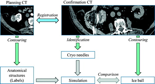
Because the biophysical material properties of gel substantially differ from in-vivo tissue and because the needle positions are not always parallel, the validation of gel phantoms cannot be transferred to patients. Thus, we compared 0 °C isotherms computed with the numerical simulation with ice balls from clinical kidney and lung cryoablations. For this purpose, relevant anatomical structures were contoured from planning CT images in order to apply the corresponding material parameters to labeled tissue types. The labels are background, kidney/lung, and tumor. Based on the intra-interventional confirmation CT image, needle positions were extracted from the visible needles and the ice balls have been contoured. To compensate for anatomical deformations and patient movements, both CT data sets were co-registered by a rigid transformation so that needles and ice balls are at the correct spatial position with respect to the planning CT.

The anatomical structures mentioned above were contoured on planning CT images using a manual slice-by-slice contouring procedure. The ice balls were contoured with the same method from confirmation CTs which were acquired immediately after the ablation was finished with inserted needles. For the kidney cases, the ice balls appear as regions of lower contrast compared to surrounding anatomical structures, but for the lung cases with higher contrast. To spatially register the corresponding images, a manual rigid co-registration method was used. The cryoablation needles were reconstructed by placing spatial positions for each needle tip and skin entry point in the intra-interventional CT images. All tasks were performed by experienced medical personnel. An overview of the image processing workflow can be found in Figure 2.

Figure 2. Overview of the annotation workflow for structure contouring, image registration, and needle identification. Image data sets are courtesy of Dr. Alex King, University Hospital Southampthon.

Only the front between ice and water is visible in CT images, so the temperature of the ice ball cannot be measured. To allow a comparison with the numerical simulation, we assume that the visible ice ball boundary has a temperature of 0 °C. This assumption is motivated by the work of Permpongkosol et al.³² who measured the temperatures during CT guided renal cryotherapy with thermocouples and suggest that the edge of the low-attenuation area likely represents 0 °C. Thus, the simulated 0 °C isotherm was compared with the contoured ice ball boundary for each case. Additionally, the corresponding elliptical ablation zones reported in the instructions for use by the ablation device manufacturer were compared with the contoured ice ball. The following measures were subsequently calculated in 3 D space:

• Dice coefficient,

• Relative volume error,

• Max surface distance, and

• Mean surface distance.

Results

Numerical validation

For univariate sensitivity analysis, the respective ranges of patient-associated parameters and initial conditions were calculated for steps of 5%, that is, in 21 equidistant steps. The parameter ranges are listed in Table 1. The distributions of the resulting temperature profiles are plotted in Figure 3.

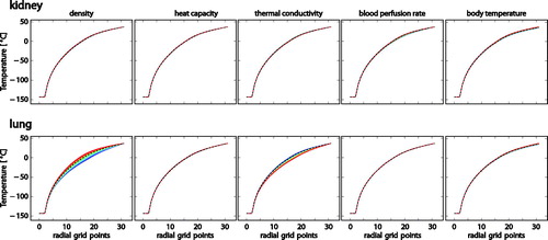
Figure 3. Plots showing the sensitivity to density, heat capacity, thermal conductivity, blood perfusion rate, and body temperature for kidney and lung, respectively. Line colors encode the parameter value according to a rainbow color map (blue: smallest, red: largest value considered, dashed black line: default value.

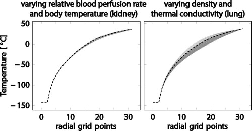
A bivariate sensitivity analysis was based on the results of the univariate analysis. For each organ, two patient-associated parameter values were identified for which the results are most sensitive. For kidney, relative blood perfusion rate and body temperature were most sensitive, for lung, density and thermal conductivity. The two parameter values were then varied simultaneously, where the two-dimensional range of parameters was now sampled with 11 equidistant points per parameter. As a result, the analysis shows a maximal temperature variation of 5.451 K for kidney and 21.735 K for lung (see Figure 4).

Figure 4. Bivariate sensitivity analysis for kidney tissue, varying relative blood perfusion rate and body temperature (left). Bivariate sensitivity analysis for lung tissue, varying density and thermal conductivity (right). The gray lines show the temperature profiles for the variation of the parameter values, the dashed black line corresponds to the default values.

Gel phantom

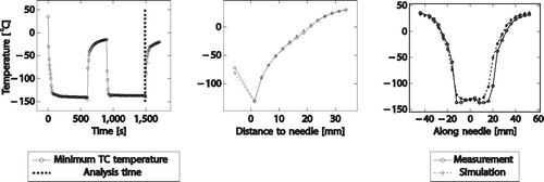
Figure 5 shows a result of the simulation for a cryo needle (IceFORCE^®, BostonScientific) at the end of the second cooling cycle compared to the measured temperatures for a single-needle experiment. The left plot shows the measured temperature over time and illustrates the analysis time. The middle plot shows measured and simulated temperature at each thermocouple perpendicular to the needle. The right plot shows the measured and simulated temperature along the needle.

Figure 5. Exemplary plot showing the simulated temperature at the end of the second cooling cycle compared to the temperature measurements (left: minimum temperature over time, middle: simulated vs. measured temperature perpendicular to needle, right: simulated vs. measured temperature along needle).

A total of 22 IceFORCE^®, 22 IcePEARL^®, 10 IceROD^®, and 10 IceSPHERE^® simulations was computed. The binned temperature differences over all 64 single-needle experiments comparing simulated temperature to measurements are given in the Table 2.

Table 2. Temperature differences over all single needle experiments comparing simulated temperature to measurements.

Temp Range [°C]	Avg Diff [°C]	std dev
(5, ∞]	1.82	1.67
[−5, 5]	5.11	3.66
(−15, −5)	4.81	4.22
[−25, −15]	4.11	3.69
(−35, −25)	4.90	3.55
[−45, −35]	4.45	3.89
[−∞, −45)	7.99	7.83

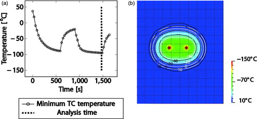
The result, at the end of the second cooling cycle, from two IceFORCE^® needles are shown in Figure 6 where (a) shows the minimum temperature over time plot with marking of the analysis time, (b) shows the simulated temperature distribution with isotherms overlaid (white: simulated, black: measured).

Figure 6. Exemplary results for a double-needle case. Left: measured temperature over time, right: overlay of simulated (white) and measured (black) isotherms on top of heat map.

Moreover, 12 multi-needle simulations were computed, for each needle type (IceFORCE^®, IcePEARL^®, IceROD^®, and IceSPHERE^®) two, three and four needles are placed in parallel. The temperature differences over all 12 multi-needle experiments are given in the Table 3.

Table 3. Temperature differences over all multi needle experiments comparing simulated temperature to measurements.

Temp Range [°C]	Avg Diff [°C]	std dev
(5, ∞]	1.18	1.31
[−5, 5]	6.42	3.93
(−15, −5)	6.96	4.36
[−25, −15]	5.05	3.47
(−35, −25)	6.22	3.42
[−45, −35]	5.55	4.24
[−∞, −45)	6.43	4.68

The overall contour distances of simulated isotherm contours to ground truth isotherm contours taking the respective metric over all experiments (average minimum, maximum, or mean surface distance over all experiments) are listed in Table 4.

Table 4. Overall contour distances for experiments with multiple needles.

Temperature °C	Minimum Surface Distance [mm]	Maximum Surface Distance [mm]	Mean Surface Distance [mm]
−40	0.002	3.29	1.21
−20	0.001	3.28	1.28
0	0.002	3.74	1.52
10	0.755	4.14	2.28

In addition, the grid size was varied for a simulation run and the results were plotted at two time steps. The original domain size of the experiments was 100 × 120 × 100 mm³. To assess the spatial convergence, the computations were performed on varying grids starting from 75 × 90 × 75 voxels refining four times with factor 1.3 up to 177 × 233 × 177 voxels (see Figure 7).

Figure 7. Spatial (left) and temporal (right) convergence in a gel phantom.

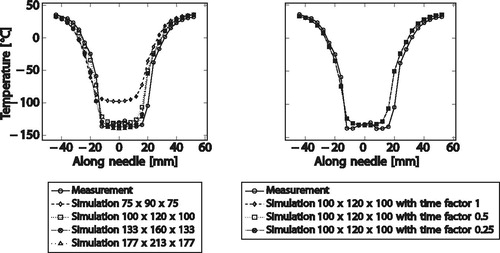
For the temporal convergence, the time step size was varied by a time factor for a simulation run and the results are plotted. The numerical simulation is usually computed on the native grid size [13], that is, with a time step size of 1.0. To ensure that the results do not vary substantially with a smaller time step size, we used time factors of 0.5 and 0.25 to assess the temporal convergence.

Clinical data

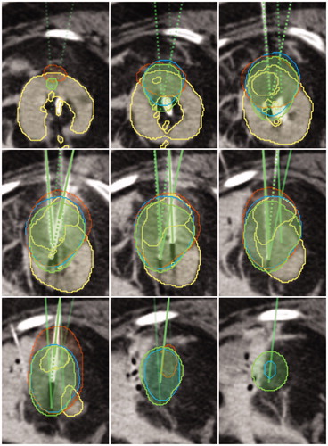
An example post-interventional kidney case is shown in Figure 8. Overlays show the contoured labels (yellow), the simulation result 0 °C isotherm (blue), the contoured ice ball (orange), as well as the needles with corresponding ellipsoids (green) as provided by the manufacturer. It can be seen that the numerical simulation has a better overlap compared to the ellipsoids.

Figure 8. Exemplary kidney case showing the contoured labels (yellow), the simulation result 0 °C isotherm (blue), the contoured ice ball (red), as well as the needles with corresponding ellipsoids (green). Image data sets are courtesy of Dr. Alex King, University Hospital Southampthon.

Averaged measures from 14 kidney cases including mean and standard deviation are shown in Table 5. The ellipsoid reported from the vendors needle specification as well as the numerical simulation were compared to the ice ball extracted from post-interventional image data. Averaged measures from 13 lung cases are shown in Table 6.

Table 5. Averaged measures of the kidney cases. (mean values and standard deviation over all cases).

Region(s)	Measure	Mean	Stdev
Ellipsoid–ice ball	Dice coefficient [0…1]	0.79	0.06
	Max surface distance [mm]	12.32	3.87
	Mean surface distance [mm]	3.05	0.90
	Relative volume error	0.19	0.13
Ellipsoid	Max 3 D diameter [mm]	59.42	9.52
	Volume [ml]	67.73	29.30
Ice ball	Max 3 D diameter [mm]	62.49	11.79
	Volume [ml]	69.45	36.86
Simulation–ice ball	Dice coefficient [0…1]	0.82	0.06
	Max surface distance [mm]	10.57	3.47
	Mean surface distance [mm]	2.59	0.97
	Relative volume error	0.18	0.12
Simulation	Max 3 D diameter [mm]	55.03	9.41
	Volume [ml]	65.52	31.79

Table 6. Averaged measures of the lung cases (mean values and standard deviation over all cases).

Region(s)	Measure	Mean	Stdev
Ellipsoid–ice ball	Dice coefficient [0…1]	0.50	0.17
	Max surface distance [mm]	12.24	3.52
	Mean surface distance [mm]	5.22	1.82
	Relative volume error	2.62	2.69
Ellipsoid	Max 3 D diameter [mm]	41.78	5.68
	Volume [ml]	26.72	5.68
Ice ball	Max 3 D diameter [mm]	41.80	10.46
	Volume [ml]	10.57	5.83
Simulation–ice ball	Dice coefficient [0…1]	0.63	0.13
	Max surface distance [mm]	10.80	5.81
	Mean surface distance [mm]	3.12	1.15
	Relative volume error	0.70	0.91
Simulation	Max 3 D diameter [mm]	32.63	5.17
	Volume [ml]	9.82	3.39

Discussion

Univariate sensitivity

The univariate sensitivity of the temperature profiles to patient-associated parameter uncertainty is generally small (a few Kelvins, see Figure 3), except for the sensitivity to density of the lung tissue and the thermal conductivity of lung tissue. This is plausible because most patient-associated parameter values have been reported in fairly narrow ranges in the literature, thus the resulting temperature can also be expected not to vary substantially. Lung tissue density and thermal conductivity, however, were varied over a broad range of literature values, and the resulting temperature values vary accordingly.

The largest temperature differences occur near the freezing point of water for most of the patient-associated parameters, except for the relative blood perfusion rate and the body temperature. These observations are plausible because the phase change between liquid and frozen water requires large changes of energy for small changes of temperature, hence the largest impact of most of the parameters (which ultimately influence the heat transfer) can be expected near this temperature. Blood perfusion, in contrast, only happens in a temperature range between the freezing point and body temperature (37 °C), so changes in the blood perfusion rate can be expected to have most impact in this temperature range. The body temperature is used both as initial and boundary condition, so the variation of body temperature has highest impact at the boundary (lung) or near the boundary (kidney), where the dependency of interior material parameters slightly amplifies the impact of variable body temperature.

Multivariate sensitivity

The bivariate sensitivity for kidney and lung is smaller than the sum of the univariate sensitivities to the respective parameters. Similarly, the largest temperature differences are observed in the range between the two temperatures with largest differences from the univariate analysis.

These observations are plausible because no substantial additional sensitivity is expected from the interaction of varying more than one patient-associated parameter. The observations also suggest that the multivariate sensitivity to the uncertainty in all patient-associated parameters can be expected to be in the same range and not introduce substantial additional uncertainty of the simulated temperature profiles.

Gel phantom

Table 2 shows that for all single-needle temperature ranges except one, the temperature difference between ground truth measurements and simulated temperature are, on average, less than 5 K. This value is less than the reported deviations of the temperature defining lethal damage in the scientific community. The only range that exceeds this threshold is the range below −45 °C which is very close to the needle and thus highly influenced by grid resolution and needle discretization.

The spatial convergence analysis shows that 1 mm voxel sizes are suited for the simulations. Choosing a coarser grid with only 75 × 90 × 75 voxels with 1.3 mm × 1.3 mm ×1.3 mm voxel results in considerably larger errors while the 1 mm voxel results in predictions close to finer grid solution as well as the measurements. The temporal convergence analysis shows no considerable benefit of choosing smaller time steps than the largest possible time step fulfilling the stability criterion for the simulations.

Table 3 shows average differences less than 6.9 K for multiple needles—which, given the large range of temperatures, is considered an acceptable error. The contour distances in Table 4 show that this temperature error results in less than 4.1 mm isotherm location error. The mean contour distance is below 1.51 mm for the −40 °C, the −20 °C, as well as the 0 °C isotherm. The less important 10 °C isotherm shows a larger location error but is still below 2.28 mm.

As described previously in the single needle convergence analysis, the spatial convergence analysis shows that the 1 mm voxel size for the 100 × 120 × 100 voxel grid is a suitable resolution and there is only a small gain from choosing a finer resolution. There is no benefit of using smaller time steps than the stable time step.

Clinical cases

With an average Dice coefficient of 0.82/0.63 (kidney/lung) and a mean surface distance of 2.59/3.12 mm (kidney/lung), the results show that the prediction performance of the numerical simulation ranges is within the clinically accepted safety margin [33] of 5 to 6 mm. The maximum surface distance of 10.57/10.8 mm (kidney/lung) indicates that locally larger errors should be expected. Besides the uncertainties of the numerical models, various sources of errors are introduced in this validation.

Firstly, during the ablation procedures, the tissue of the target area is strongly deformed by inserting the needles. This deformation could only in part be compensated for by the rigid transformation between the pre-interventional planning and intra-interventional confirmation CT images. Thus, depending on the specific case, a large registration error of the order of several millimeters may to be expected.

Secondly, the medical experts faced several difficulties in the annotation of the ice balls. In some regions, the ice balls are hardly distinguishable from the surrounding tissue due to insufficient image contrast or high image noise. Furthermore, artifacts caused by metal in the cryoablation needles interfere with the expected Hounsfield units of the ice balls, resulting in boundaries which were difficult to distinguish.

Thirdly, the resolution of the image data itself is limited. The average in-plane resolution is 0.84/0.7 mm (kidney/lung) and the average slice thickness is 1.79/1.33 mm (kidney/lung).

Fourthly, within the limited number of clinical cases, a high inhomogeneity can also be observed. The number of needles and thus the size (maximal 3 D diameter and volume) of the ice balls differ substantially, which makes a statistical comparison difficult.

With respect to the given errors from registration and contouring of the clinical CT images, as well as the uncertainties in the numerical models, the results show a good agreement between the simulations and the measured ice balls. The simulations provide a better prediction of outcome that than the ellipsoids provided by the manufacturers.

Since the temperature of the ablation region cannot be measured in patients, we assume the visible ice ball represent the 0 °C isotherm. In order to improve the numerical simulation, an accurate damage model has to be developed and will be validated in future work.

Conclusions

Despite inter-individual variation and uncertainty of material parameters for lung and kidney tissue, simulated temperature profiles agree well with measured data: differences are a few Kelvins in gel phantom temperatures and below the range of surgical safety margins in clinically observed ice balls. Accurate numerical simulation were performed at spatial and temporal resolutions for which real-time computational performance [13] was achieved. This sufficiently accurate and fast pre-interventional prediction of ice balls is an important step toward a clinically applicable cryoablation planning system.

Acknowledgements

We would like to thank Galil Medical (Boston Scientific) for providing the bench data and clinical data used in this study. Furthermore, we would like to thank our colleagues Christiane Engel and Andrea Koller for contouring the clinical images, as well as David Sinden for proofreading the manuscript.

Disclosure statement

No potential conflict of interest was reported by the author(s).

References

- Rubinsky B. Cryosurgery. Annu Rev Biomed Eng. 2000;2(1):157–187.
- Yiu W, Basco MT, Aruny JE, et al. Cryosurgery: A review. Int J Angiol. 2007; 16(1):1–6.
- Keanini RG, Rubinsky B. Optimization of multiprobe cryosurgery. ASME. J. Heat Transfer. November 1992; 114(4):796–801.
- Baissalov R, Sandison GA, Donnelly BJ, et al. A semi-empirical treatment planning model for optimization of multiprobe cryosurgery. Phys Med Biol. 2000;45(5):1085–1098.
- Giorgi G, Avalle L, Brignone M, et al. An optimisation approach to multiprobe cryosurgery planning. Comput Methods Biomech Biomed Engin. 2013;16(8):885–895.
- Woolley ML, Schulsinger DA, Durand DB, et al. Effect of freezing parameters (freeze cycle and thaw process) on tissue destruction following renal cryoablation. J Endourol. 2002;16(7):519–522.
- Mala T, Edwin B, Tillung T, et al. Percutaneous cryoablation of colorectal liver metastases: potentiated by two consecutive freeze-thaw cycles. Cryobiology. 2003;46(1):99–102.
- Hinshaw JL, Littrup PJ, Durick N, et al. Optimizing the protocol for pulmonary cryoablation: a comparison of a dual- and triple-freeze protocol. Cardiovasc Intervent Radiol. 2010;33(6):1180–1185.
- Gage AA, Baust J. Mechanisms of tissue injury in cryosurgery. Cryobiology. 1998;37(3):171–186.
- Erinjeri J, Clark T. Cryoablation: mechanism of action and devices. J Vasc Interv Radiol. 2010;21(8 Suppl):S187–S191.
- Yılmaz S, Özdoğan M, Cevener M, et al. Use of cryoablation beyond the prostate. Insights Imaging. 2016;7(2):223–232.
- Maria T, Georgiades C. Percutaneous cryoablation for renal cell carcinoma. J Kidney Cancer Vhl. 2015;2(3):105–113.
- de Baere T, Tselikas L, Woodrum D, et al. Evaluating cryoablation of metastatic lung tumors in patients-safety and efficacy: the ECLIPSE Trial-interim analysis at 1 year. J Thorac Oncol. 2015;10(10):1468–1474.
- Ramajayam KK, Kumar A, Sarangi SK, et al. Adjuvant-perfluorocarbon based approach for improving the effectiveness of cryosurgery in gel phantoms. Int J Therm Sci. 2018;132:296–308.
- Yakkala C, Chiang CL, Kandalaft L, et al. Cryoablation and immunotherapy: an enthralling synergy to confront the tumors. Front Immunol. 2019;10:2283.
- Yakkala C, Denys A, Kandalaft L, et al. Cryoablation and immunotherapy of cancer. Curr Opin Biotechnol. 2020;65:60–64.
- Rossi MR, Rabin Y. Experimental verification of numerical simulations of cryosurgery with application to computerized planning. Phys Med Biol. 2007;52(15):4553–4567.
- Rossi MR, Tanaka D, Shimada K, et al. An efficient numerical technique for bioheat simulations and its application to computerized cryosurgery planning. Comput Methods Programs Biomed. 2007;85(1):41–50.
- Keelan R, Zhang H, Shimada K, et al. Graphics processing unit-based bioheat simulation to facilitate rapid decision making associated with cryosurgery training. Technol Cancer Res Treat. 2016;15(2):377–386.
- Rabin Y, Shimada K, Joshi P, et al. A computerized tutor prototype for prostate cryotherapy: key building blocks and system evaluation. Proceedings of SPIE 10066, Energy-based Treatment of Tissue and Assessment IX, 100660Z; 22 Feb 2017. doi:10.1117/12.2257151
- Zhang J, Sandison GA, Murthy JY, et al. Numerical simulation for heat transfer in prostate cancer cryosurgery. J Biomech Eng. 2005;127(2):279–294.
- Zhang X, Hossain SMC, Zhao G, et al. Two-phase heat transfer model for multiprobe cryosurgery. Appl Therm Eng. 2017;113:47–57.
- Hossain SMC, Zhang X, Haider Z, et al. Optimization of prostatic cryosurgery with multi-cryoprobe based on refrigerant flow. J Therm Biol. 2018;76:58–67.
- Shaikh AM, Srivastava A, Atrey MD. Next generation design, development, and evaluation of cryoprobes for minimally invasive surgery and solid cancer therapeutics: in silico and computational studies. OMICS. 2015;19(2):131–144.
- Zhang X, Hossain SMC, Wang Q, et al. Two-phase flow and heat transfer in a self-developed MRI compatible LN2 cryoprobe and its experimental evaluation. Int J Heat Mass Transf. 2019;136:709–718.
- Golkar E, Rao PP, Joskowicz L, et al. GPU-based 3D iceball modeling for fast cryoablation simulation and planning. Int J Comput Assist Radiol Surg. 2019;14(9):1577–1588.
- Shah TT, Arbel U, Foss S, et al. Modeling cryotherapy ice ball dimensions and isotherms in a novel gel-based model to determine optimal cryo-needle configurations and settings for potential use in clinical practice. Urology. 2016;91:234–240.
- Hayes LJ, Diller KR. Implementation of phase change in numerical models of heat transfer. Trans Asme, J Energy Resour Technol. 1983;105(4):431–435.
- Weinbaum S, Jiji LM. A new simplified bioheat equation for the effect of blood flow on local average tissue temperature. J Biomech Eng. 1985;107(2):131–139.
- Georgii J, Pätz T, Rieder C, et al. Efficient GPU-based numerical simulation of cryoablation of the kidney. In: Miller K, Wittek A, Joldes G, et al., editors. Computational biomechanics for medicine. MICCAI 2019, MICCAI 2018. Cham: Springer; 2020. p. 171–193.
- IT’IS Foundation. Tissue properties - database. Available from: https://itis.swiss/virtual-population/tissue-properties/database/.
- Permpongkosol S, Link RE, Kavoussi LR, et al. Temperature measurements of the low-attenuation radiographic ice ball during CT-guided renal cryoablation. Cardiovasc Intervent Radiol. 2008;31(1):116–121.
- Georgiades C, Rodriguez R, Azene E, et al. Determination of the nonlethal margin inside the visible "ice-ball" during percutaneous cryoablation of renal tissue. Cardiovasc Intervent Radiol. 2013;36(3):783–790.