Demonstration of treatment planning software for hyperthermic intraperitoneal chemotherapy in a rat model

Abstract

Background

Hyperthermic intraperitoneal chemotherapy (HIPEC) is administered to treat residual microscopic disease after cytoreductive surgery (CRS). During HIPEC, fluid (41–43 °C) is administered and drained through a limited number of catheters, risking thermal and drug heterogeneities within the abdominal cavity that might reduce effectiveness. Treatment planning software provides a unique tool for optimizing treatment delivery. This study aimed to investigate the influence of treatment-specific parameters on the thermal and drug homogeneity in the peritoneal cavity in a computed tomography based rat model.

Method

We developed computational fluid dynamics (CFD) software simulating the dynamic flow, temperature and drug distribution during oxaliplatin based HIPEC. The influence of location and number of catheters, flow alternations and flow rates on peritoneal temperature and drug distribution were determined. The software was validated using data from experimental rat HIPEC studies.

Results

The predicted core temperature and systemic oxaliplatin concentration were comparable to the values found in literature. Adequate placement of catheters, additional inflow catheters and higher flow rates reduced intraperitoneal temperature spatial variation by −1.4 °C, −2.3 °C and −1.2 °C, respectively. Flow alternations resulted in higher temperatures (up to +1.5 °C) over the peritoneal surface. Higher flow rates also reduced the spatial variation of chemotherapy concentration over the peritoneal surface resulting in a more homogeneous effective treatment dose.

Conclusion

The presented treatment planning software provides unique insights in the dynamics during HIPEC, which enables optimization of treatment-specific parameters and provides an excellent basis for HIPEC treatment planning in human applications.

Keywords:

• HIPEC
• oxaliplatin
• computational fluid dynamics
• treatment planning software
• heated chemotherapy
• peritoneal metastasis

Introduction

Peritoneal metastasis (PM) originating from gastric, colorectal or ovarian cancer indicates a grim prognosis for the patient [1–3]. Systemic chemotherapy is generally given with a palliative intent. The delivery of a sufficient amount of chemotherapeutics via the intravenous route might be complicated by poor blood supply to the peritoneal tumor nodules and is restricted by systemic toxicity. Cytoreductive surgery (CRS) is an effective tool to remove the bulk tumor load from the peritoneal cavity. However, residual (microscopic) disease can result in regrowth of peritoneal metastases with further spread over the peritoneal surface after the treatment. CRS alone seems not sufficient to completely eradicate all tumor cells from the peritoneal surface.

An alternative approach is provided by performing hyperthermic intraperitoneal chemotherapy (HIPEC) directly after CRS. During HIPEC, a heated chemotherapy solution, between 41 and 43 °C, is circulated through the abdominal cavity, treating the remaining microscopic disease. The combination of CRS and HIPEC has reached far beyond its experimental phase since the first application in the 1970s and 1980s, and its application for treatment of PM from several origins has increased worldwide. In the last 20 years, the number of studies regarding the application of HIPEC has increased exponentially [4]. Several randomized controlled trials investigated the clinical benefit of HIPEC. In 2003, a randomized controlled study was published [5] regarding the treatment of patients suffering from PM of colorectal origin, using a mitomycin solution heated to 41–42 °C for a duration of 90 min. The study concluded that CRS/HIPEC improved the survival compared to systemic chemotherapy alone, also after a follow-up of 8 years [6]. Recently, a multicenter, phase 3 trial proved the superiority of CRS/HIPEC for stage II epithelial ovarian cancer patients if compared to CRS alone, comprising almost one year increase in median overall survival [7]. In this study, HIPEC was performed using cisplatin at a temperature of 40 °C for a duration of 90 min. However, not all studies produce positive results. In 2019, a multicenter, open-label trial was published investigating the effect of treating patients suffering from locally advanced colon cancer with adjuvant HIPEC [8]. HIPEC was administered by either a laparoscopic or open approach using high-dose oxaliplatin at 42 °C, for a duration of 30 min. Interim results showed no significant reduction in 18 months peritoneal-metastasis free survival. Additionally, the recent PRODIGE 7 clinical trial showed no additional survival benefit for patients suffering from PM of colorectal origin treated with this same high-dose oxaliplatin based HIPEC regimen [9].

These results sparked a debate about the clinical relevance of HIPEC treating PM of colorectal origin and what components of HIPEC determine the efficacy. For example, the short treatment duration and the high-dose of glucose in the carrier solution could explain the limited effect of HIPEC as found in the PRODIGE 7 trial [10]. In general, the efficacy of HIPEC can be affected by eight parameters, which are: type and dose of chemotherapy, temperature, volume and type of the carrier solution, patient selection, technique and the duration. All these parameters determine the effectiveness of the entire treatment. For a full analysis of these eight parameters we refer to Helderman et al. [4]. Balancing all eight parameters, one should be able to deliver an optimal, patient-specific effective treatment. The determination of the optimal parameters requires extensive pre-clinical work in the form of in vitro, in vivo and in silico experimental work. An essential element is to ensure that all microscopic disease is treated adequately as well as uniformly during HIPEC. Homogeneous conditions over the peritoneal surface are difficult to achieve, but should be aimed for since they are vital to ensure the total eradication of the disease. Especially because it is impossible to determine the exact location of the microscopic residual disease within the peritoneal cavity.

A study using extensive thermometry performed by Rettenmaier et al. [11] showed that the temperatures can fluctuate up to 4 °C between patients and/or sites within the peritoneal cavity. Temperatures were measured at five different sites in the abdomen, which is more than commonly used during HIPEC treatments. In general, thermal heterogeneities are monitored at maximum at only three locations in the peritoneal cavity, which is not adequate to monitor possible heterogeneities. The feedback provided by these probes is representative of only a small sub-volume of the peritoneal cavity. Fluctuations in the concentration of chemotherapeutics are even harder to map. During treatment, it is not possible to detect fluctuations in the chemotherapy distribution. Various in vivo studies evaluated chemotherapy distributions by performing HIPEC using colored dye and inspecting the spread of the dye in the abdomen. In general, these studies reported a qualitatively adequate spread of the dye [12,13]. However, it is very difficult to quantify the intensity of the dye and concluding whether the distribution was homogeneous and what concentration was reached. For a detailed evaluation of both the thermal and drug distributions, sophisticated numerical modeling techniques are required.

The prediction of chemotherapeutic distributions is often simplified by employing compartment modeling techniques [14–16]. Compartment models generally identify a few volumes relevant to the treatment and use first-order differential equations to determine the interactions between these volumes. Usually, three compartments are defined functioning as the plasma, peripheral and bolus volume. Studies incorporating compartment models can form the basis in research investigating the pharmacodynamics and pharmacokinetics of various types of drugs [17,18]. Applying compartment modeling to HIPEC treatments is only feasible when significant simplifications are applied to modeling of the dynamics. Multiple organs are involved and chemotherapy distributions are determined by the flow patterns in the peritoneal cavity. It is also difficult to incorporate the interplay between heat and chemotherapy in compartment modeling. However, this interplay can have a significant effect on the systemic toxicity. In a study performed by Piché et al. [19], 35 Sprague-Dawley rats were treated with different doses of oxaliplatin at elevated temperatures. They observed that increases in temperature resulted in higher peritoneal concentrations, but lower systemic and portal blood concentrations. Since there are fluctuations in both temperature and chemotherapy during HIPEC, mapping of both the temperature and chemotherapy distribution can help to identify regions with a relatively large contribution to the systemic concentration. Identifying these regions is the first step in optimizing the treatment toward homogeneity and minimizing the toxicity for the patient.

In 2000, Szafnicki et al. [20] performed a study describing a software tool able to assist surgeons by monitoring the temperature at several sites in the abdomen. The software determined when flow inversions were needed to enhance the treatment temperature. In a numerical study performed by Pang et al., the interplay between immunotherapy and chemotherapy was investigated, including terms simulating drug resistance [21]. Recently, Ladhari and Szafnicki developed a heat transfer model simulating inflow and outflow temperatures [22]. The model was based on the first-order differential equation representing the enthalpy balance in the peritoneal cavity. Two parameters, describing the differential equation, were fitted to measured experimental data.

The resulting equation was able to match the inflow and outflow temperatures. This approach aimed at optimizing the thermal distribution by optimizing the temperature at fixed thermal probe positions inside the peritoneal cavity. The result will be that the optimization is strongly location-dependent. Therefore, optimization based on a few points inside the peritoneum does not guarantee a homogeneous temperature distribution in the entire peritoneal cavity.

Computer simulations as used in treatment planning software provide an excellent tool to realize homogeneous distributions of both temperature and concentration of chemotherapy. Treatment planning software is often employed to provide unique insights into the delivery of radiotherapeutics and chemotherapeutics and is also clinically used for the prediction and optimization of heat distributions during hyperthermia treatments using phased-array systems [23] by solving bioheat equations for solid tissues [24]. However, applying hyperthermia treatment planning software to HIPEC requires a different set of equations to be solved, in particular computational fluid dynamics (CFD) equations. Recently, our group expanded the in-house developed hyperthermia treatment planning software with a module based on CFD equations. The module accounts for fluid motion due to free convection in the bladder [25], providing accurate thermal predictions. At least 95% of the absolute errors were below 0.2 °C for gradients relevant for HIPEC (5 °C). This software provides an excellent basis for the development of HIPEC treatment planning software.

In a recent study performed by Löke et al. [26], we investigated the penetration of cisplatin into embedded tumors sized around a few millimeters. We employed fluid, heat and chemotherapy transport equations to simulate peritoneal conditions during HIPEC and calculated the effective penetration depth based on the chemotherapy distribution in the tumor and the in vitro determined IC50 value, defined as the drug concentration needed to reduce cell survival by 50%. Higher temperature, smaller tumor size, increased concentrations and moderate flow velocities increased the effective penetration depth. In this study, we extend the software with various modules to simulate the thermal and drug dynamics in a rat model during an open HIPEC treatment. During an open HIPEC treatment, the abdominal wall is retracted and catheters are placed inside the opened peritoneal cavity. The chemotherapy solution is then circulated through the abdomen. The geometry can influence the fluid distribution in the peritoneal cavity. We used computed tomography (CT) scans of a male Sprague-Dawley rat to generate our anatomical model to ensure that our model features a realistic geometry. The software incorporates extensive thermal and chemotherapeutic modules as well as a CFD module, which allow the user to monitor the predicted core temperature and systemic concentration. The software produces simulated three-dimensional distributions of continuous parameters, for example, the chemotherapy concentration and temperature. We determined the general heat loss, systemic concentration and core temperature using a standard set-up, using one central inflow and one central outflow. Next, we evaluated several variations on this standard setup to optimize the homogeneity. Additional catheters, flow alternations between inflow and outflow and increased flow rates are expected to generate more homogeneous flow patterns. The level of homogeneity is evaluated and compared for cases varying these treatment-specific parameters.

Materials and methods

The software was developed within the open source C++ Open-Foam software package [27]. First, the geometry used for designing the anatomical model will be discussed. Then, the numerical methods used to solve the CFD equations are outlined. For an elaboration on the CFD equations, we refer to Löke et al. [26]. The heat module and chemotherapy module are extensions to the previously published description of the software and are discussed in more detail. We continue by discussing the boundary conditions and their physical interpretations followed by the treatment setup, considering the variation of the number and placement of catheters, flow alternations and flow rates. After introducing the definition of an effective dose, we conclude the material and methods section by discussing the use of a temperature independent density and the assumption of laminar flow.

Geometry

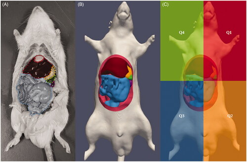
We obtained CT images of a male Sprague Dawley rat using a Siemens sensation 64 (120 kVp, 38 mAs, U95u convolution kernel, voxel size: (0.2 × 0.2 × 0.6 mm)). The DICOM images were imported in the open source 3D slicer software [28–31] in which we delineated various organs and the peritoneal wall. Six relevant organs in the peritoneal cavity were included in the model; the liver, spleen, stomach, intestinal tract, pancreas and kidneys. The resulting organ models were translated by maximally five millimeter to mimic physical conditions during an open HIPEC, where organs, such as the bowel, tend to float in the perfusate, also increasing the distance between organs, dominantly in the ventral direction. Inflow and outflow catheters were designed using Salome-Meca [32]. The resulting model was meshed using the build-in OpenFoam feature snappyHexMesh [27]. The number and size of the elements were limited to the order of ∼10⁴ elements to ensure feasible computational times, a stringent factor in CFD simulations. In Figure 1(A,B), we present a comparison between the abdomen of a rat and our reconstructed model. In Figure 1(C), we show the quadrants used for the optimization by evaluating the variation within and between these quadrants. The division into four quadrants provides an excellent basis for experimental monitoring and validation by placing one thermal probe in each quadrant. Placement of more than four probes inside the small peritoneal volume of a rat is not likely to be feasible.

Figure 1. Comparison between a rat with opened abdomen in panel A and the reconstructed model used in this study in panel B. We delineated the organs visible after opening up the rat. Colors indicate the liver (dark red), intestinal tract (light blue), stomach (yellow), spleen (green) and the left kidney (purple). Panel C shows the four quadrants used for analysis of heterogeneities occurring in the peritoneal cavity during the treatment.

Numerical methods

The software used in this study is able to solve equations relevant for simulating the heat and drug dynamics in the fluid volume inside the peritoneal cavity during HIPEC treatments. The software is based on software developed by OpenFoam [27], providing methods to calculate the dynamics according to the Navier–Stokes equations. More specifically, we augmented the chtMultiRegion solver with equations relevant for our treatment planning software. The solver was based on the PIMPLE algorithm, a combination of the PISO (pressure implicit with splitting of operator) and SIMPLE (semi-implicit method for pressure-linked equations) algorithms. We performed transient simulations for the entire duration of a HIPEC treatment, 30 min in our case. All sources, log-functions and constraints were implemented using the fvOptions format offered by OpenFoam [27]. For a more extensive description of the OpenFoam software, we refer to [27,33]. For a description of the software used in this study, we refer to Löke et al. [26].

Heat module

During a HIPEC treatment, there is a profound heat exchange between the rat and the cooler environment. Several components were considered for the heat exchange module. In summary, we can write the steady state energy budget for the rat by (1) $$\begin{array}{c}{Q}_o+Q_{pw}+Q_M-Q_{ab}-Q_s-Q_t=0\end{array}$$(1) where Q_o, Q_pw, Q_M, Q_ab, Q_s, Q_t are the heat received by the rat via the organs (W), the heat received by the rat via peritoneal wall (W), the metabolic rate (W) and the heat lost via the abdominal opening (W), skin and tail (W), respectively. A graphical description of the entire heat compartment model is given in Figure 2(A). This energy budget corresponds to a detailed volume-wise heat interaction resulting in a precise determination of a continuous heat distribution within the organs and peritoneal cavity. Each contribution listed in Equation (1)(1) $$\begin{array}{c}{Q}_o+Q_{pw}+Q_M-Q_{ab}-Q_s-Q_t=0\end{array}$$(1) corresponds to a significant contribution to the overall heat interactions. The live monitoring of the systemic temperature and the dependence of the various contributions on the systemic temperature results in heat flowing back into the system, resulting in a more accurate determination of the heat distribution. We discuss the contributions in detail below.

Figure 2. Modules used for the treatment planning software. Panel A shows the thermal module and panel B the chemotherapeutic module. All organs and the peritoneal cavity are visualized by separate compartments. The arrows between the organs and peritoneal compartment show the heat exchange in A and chemotherapeutic supply in B. The organ compartments are a heat source, Q_o, for the core temperature, T_a, and a source for the systemic drug concentration via S_v. These sources for systemic conditions translate to the sink terms in the organs itself, both drug and thermally related. Drug sinks are based on Baxter and Jain [39] while the heat sink is modeled after the Pennes bio-heat equation [34]. The contributions Q_o, Q_s, Q_t and Q_pw depend on the core temperature. To ensure realistic values, we monitor the core temperature live during the simulation, ensuring that the heat is not entirely lost from the system. The heat exchange with the environment through the opened abdomen amounts to a significant heat loss from the peritoneal cavity, Q_ab, where environmental conditions are set at a constant 22 °C. The systemic concentration decreases due to elimination from the plasma and interaction with the peripheral concentration compartment. All sources and accompanying constants are given in Tables A1 and A2.

The heated fluid in the peritoneal cavity is bound to heat up the organs as well. The heat build-up in the organs is partly carried away by the blood flowing through the organs. This process is governed by the perfusion term featured in the Pennes bioheat equation [34]. The total heat provided by the organs is the sum of the contribution of all cells in all organs (2) $$\begin{array}{c}{Q}_o={\Sigma }_o{\mathrm{ }\Sigma }_{\mathit{cell}}{q}_{o,\mathit{cell}}, \end{array}$$(2) where the contribution per cell is given by the perfusion term given in the Pennes bioheat equation (3) $$\begin{array}{c}{q}_{o,\mathit{cell}}=w_b{·c}_b·\left(T_a-T_{\mathit{cell}}\right), \end{array}$$(3) where w_b, c_b, T_a, T_cell are the mass flow rate per unit volume of tissue (kg/s/m³), blood specific heat (J/kg/K), arterial temperature (K) and temperature in the cell (K). The contribution of the peritoneal wall, Q_pw, was taken into account in a similar way, but instead of a volume-wise approach, adding contributions from individual cells, we used a surface-wise estimation. The temperature was assumed to be homogeneous over the peritoneal wall and constant over the peritoneal wall thickness (1 mm). The real-time temperature over the peritoneal wall was averaged and combining the thickness, the surface area of the peritoneal wall and a perfusion term comparable to a mixture of muscle and fatty tissues we determined the contribution Q_pw. The third and last positive contribution to the heat budget is the metabolic heat rate, Q_M, which we estimate by assuming that the rat can maintain its core temperature at 32 °C [35], the body temperature of rats under anesthesia. The heat generation is then assumed equal to the heat loss.

Two main pathways are responsible for heat loss from the rat: a direct heat loss from the opened peritoneal cavity and an indirect loss from heating elsewhere from the rat due to heated blood flowing out of the cavity. The opened abdomen causes significant heat loss, which we denote Q_ab. This is the direct heat loss from the peritoneal cavity. The value for Q_ab is the sum of the heat loss through radiation, evaporation and convection, and is given by (4) $$\begin{array}{c}{Q}_{ab}=Q_{ab,\mathit{radiation}}+ Q_{ab,\mathit{evaporation}}+ Q_{ab,\mathit{convection}}, \end{array}$$(4) respectively. We estimate the radiative heat loss by using the Stefan–Boltzmann law [36] (5) $$\begin{array}{c}{Q}_{ab,\mathit{radiation}}={\sigma }_{sb}·ϵ·\left(T^4-T_{\mathit{amb}}^4\right), \end{array}$$(5) where ε, σ_sb and T_amb are the emissivity of the skin (−), the Stefan–Boltzmann constant (J/K) and the ambient temperature (K) (see Table A1 for values). Estimating the evaporative heat loss is more complicated. We estimate the relative humidity to be around 30% in laboratories where rat HIPEC experiments take place. The average flow velocity caused by drafts and/or fume hoods is estimated to be around 0.5 m/s, also the lower bound of measurable airflow. The contribution of evaporation to the energy budget can be calculated using [37] (6) $$\begin{array}{c}{Q}_{ab,\mathit{evaporation}}=h_{\mathit{evaporation}}·g_s \end{array}$$(6) where h_evaporation is the heat of vaporization (J/kg) and g_s is the mass evaporation rate (kg/s/m²). We assume that the fluid motion is negligible such that we consider the problem similar to air flowing over a still pool of water. Using interpolations between the fluid surface and the room conditions, we can estimate the evaporation rate using (7) $$\begin{array}{c}{g}_s=\frac{D·\overline{{Nu}_{m,l}}\mathrm{ }·{\rho }_f}{L}, \end{array}$$(7) where D is the diffusivity of air m²/s, ρ_f is the fractional density of the aerosolized fluid (kg/m³), L is the contact length between the fluid and the air (m) and $\overline{{Nu}_{m,l}}$ is the mass transport Nusselt number (−) given by (8) $$\begin{array}{c}\overline{{Nu}_{m,l}}=0.664·{R{e}_L}^{\frac{1}{2}}·{Sc}^{\frac{1}{3}}, \end{array}$$(8) where Re_L and Sc are the Reynolds number (−) and Schmidt number (−) of the air at the surface of the fluid. We can calculate the Reynolds number by using (9) $$\begin{array}{c}R{e}_L=\frac{u·\mathrm{ }L}{{\nu }_f}, \end{array}$$(9) with flow velocity, u, estimated around 0.5 m/s and viscosity calculated using the mass fraction, fractional density and interpolated film temperature at the surface of the fluid based on room and surface temperatures. The Schmidt number is defined as the ratio of viscosity and diffusivity and can be calculated by (10) $$\begin{array}{c}Sc=\frac{{\nu }_f}{D} \end{array}$$(10)

The convective contribution can be calculated in a similar way [37] (11) $$\begin{array}{c}{Q}_{ab,\mathit{convection}}=\overline{h\mathrm{ }}·\Delta T, \end{array}$$(11) where $\overline{h }$ and ΔT are the average heat transfer coefficient (W/m²/K) and the temperature difference between the surface and the ambient temperature (K). The average heat transfer coefficient can be determined by using (12) $$\begin{array}{c}\overline{h\mathrm{ }}=\frac{N{u\_h,L}_{}·\mathrm{ }{k}_{\mathit{air},22C}}{L}=\frac{0.664·\mathrm{ }R{e}_L^{\frac{1}{2}}\mathrm{ }·{Pr}^{\frac{1}{3}}·{\mathrm{ }k}_{\mathit{air},22C\mathrm{ }}}{L}, \end{array}$$(12) where Pr and k_air,22C are the Prandtl number and the heat conductivity. The total heat loss through the opened abdomen is the sum of all three components, see Equation (4)(4) $$\begin{array}{c}{Q}_{ab}=Q_{ab,\mathit{radiation}}+ Q_{ab,\mathit{evaporation}}+ Q_{ab,\mathit{convection}}, \end{array}$$(4) , and was estimated to be around $\approx 50\frac{W}{m^2}+ 440\frac{W}{m^2}+110\frac{W}{m^2} \sim 660\frac{W}{m^2},$ respectively.

A part of the heat transferred to the blood is lost to the environment, establishing the indirect heat loss from the peritoneal cavity. We take two ways into account in which rats can lose their body heat. First of all, there is significant heat loss to the exterior via the skin (Q_s). We used a separate perfusion term to take this into account similar to Equation (3)(3) $$\begin{array}{c}{q}_{o,\mathit{cell}}=w_b{·c}_b·\left(T_a-T_{\mathit{cell}}\right), \end{array}$$(3) . The second way is via the rat tail (Q_t), used for thermal regulation. At an ambient temperature of 22 °C, the perfusion for the tail vein is minimal. However, if the core temperature increases during HIPEC, the perfusion in the rat tail also starts to increase, resulting in significant heat loss through the tail. We take this into account by replacing the constant w_b with a temperature-dependent mass perfusion term in Equation (3)(3) $$\begin{array}{c}{q}_{o,\mathit{cell}}=w_b{·c}_b·\left(T_a-T_{\mathit{cell}}\right), \end{array}$$(3) . This mass perfusion term is based on experimental data taken from [38]. These data were fitted linearly between 37 °C and 43 °C, yielding (13) $$\begin{array}{c}{w}_b\left(T\right)=180· T-5.58\times {10}^4, \end{array}$$(13) with T (K). The rest of the heat carried away from the organs elevates the core body temperature. The contributions Q_o, Q_s, Q_t and Q_pw depend on the core temperature. To ensure realistic values, we monitor the core temperature throughout the simulation.

Chemotherapy module

The chemotherapy module used in this study has a similar layout. We can write the drug concentration in the systemic compartment, C_sys, as (14) $$\begin{array}{c}\frac{\partial C_{\mathit{sys}}}{\partial t}=S_v-K_e·C_{\mathit{sys}}-K_{12}·C_{\mathit{sys}}+K_{21}·C_{\mathit{per}}, \end{array}$$(14) where S_v, (K_e·C_sys), (K₁₂·C_sys) and (K₂₁·C_per) represent the contribution from the various organs, the elimination from the system, chemotherapy loss to the peripheral compartment, chemotherapy gain from the peripheral compartment. The systemic compartment entails the plasma compartment. The peripheral compartment contains the tissues where the drug interaction is not instantaneous. The peripheral concentration was governed by (15) $$\begin{array}{c}\frac{\partial C_{\mathit{per}}}{\partial t}=K_{12}{·C}_{\mathit{sys}}-K_{21}{·C}_{\mathit{per}}, \end{array}$$(15)

Figure 2(B) shows a graphical representation of the chemotherapy module. The vascular uptake of chemotherapy was determined by using the calculated continuous distribution of chemotherapy.

The chemotherapy is delivered to the organ surface via convection. The chemotherapy diffuses freely into the organs where it is subject to vascular and cellular absorption. Therefore, the total drug sink term S_drug drug can be written as (16) $$\begin{array}{c}{S}_{\mathit{drug}}=S_{\mathit{cell}}+S_v, \end{array}$$(16) where S_cell is the cellular uptake and S_v is the vascular uptake transferred to the central compartment. The sink term is incorporated in the chemotherapy dynamics via (17) $$\begin{array}{c}\frac{\partial \rho C}{\partial t}+ \nabla \left(\rho UC\right)- \nabla \left(D\nabla C\right)+ \rho S_{\mathit{drug}}=0, \end{array}$$(17) where ρ, U, D are the fluid density, fluid velocity and diffusion constant. For more detail, we refer to [26]. We know from experimental in vivo data that the systemic concentration decreases for higher temperatures resulting in a higher cellular uptake [19]. Therefore, we write the cellular uptake as (18) $$\begin{array}{c}{S}_{\mathit{cell}}=\beta · y\left(T\right)·C, \end{array}$$(18) where β a first-order elimination constant (s⁻¹), y(T) is a temperature-dependent enhancement function and C is the drug concentration in the cell. Due to diffusion of the chemotherapy, the chemotherapy concentration C becomes non-zero after some treatment time, and Equation (18)(18) $$\begin{array}{c}{S}_{\mathit{cell}}=\beta · y\left(T\right)·C, \end{array}$$(18) functions as a sink to model cellular uptake. The enhancement function is based on data from [19], which represents the temperature-dependent change in systemic uptake. A first-order approximation was fitted to these data to obtain a continuous function across the hyperthermic temperature range. The function reads: (19) $$\begin{array}{c}y\left(T\right)=0.068 \times T-20.11.\end{array}$$(19)

The vascular uptake is multiplied by this enhancement function. The total vascular uptake then reads [39] (20) $$\begin{array}{c}{S}_v=\left(-\frac{P_c·S}{V}\mathrm{ }\frac{P{e}_v}{e^{P{e}_v}-1}\right)·y^{-1}\left(T\right)· C, \end{array}$$(20) where P_c, S/V and Pe_v are the permeability of the capillary wall (m/s), surface area per unit volume in the tissue (m⁻¹) and the Peclet number (−) reflecting the ratio between convective and diffusive transport in the tissue, respectively. The latter is given by [39] (21) $$\begin{array}{c}P{e}_v=\frac{\left(1-\sigma \right)}{P_c}·L_p·\left(P_v-P_i-c·\left({\pi }_{\mathrm{v}}-{\pi }_i\right)\right),\end{array}$$(21) where σ, L_p, P_v, P_i, c, π_v and π_i are the reflection coefficient (−), hydraulic conductivity (m/Pa/s), arterial pressure (Pa), interstitial pressure (Pa), osmotic reflection coefficient (−), osmotic vascular pressure (Pa) and osmotic interstitial pressure (Pa), respectively. All relevant variables can be found in Table A1.

Boundary conditions

Boundary conditions for the visceral peritoneal surface were chosen to be no-slip for the velocity field and fully transparent for the drug and temperature fields, specifying gradient and value such that the equations are the same on both side of the boundary. The no-slip condition assumes that the fluid has the same velocity at the boundary as the solid boundary itself. In general, this is valid for most in-compressible fluids on macroscopic length scales. The chemotherapy should be able to diffuse freely into the interstitial space of the organs. Therefore, there is a transparent boundary condition for the chemotherapy at the organ boundaries. The interstitial space was modeled to be a fluid porous medium, where the fluid velocity was fixed to zero. We assumed that the temperature was able to penetrate the organs via conduction without influence from boundaries over the organs. Therefore, the thermal boundary condition was also set to act as a transparent condition. At the parietal peritoneal surface, the boundary condition for velocity was chosen to be a no-slip condition as well, for the same reason as before. For the temperature and drug fields, we used the zero-gradient condition, i.e., adiabatic walls at the boundary, assuming no interaction between the internal fields and the boundary field. The parietal peritoneal surface was not modeled volumetric, so no interactions could be modeled there. Instead, the contributions of the parietal peritoneal surface to the systemic chemotherapy concentration and core temperature were included using a surface-wise estimation.

Treatment setup

Catheter orientation and location can have a profound effect on the fluid flow inside the peritoneal cavity. Therefore, we modeled several different catheter setups in the same rat model. The modeled inner catheter lumen diameter was 3 mm. The number of inflow and outflow catheters is very similar to the number of catheters generally used in the clinic. The first setup we consider is a simple setup (#1), where an inflow catheter is placed in the center of the peritoneal cavity, see Figure 3. The inflow is placed toward the back of the peritoneal cavity. The outflow is placed on the surface of the perfusate such that the sagittal distance between the inflow and outflow is maximized. For the second setup, we modeled the inflow between the liver and the stomach and the outflow toward the rectum such that the longitudinal distance is maximized. For the third case, we used the same catheter positions as for the second case, but used both as inflows and we placed the outflow on the surface of the peritoneal perfusate. For the fourth case, we branched the inflow over the frontal axis, while keeping the outflow intact. For the fifth case, we also branched the outflow. The sixth case used all four catheters as inflow catheters and placed the outflow again at the surface of the perfusate. For the cases using one inflow and one outflow, placed between liver and stomach, and two inflows and two outflows, branched over the frontal axis we considered flow alternations as an optimization control. Regions near the outflow tend to be colder than regions near the inflow. During flow alternations, inflow and outflow switch at a certain frequency, possibly improving the homogeneity between inflow and outflow regions. This frequency was chosen to be the equilibration time in the respective non-alternating cases. All setups are visualized in Figure 3 and summarized in Table 1.

Figure 3. Visual representation of the inflow and outflow placement described in Table 1.

The inflow condition was based on a volumetric inflow of 60 ml perfusate per minute, or 1 ml per second which is in the range of flow rates used for rat experiments [40]. This was the same for all cases with varying catheter setups. Consequently, cases featuring two or four inflows had volumetric inflows of 0.5 ml and 0.25 ml per second for four inflows, respectively. We used oxaliplatin as type of chemotherapy in our simulations. The dose was chosen to be 0.16 mol/m³, similar to Lemoine et al., allowing for validation of systemic oxaliplatin concentrations. A clinically relevant inflow temperature of 43 °C was chosen, aiming for a treatment temperature of about 41–42 °C.

To determine the optimal setup, the median temperature and variation in the four quadrants of the peritoneum (Figure 1(C)) was compared between the different catheter setups. For the optimal catheter setup, we consider different flow rates, investigating the effect on the peritoneal surface, both visceral and parietal.

Gravitational effects and laminar flow

To reduce computational effort, we assumed laminar flow and a temperature independent density. To justify this, we determine the influence of natural convection versus forced convection by calculating the Richardson number [41] (22) $$\begin{array}{c}Ri \approx \frac{Gr}{R{e}^2}=\frac{g·\mathrm{ }{\beta }_e·\left(\Delta T\right)·L}{v_{\mathit{max}}^2},\end{array}$$(22) where Gr, Re, g, β_e, ΔT, L and v are the Grashof number, the Reynolds number, gravitational acceleration, thermal expansion coefficient, maximal temperature difference, characteristic length and maximal velocity, respectively. Estimating inflow/maximal velocity around 0.1 m/s, a maximal temperature difference of around 20 °C, between the fluid temperature and the surroundings and using β = 2.07 × 10⁻⁴. We estimate the characteristic length (m) by (23) $$\begin{array}{c}L \sim \frac{V_{\mathit{body}}}{A_{\mathit{body}}} \approx 4\times {10}^{-3}, \end{array}$$(23) we find a Richardson number of 0.016. This is well below 0.1; the limit below which natural convection is negligible. Therefore, we expect that gravity does not have a significant influence on the flow. To evaluate the level of turbulence, we can calculate the Reynolds number: (24) $$\begin{array}{c}R{e}_L=\frac{\rho {·v}_{\mathit{max}}·L}{\mu }, \end{array}$$(24) where ρ and µ are the fluid density and the dynamic viscosity, respectively, and the other symbols as before. We find a Reynolds number of around 600, well below the laminar-turbulent transition occurring around 2500 for a developed flow in a pipe. Therefore, we assume a laminar flow to reduce computation times.

Effective dose

The increased temperatures used during HIPEC enhance the effect of oxaliplatin. To quantify this, we expressed the enhanced cytotoxicity of oxaliplatin as an effective dose by (25) $$\begin{array}{c}Eff. \mathit{Dose}=\mathit{TER}\left(T\right)·C_{ox}\end{array}$$(25) where TER(T) is the temperature-dependent thermal enhancement ratio and C_ox is the oxaliplatin concentration. The thermal enhancement ratio was adapted from an in vitro study published by Urano and Ling [42]. The thermal enhancement ratio per temperature is listed in Table 2. We interpolated the values exponentially using (26) $$\begin{array}{c}TER\left(T\right)=7.085 \times \exp \left(0.256·T\right), \end{array}$$(26) with T (°C).

Table 2. Thermal enhancement ratio of oxaliplatin per temperature, from Urano and Ling [42].

Temperature	Thermal enhancement
37 °C	1
39 °C	1.5
41 °C	2
43 °C	5

Validation

To ensure the validity of our results, we performed two separate tests. The first test was a grid independence study. We used the catheter setup from case # 1 to form three differently sized meshes. The mesh sizes were 47,000, 66,000 and 89,000 hexahedral cells for the low, medium and high refined meshes. We evaluated local and systemic values such as the median oxaliplatin concentration on the surfaces of the organs, median temperature in the four quadrants, the core temperature and the systemic concentration of oxaliplatin. All simulations were performed for a duration of 30 min to ensure that all relevant simulated parameters to have reached an equilibrium.

The results were also compared to experimental studies. The systemic concentration of oxaliplatin was compared to the study performed by Lemoine et al. [43]. In that study, the systemic value of oxaliplatin was measured with a 10 minute time-interval during a 30 min treatment. Measurements were taken at 0, 10, 20 and 30 min. We compare our predicted systemic concentration, determined continuously during the simulation, at these time points with the minimum, maximum and median values reported during those experiments. The calculated core body temperature was compared to a study published by Glehen et al. [44], reporting the average, minimum and maximum core body temperature during a 90 min open-belly treatment. Measurements were taken at 0, 5, 10 and 30 min. To ensure fair comparison, the modeled inflow conditions for the oxaliplatin and the temperature were similar to the inflow conditions used in those studies.

Results

We discuss the results per case as described in Figure 3 and Table 1, with additional flow rate exploration for case # 4. The first case is the standard set-up with one inflow and one outflow. The results using this set-up are discussed in more detail including the validation of systemic parameters and the grid independence study. Then, we show results for cases varying catheter geometry, alternating flow and varying flow rates.

Standard setup

For the standard setup, case #1 in Table 1, inflow and outflow were both in a central location within the peritoneal cavity. The inflow was positioned under the liver with the opening of the catheter placed deep, toward the back of the peritoneal wall. The outflow was positioned at the fluid surface. We performed a grid independence study and validated the standard setup by comparison with values available in the literature.

For the grid independence analysis, we used three meshes, build out of 47,000, 66,000 and 89,000 hexahedral cells. We compared values of relevant parameters as summarized in Table 3. Differences in parameter values between meshes were below 0.5% for the thermal modeling and below 4% for the chemotherapy modeling. Only the systemic concentration can vary over mesh sizes, probably a result of the small variations in surface between mesh sizes and the sensitivity to variations of such a small number. Therefore, the results in this study should be considered grid independent. The mesh with the lowest amount of elements is used in the remainder of this study to reduce computational time.

Table 3. Results of the grid independence analysis.

Parameter	Low refinement	Medium refinement	High refinement
Tmed,pc (°C)	40.42	40.44 (0.05%)	40.47 (0.13%)
Tmed,Q1 (°C)	41.59	41.63 (0.10%)	41.61 (0.05%)
Tmed,Q2 (°C)	40.17	40.14 (0.08%)	40.19 (0.04%)
Tmed,Q3 (°C)	38.41	38.29 (0.31%)	38.24 (0.44%)
Tmed,Q4 (°C)	39.70	39.80 (0.24%)	38.88 (0.45%)
Cmed,pw (µM)	158.80	159.10 (0.19%)	158.85 (0.03%)
Cmed,sp (µM)	87.06	88.56 (1.73%)	90.00 (3.37%)
Cmed,lk (µM)	77.69	78.29 (0.76%)	79.62 (2.48%)
Cmed,rk (µM)	80.95	82.86 (2.37%)	83.57 (3.24%)
Cmed,in (µM)	80.10	80.01 (0.11%)	80.09 (0.01%)
Cmed,st (µM)	100.59	104.45 (3.83%)	102.93 (2.33%)
Cmed,li (µM)	81.74	84.49 (3.37%)	84.00 (2.75%)
Cmed,pa (µM)	103.69	106.29 (2.51%)	107.17 (3.36%)
Tsys (°C)	38.30	38.31 (0.03%)	38.37 (0.17%)
Csys (µmol)	1.61	1.82 (13.11%)	1.70 (5.63%)

We compared T_med,pc, T_med,Q1, T_med,Q2, T_med,Q3, T_med,Q4, T_sys for the thermal module which are the median temperature in the peritoneal cavity, the median temperature in quadrant 1, 2, 3 and 4 and the body core temperature, respectively. For the chemotherapy module, we compared C_sys, C_med,pb, C_med,sp, C_med,lk, C_med,rkb, C_med,in, C_med,st, C_med,li, C_med,pa which are the systemic concentration of oxaliplatin and the median concentrations of oxaliplatin on the surface of the peritoneal wall, spleen, left kidney, right kidney, intestine, stomach, liver and pancreas, respectively. In general variation is limited to a few percent where only relatively large variation is visible for the low systemic concentration of oxaliplatin.

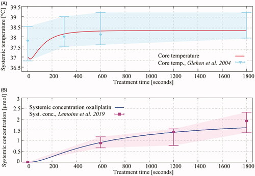
The systemic values were used to compare the model considered in this study to the physical conditions in a rat during a HIPEC treatment. In Figure 4(A,B), we show the comparison between the predicted systemic values with systemic values listed in the literature studies over the entire duration of a HIPEC treatment. The core temperature and systemic concentration predicted by the simulations, red and blue lines, are comparable with experimental data, visualized by the shaded area. The whiskers show the minimum and maximum values and the triangles and squares show the average temperature and systemic concentration of oxaliplatin at that time during the treatment, respectively.

Figure 4. Red (A) and blue (B) lines show the predicted core temperature and the systemic oxaliplatin concentration during a 30 min HIPEC treatment. Experimental data, taken from literature studies shown in the legend are visualized by the shaded area. The whiskers show the minimum and maximum of the measurement in the respective studies. The triangles and squares show the average temperature and systemic concentration of oxaliplatin at that time during the treatment.

Comparing different setups and alternating flow strategies

The first way of optimization considered was varying the location of the inflow and outflow catheter. The second strategy aiming to improve homogeneity was increasing the number of inflow and outflow catheters. The first catheter setup featured a central inflow and a central outflow. The resulting flow velocities are high near the inflow (quadrant 1), but very low near the lower end of the intestine, especially in the third quadrant. This effect resulted in thermal heterogeneities in the third quadrant, clearly visible in Figures 5(B) and 6(A) (case # 1).

Figure 5. 3D representation of the flow velocity (A), temperature distribution (B) and cisplatin concentration (C) around the intestines (light blue), liver (dark red) and stomach (orange) resulting from case # 1. The red and blue catheters represent the inflow and outflow, respectively. The catheter positions are indicative in the 2D plane orthogonal to the depth. A high flow velocity is observed near the inflow next to the stomach. The arrows depict the flow direction. Flow velocities decrease significantly near the rectum of the rat, which result in thermal heterogeneities. The heterogeneities in concentration of chemotherapy are relatively small, although the surface concentrations near the peripheral regions are lower.

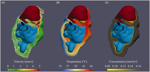
Figure 6. Thermal variation for various catheter setups. Panel A shows the median and interquartile ranges by the vertical lines and the boxes, respectively. The catheter positions are depicted as small dots on top of the graph. For a full representation, we refer to Figure 3. The standard setup, case # 1, shows varying median temperatures between quadrants and large interquartile ranges. The homogeneity and median temperature can be improved by placing the catheters intelligently (case # 2), by addition of catheters (cases # 3, # 4, # 5) or by flow alternation (cases # 6 and # 7). Panels B and C show the thermal patterns in the various quadrants during the treatment. The solid lines show the non-alternating cases (cases # 2 and # 4), while the dashed lines show the thermal patterns of the flow alternations (cases # 6 and # 7). The maximum median treatment temperature is significantly increased in quadrants which are observed to be cold for non-alternating cases.

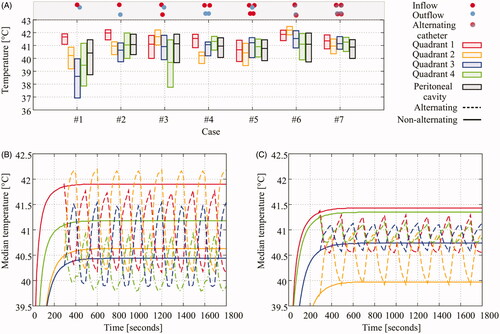
The median temperatures and interquartile variation of all cases are plotted in Figure 6(A). For descriptions of the various cases we refer to Table 1 and Figure 3. Cases 1–5 are based on varying catheter position and the addition of catheters. We see that intelligent placement of catheters, comparison between case # 1 and # 2, improves the homogeneity and the overall median temperature in all quadrants showing significantly smaller interquartile ranges. Addition of catheters further reduces the interquartile range and groups the quadrant median values, albeit slightly. However, the temperature is still heterogeneous for cases # 1–# 4, since one or more median temperatures of a quadrant differs significantly from the other quadrants. Case # 5, using four inflow catheters, shows a low inter-quadrant variation but a relatively large interquartile range. For cases # 2 and # 4, one inflow/outflow and two inflows/outflows, we also considered flow alternations between the inflow and outflow, cases # 6 and # 7, respectively. Flow alternation increases the maximum median temperature in quadrants which were relatively cold without flow alternations. The thermal profiles of the flow alternations are shown in Figure 6(B,C) for cases # 6 and # 7, respectively. The increase and decrease due to the flow alternation are at least two times higher for case # 6 compared to case # 7, a consequence of reducing homogeneity and a higher flow velocity.

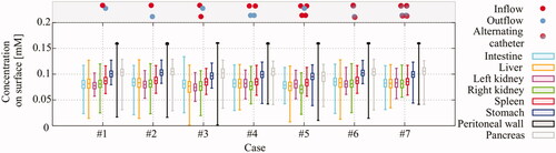
In Figure 7, we show the concentration of oxaliplatin over the surfaces of all organs and over the surface of the peritoneal wall. The variation between cases in minimum, maximum, interquartile ranges and median values is negligible. Case # 4 is chosen as the optimal setup, based on the lowest variation between quadrant interquartile ranges, visible in Figure 6(A). Therefore, we analyzed the influence of flow velocity using setup # 4, using two inflows and two outflows, without flow alternations.

Figure 7. Oxaliplatin concentration variation over surface per organ per case. The boxes show the interquartile ranges and the whiskers show the minimal and maximal concentrations on the respective surfaces during treatment when an equilibrium was achieved. Overall, the variation between cases is negligible.

Flow velocity optimization

Using two inflows and two outflow catheters (case # 4), we investigated a flow rate regime around 1 ml/s. We considered halving and doubling the flow rate. The total amount of oxaliplatin circulated through the peritoneal cavity is kept constant over all flow rates, keeping the total doses uniform over all cases. Therefore, the inflow concentration is halved for a doubled flow rate and the inflow concentration is doubled for halving the flow rate. Increasing the flow rate therefore resulted in lower concentrations of oxaliplatin on the peritoneal surfaces, as observed from Figure 8(A). However, the minimal values were similar for all flow rates. The spread of the oxaliplatin concentration decreased significantly for higher flow rates, visualized by the whiskers in Figure 8(A). The median temperature increased and the spread in the observed temperatures over the surfaces decreased for higher flow rates.

Figure 8. Temperature and oxaliplatin concentration over visceral and parietal peritoneal surfaces for varying volumetric flow rates during a 30 min HIPEC treatment. Total oxaliplatin dose was kept constant for all flow rates resulting in halving the inflow concentration for doubling the flow rate and vice-versa. Whiskers show the minimal and maximal values and the boxes show the interquartile range, with median value visualized by the bar inside the box. Concentration over the surfaces, panel A, changed accordingly. Both the median concentration on the surface and the spread decreased for higher flow rates. The opposite effect is observed for the surface temperatures. Increasing flow rates increased the median temperatures and homogeneity significantly, clearly visible in panel B. The effective dose, a result from the enhanced cytotoxicity due to heat, is a combination of both panels A and B. Using Equation (23)(23) $$\begin{array}{c}L \sim \frac{V_{\mathit{body}}}{A_{\mathit{body}}} \approx 4\times {10}^{-3}, \end{array}$$(23) , we estimated the effective dose on the surface, shown in panel C. For higher flow rates, increased homogeneity is observed without decreasing the effective dose. The effect of varying flow rates to the systemic values is visible in panels D and E. To prevent systemic overheating of the rat, the core temperature should remain below 39 °C.

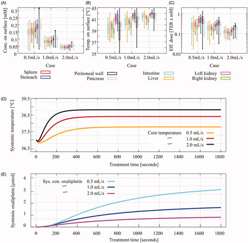
We plotted the effective dose, according to Equation (22)(22) $$\begin{array}{c}Ri \approx \frac{Gr}{R{e}^2}=\frac{g·\mathrm{ }{\beta }_e·\left(\Delta T\right)·L}{v_{\mathit{max}}^2},\end{array}$$(22) , for the various flow rates in Figure 8(C). The gain in homogeneity in Figure 8(A,B) resulted also in a large gain in homogeneity in effective dose. The loss in oxaliplatin on the surface was compensated by an increase in temperature on the surface resulting in a similar effective dose for all flow rates. The variation of flow rates also had an effect on the systemic values, visible in Figure 8(D). Increasing flow rates increased the core temperature by four tenths of a degree while lowering the flow rate lowered the core temperature by six tenths. It is important that the core temperature remains below 39 °C to prevent systemic overheating. This requirement was met for all flow rates. Lowering the flow velocity significantly increased the systemic concentration of oxaliplatin by about 90%. Increasing the flow rate resulted in a lower systemic concentration, about 50% lower.

Discussion

In this study, we presented novel HIPEC treatment planning software based on computational fluid dynamics software, applied to a rat model. The software is able to simulate the flow pattern in the peritoneal cavity and provide a continuous distribution of the chemotherapy concentration and temperature distributions. The software was validated using data from experimental rat HIPEC studies, showing the clinical relevance of the results. We analyzed the effect of different catheter setups, varying in geometry and number of catheters on both the dynamic temperature and drug distribution. The data presented in this study showed that increasing the number of catheters increased the overall homogeneity. Using the optimal setup, setup # 4, we investigated variations in flow rate showing that higher flow rates resulted in more homogeneous and higher effective oxaliplatin doses.

The complexity of the model required the use of various assumptions and estimations. In the thermal module, we estimated the metabolic heat rate based on the assumption that the rat is able to maintain its body temperature at 32 °C while under anesthesia. Hyperthermia could increase the metabolic rate, thus increasing the core temperature and, consequently, increase the peritoneal temperature. Increased perfusion in the organs, also a side effect of hyperthermia, could carry away more heat from the peritoneal tissues, thereby reducing the heat penetration and the peritoneal temperature. Increased perfusion in the skin due to an elevated core temperature was not accounted for. Enhanced skin perfusion would increase the cooling rate of the rat. Furthermore, we assumed a stable environment and stable treatment conditions, which is not necessarily true. Lower ambient temperature would decrease the peritoneal temperature and therefore the treatment temperature. The reduced systemic absorption of oxaliplatin is estimated by interpolating experimental data from [19]. Deviations in the enhancement function, Equation (19)(19) $$\begin{array}{c}y\left(T\right)=0.068 \times T-20.11.\end{array}$$(19) , could increase/decrease the systemic oxaliplatin concentration. The cellular uptake of oxaliplatin was estimated as a first-order elimination constant. Incorporating more detailed interactions, for example adding an oxaliplatin back-flow out of the cell, could increase the interstitial oxaliplatin concentration, possibly resulting in higher systemic oxaliplatin concentrations. However, the outward flux is generally significantly lower than the inward flux, up to around 20–200 times lower [45]. Therefore, the effect is likely to be limited during the short duration of HIPEC. Furthermore, we did not include the physiological characteristics of oxaliplatin in determining the thermal properties of the fluid, like the heat transfer coefficient. In this study, this would have a limited effect because of the small peritoneal volume in rodents. In humans, the peritoneal volume is significantly larger and small perturbations have a larger effect. Therefore, it could be interesting to investigate the effect of the type of chemotherapy on the heat transfer module for human patients. Nevertheless, the qualitative results described in this study, comparing various treatment setups using the same parameters, are not expected to change under these uncertainties. A sensitivity and uncertainty analysis would provide further insight in the influence on the quantitative results.

In varying the catheter setups, we kept the total flow rate constant. The result is a reduced flow velocity for additional inflow catheters in the inflow region. This causes the inflow region to cool more rapidly, possibly translating to a lower temperature in the entire peritoneal cavity. The reduction of flow velocity can also reduce the heating rate of peritoneal surfaces, as demonstrated by Löke et al. [26]. Therefore, the change in homogeneity and median temperature in Figure 6 should be regarded as a lower bound. Increasing flow velocities could increase the additional effect of extra catheters. Two inflow catheters showed the least amount of heterogeneities within each quadrant and four catheters showed the least heterogeneities between quadrants. Our study showed that two inflow catheters would be sufficient and two more does not result in a significant benefit without increasing flow rates. The location of the catheters is however crucial. The optimal location can be found by maximizing the distance between inflow and outflow catheters. We differentiate between outflow catheters placed inside the fluid volume and a outflow catheter at the fluid surface. For catheters placed inside fluid volume, one would have to maximize the distance in the longitudinal direction as in case # 2. In our experience, a challenging aspect of performing HIPEC in small animals like a rat is the blockage of the, relative small, outflow catheter(s) by intraperitoneal tissues. In that respect, a superficial outflow like case # 5 would be more convenient for realizing a continuous unobstructed flow throughout the entire treatment. In that case, four inflow catheters should be used to heat each quadrant separately. If one can ensure a continuous flow with outflow catheters placed inside the cavity, two inflow and two outflow catheters should be preferred (case # 4). The homogeneity as a result of using four catheters is expected to increase when higher flow rates are considered.

We showed in Figure 6 that flow alternations increased the achieved maximum treatment temperature in each quadrant. Experimental use of flow alternation would be challenging. The use of flow alternations would be possible in a closed system, i.e., one perfusate container, driven by a single roller pump switching flow direction over certain intervals. In our study, we assumed instant flow alternations where a delay would be expected in real treatment scenarios. The delay is dependent on the length of the tubes used during the treatment, which would also require rapid heating in the perfusate container to maintain the correct inflow temperature. The alternation frequency is variable. A high frequency, i.e., rapid alternations between inflow and outflow, would result in an insufficient amount of time to cover the entire region near the inflow. Low frequencies, i.e., slow alternations between inflow and outflow, would result in a strong temperature reduction near the outflow catheter. Determining an optimal frequency is important for optimizing the effect of flow alternations. This frequency depends on the total volume of the peritoneal cavity and the volumetric inflow rate at each inflow catheter. In our model, changing flow direction every 4–5 min was optimal but this should be determined in a patient- or model-specific way.

During HIPEC, the surgeon is often manually stirring during open HIPEC (coliseum technique) or hand-assisted laparoscopic HIPEC, or -massages the abdomen during a pure laparoscopic approach to enhance the distribution of chemotherapy and heat. The current software is not able to explicitly model this effect, but it can be accounted for as a reset for the flow patterns. If the stirring or massaging is done without altering the position of the catheters, the same flow pattern will reestablish within a few minutes. Therefore, it is important to change the catheters during massaging and/or stirring and to intercept the flow not too often. The flow should be able to establish a pattern to heat the region after which massaging can take place, for instance every 5–10 min, the optimal frequency for flow alternations.

Choosing an optimal flow rate is a crucial part for an optimal HIPEC treatment. Clinically applied flow rates in patients vary widely (generally between 0.5 and 2 L/min) [4] and there is an overall consensus that higher flow rates increase the heating rate of the peritoneal surface, possibly resulting in a lower visceral temperature [46]. On the other hand, high flow velocities can possibly reduce the coverage of chemotherapy on the peritoneal surface [26]. From the results of the present study, we can conclude that higher flow rates increase the homogeneity of the effective treatment dose. In real-life murine HIPEC experiments, it is difficult to maintain high flow rates. A higher flow rate consequently results in a higher amount of suction near the outflow, increasing the risk of obstructing the outflow catheter. From the results in this study, we can conclude that flow rates should be maximized up to a flow rate where the core temperature is still bearable for the rat, a factor also dependent on the inflow temperature. A flow rate based on the volume of the peritoneal cavity of the patient effectively levels the number of ‘fresh’ volumes a patient receives during a HIPEC treatment. This would reduce the inter-patient variation of the total dose and the chemotherapy concentration in the peritoneal cavity, thereby also increasing the effect of optimizing the thermal distribution.

The outcome parameters predicted in this study, such as the quadrant and systemic temperatures and surface oxaliplatin concentrations, are a result of a delicate balance controlled by Equations (1)–(18). These equations and the physical constants within these equations are not determined in HIPEC-related experiments or for similar applications, and therefore not all equations describe the dynamics down to the finest detail. For example, the equations describing the interaction between the fluid surface and the surrounding air describe the dynamics quite extensively, but in the calculations we assumed that the movement of the fluid was negligible at the surface which is not necessarily true. The assumptions being made on the ambient experimental parameters like the humidity and the local air flow velocity are difficult to validate using the available literature since these values are generally not reported. The heat loss through the tail or the skin is more often investigated and there is relevant literature describing the heat regulation of rats [38]. However, experimental studies investigating the influence of a large heated fluid column on the heat regulation in rats are absent. Additionally, the values of the perfusion terms of the viscera can also have a profound effect on the outcome parameters. We used values based on normothermic conditions. Hyperthermia can have a significant effect on the perfusion in tissues [47] such that we can expect a temperature-dependent perfusion term as in Equation (12)(12) $$\begin{array}{c}\overline{h\mathrm{ }}=\frac{N{u\_h,L}_{}·\mathrm{ }{k}_{\mathit{air},22C}}{L}=\frac{0.664·\mathrm{ }R{e}_L^{\frac{1}{2}}\mathrm{ }·{Pr}^{\frac{1}{3}}·{\mathrm{ }k}_{\mathit{air},22C\mathrm{ }}}{L}, \end{array}$$(12) . Additional experimental studies regarding the perfusion will improve the accuracy of this model, which is also important for extension toward clinical use. To realize the application of treatment planning software for HIPEC, experimental investigation and validation regarding heat regulation in rats as well as in patients, should be prioritized.

In contrast to a compartment model described in the literature to model chemotherapy transport [17,48], we used a continuous model, which also shows the origin of the chemotherapeutic contributions to each compartment. This calculation of a continuous distribution in the organs and the peritoneal cavity is an original and relevant way of determining the dose distribution during and after HIPEC treatments. The calculation of the amount of oxaliplatin absorbed by each organ separately allows logging of the systemic concentration of oxaliplatin. The systemic compartment can then be treated as a regular compartment part of a classical partitioned compartment model involving interactions with the peripheral compartment and obeying the temporal elimination of oxaliplatin from the systemic compartment. The biological interactions between the oxaliplatin and the interstitial space were not fully taken into account. The sink terms in Equations (16)(16) $$\begin{array}{c}{S}_{\mathit{drug}}=S_{\mathit{cell}}+S_v, \end{array}$$(16) and (18)(18) $$\begin{array}{c}{S}_{\mathit{cell}}=\beta · y\left(T\right)·C, \end{array}$$(18) describe the cellular uptake and the vascular uptake, respectively. This does not account for more complex interactions like plasma or protein binding which could possibly affect the amount of oxaliplatin reaching to the systemic compartment and reducing the overall penetration depth. However, for evaluation of heterogeneities inside the peritoneal cavity, this is not an issue since these effects are not likely to change the concentration across the peritoneal surface.

Keeping the abdomen open during HIPEC treatments has advantages and disadvantages. An open abdomen gives the perfusion staff and surgeon the opportunity to intervene during HIPEC and change the position of the catheters. However, heat can easily escape through the opening, affecting the temperature distribution in the peritoneal cavity. Another frequently used technique is keeping the abdomen closed during HIPEC. The abdomen is then closed after the surgery with inflow and outflow catheters placed through separate incisions, similar to a laparoscopic HIPEC. This results in reduced heat loss but there is no possibility to change the position of catheters during treatment. Therefore, flow alternations can be an important tool for optimization of closed HIPEC treatments. Experimental studies are not conclusive on which method is superior in terms of survival and morbidity [49,50]. It is difficult to address the superiority in terms of intra-abdominal homogeneity through experimental studies since the number of measuring points in the abdomen is limited as discussed in section ‘Introduction’. The extension of the model described in this study toward patients provides a unique opportunity to optimize treatment parameters for both open and closed HIPEC treatments and to evaluate the heat and chemotherapy distributions inside the peritoneal cavity. This would provide insight into which treatment method could provide the most homogeneous distributions. The model discussed in this study can be transformed to simulate closed HIPEC treatments by correcting the energy budget, Equation (1)(1) $$\begin{array}{c}{Q}_o+Q_{pw}+Q_M-Q_{ab}-Q_s-Q_t=0\end{array}$$(1) , for the reduced heat loss. Furthermore, during a closed HIPEC, organs have less space to float and are generally closer to each other compared to an open HIPEC treatment, which should be accounted for when generating an anatomical model. The extension of this model toward human patients would also allow to determine the minimum number of thermal probes needed to accurately monitor the temperature distribution in order to guarantee thermal homogeneity.

Expressing the enhanced cytotoxicity of oxaliplatin, or another chemotherapy, as an effective dose clearly demonstrates the importance of both the temperature and the chemotherapy concentration. Our study reflects this point in Figure 8(A,C) where higher flow rates resulted in lower concentrations and higher temperatures on the peritoneal surfaces. If we take the thermal enhancement of oxaliplatin into account, we see that the higher temperatures compensate for the lower oxaliplatin concentration, creating similar median effective doses. A similar behavior can be expected for other chemotherapies or tumor cell types. Although the exact level of thermal enhancement might be different, a positive thermal enhancement exists for chemotherapies used during HIPEC. This aspect of varying thermal enhancement for different tumor types and selected drugs underlines the importance of treatment planning software to support patient and treatment-specific optimization.

The work performed in this study provides a framework for therapy treatment planning software for HIPEC. In the current study, we applied the software to a rat model, and this provides an excellent basis for the development of a treatment setup for preclinical in vivo HIPEC rat experiments. The number of catheters and their placement can be optimized to achieve an optimal homogeneous thermal distribution. Realizing an optimal distribution during preclinical HIPEC experiments, enables to differentiate the effect of the specific relevant parameters on treatment outcome. Development of such a preclinical treatment setup is subject of ongoing research in our group. Catheter position, orientation and the number of catheters are important variables, which are expected to become even more important in human patients because of the larger fluid volume and increased interactions with the surroundings. The modules included can be extended toward human applications. The heat regulation module for human patients should be implemented similar to the one described in Figure 2. Heat interaction regarding the skin, opened abdomen, peritoneal wall and organs were implemented in a surface or volume-specific way and therefore, the same values and equations can be used to describe the heat interaction for humans. The heat module should be extended with human-specific heat regulatory effects; for example, a different metabolic heat rate. In our model, we assumed laminar flow and a temperature independent fluid density to reduce calculation times and increase stability. This was justified for a rat model, but in human patients fluid volumes are larger, so gravitational effects can also become more important. Furthermore, flow velocities are also higher in humans. Therefore, when extending this model toward clinical treatment planning the effect of gravity in larger fluid volumes should be analyzed and evaluated as well as the possible use of a turbulence model.

The level of detail needed and the complex set of equations needed to be solved resulted in long computation times. Despite the simplifications made in this study, modeling was time consuming. We differentiate the process into two parts, the generation of a detailed peritoneal model and the actual computation time. The manual delineation of organs is a time consuming job, but can be resolved by automating the delineation and designing of the anatomical model. Computation times spanned around 72 h using eight out of 16 physical cores on a AMD Ryzen Threadripper 1950X CPU (3.4 GHz, 40MB cache, sTR4). This amount of time is not realistic in clinical applications and more efficient analytical and computational methods will have to be used to make this type of treatment planning software clinically viable. Different implementations of the software and/or efficient parallelization are viable options to realize shorter computation times. The extension toward human application is subject of ongoing research by our group.

Conclusion

The HIPEC treatment planning software developed in this study is able to predict the influence of varying treatment parameters, such as the number and location of catheters, flow alternation and increased flow rates, on the heterogeneity of flow patterns inside the peritoneal cavity of a rat. Adequate placement of inflow and outflow catheters and increasing the number of inflow and outflow catheters increased the median temperature and reduced the overall spread. Increasing the inflow rate increased the level of homogeneity in effective dose significantly. Flow rates are only limited by the core temperature and the technical capability of the setup. Therefore, using multiple inflow catheters and performing flow rate exploration should help in creating optimal treatment conditions for HIPEC. The software provides an excellent basis for HIPEC treatment planning in human applications, which is subject of ongoing research.

Disclosure statement

No potential conflict of interest was reported by the author(s).

Additional information

Funding

This research was funded by the Dutch Cancer Society, UVA grant number 10595.

Appendix A.

Physical constants

Table A1. All physical constants used in this study.

Parameter	Unit	Value	Reference
Qab	W/m^2	600
pa	Pa	101,325
σsb	J/s^1/m^2/K^4	5.67 × 10^−8
Tamb	°C	22
	−	0.98
cb	−	3500	[51]
β	s^–1	7.32 × 10^−4	[52]
Pc	m/s	2.2 × 10^−9	[39]
S/V	m^–1	7 × 10^3	[39]
Ke	h^–1	3.9	[48]
K12	h^–1	2.8	[48]
K21	h^–1	1.1	[48]
Lp	m/Pa/s	2.71 × 10^−12	[39]
σ	−	0.9	[39]
Pv	Pa	2.08 × 10^3	[39]
Pi	Pa	0
c	−	0.91	[39]
πv	Pa	2.67 × 10^3	[39]
πi	Pa	1.33 × 10^3	[39]
Abody	m^2	4.06 × 10^−2
Vblood	L/kg	0.61	[48]
ρblood	kg/m^3	1125
vinflow	m^3/s	1 × 10^−6
Cinflow	mol/m^3	0.16

Table A2. Organ parameters used in this study.

Organ	wb (ml/min/kg)	ρ (kg/m^3)	κ (W/m/°C)	Ch (W/m/°C)
Liver	860	1079	0.52	3540
Pancreas	767	1087	0.51	3164
Intestine	765	1088	0.54	3655
Spleen	1557	1089	0.53	3690
Kidneys	3795	1066	0.53	3763
Stomach	460	1088	0.53	3690
Skin	106	–	–	–
Peritoneal wall^a	33	–	–	–

Values taken from [53].

a Mixture of muscle and fat perfusion terms.

Table 1. Description of cases considered in determining the optimal catheter setup.

Case	Inflows	Outflows	Description	Alternating
# 1	1	1	Inflow positioned between liver and intestine. Outflow positioned at the fluid surface of the peritoneal cavity.	No
# 2	1	1	Inflow positioned between liver and intestine. Outflow positioned at the rectum.	No
# 3	2	1	Inflow positioned between liver and intestine. Inflow positioned at the rectum. Outflow positioned at the fluid surface of the peritoneal cavity.	No
# 4	2	2	Branched inflow such that one inflow is located beneath the liver (Q4) and one beneath the stomach (Q1). Branched outflow positioned such that one outflow is located in Q3 and one in Q2, both near the rectum, see Figure 1.	No
# 5	4	1	Branched inflow such that one inflow is located beneath the liver (Q4) and one beneath the stomach (Q1). Branched inflow positioned such that one inflow is located in Q3 and one in Q2, both near the rectum, see Figure 1. Outflow positioned at the fluid surface of the peritoneal cavity.	No
# 6	1	1	Same as case #2, but with alternating flow between inflow and outflow with frequencies based on equilibration time found for case #2.	Yes
# 7	2	2	Same as case #4, but with alternating flow between inflow and outflow with frequencies based on equilibration time found for case #4.	Yes

The cases are visualized in Figure 3.

References

- Pelz J, Chua T, Esquivel J, et al. Evaluation of best supportive care and systemic chemotherapy as treatment stratified according to the retrospective peritoneal surface disease severity score (PSDSS) for peritoneal carcinomatosis of colorectal origin. BMC Cancer. 2010;10(1):689.
- Thomassen I, van Gestel Y, van Ramshorst B, et al. Peritoneal carcinomatosis of gastric origin: a population-based study on incidence, survival and risk factors. Int J Cancer. 2014;134(3):622–628.
- Testa U, Petrucci E, Pasquini L, et al. Ovarian cancers: genetic abnormalities, tumor heterogeneity and progression, clonal evolution and cancer stem cells. Medicines. 2018;5(1):16.
- Helderman RF, Löke DR, Kok HP, et al. Variation in clinical application of hyperthermic intraperitoneal chemotherapy: a review. Cancers. 2019;11(1):78.
- Verwaal V, van Ruth S, de Bree E, et al. Randomized trial of cytoreduction and hyperthermic intraperitoneal chemotherapy versus systemic chemotherapy and palliative surgery in patients with peritoneal carcinomatosis of colorectal cancer. J Clin Oncol. 2003;21(20):3737–3743.
- Verwaal V, Bruin S, Boot H, et al. 8-Year follow-up of randomized trial: cytoreduction and hyperthermic intraperitoneal chemotherapy versus systemic chemotherapy in patients with peritoneal carcinomatosis of colorectal cancer. Ann Surg Oncol. 2008;15(9):2426–2432.
- van Driel WJ, Koole SN, Sikorska K, et al. Hyperthermic intraperitoneal chemotherapy in ovarian cancer. N Engl J Med. 2018;378(3):230–240.
- Klaver C, Wisselink DD, Punt CJA, et al. Adjuvant hyperthermic intraperitoneal chemotherapy in patients with locally advanced colon cancer (COLOPEC): a multicentre, open-label, randomised trial. Lancet Gastroenterol Hepatol. 2019;4(10):761–770.
- Quenet F, Elias D, Roca L, et al. A unicancer phase III trial of hyperthermic intra-peritoneal chemotherapy (HIPEC) for colorectal peritoneal carcinomatosis (PC): Prodige 7. J Clin Oncol. 2018;36(18_suppl):LBA3503.
- Ceelen W. HIPEC with oxaliplatin for colorectal peritoneal metastasis: the end of the road? Eur J Surg Oncol. 2019;45(3):400–402.
- Rettenmaier MA, Mendivil AA, Gray CM, et al. Intra-abdominal temperature distribution during consolidation hyperthermic intraperitoneal chemotherapy with carboplatin in the treatment of advanced stage ovarian carcinoma. Int J Hyperthermia. 2015;31(4):396–402.
- Elias D, Antoun S, Goharin A, et al. Research on the best chemohyperthermia technique of treatment of peritoneal carcinomatosis after complete resection. Int J Surg Investig. 2000;1(5):431–439.
- Ortega-Deballon P, Facy O, Jambet S, et al. Which method to deliver hyperthermic intraperitoneal chemotherapy with oxaliplatin? An experimental comparison of open and closed techniques. Ann Surg Oncol. 2010;17(7):1957–1963.
- Lévi F, Metzger G, Massari C, et al. Oxaliplatin: pharmacokinetics and chronopharmacological aspects. Clin Pharmacokinet. 2000;38(1):1–21.
- Erlichman C, Soldin S, Thiessen J, et al. Disposition of total and free cisplatin on two consecutive treatment cycles in patients with ovarian cancer. Cancer Chemother Pharmacol. 1987;19(1):75–79.
- den Hartigh J, McVie JG, Van Oort WJ, et al. Pharmacokinetics of mitomycin c in humans. Cancer Res. 1983;43(10):5017–5021.
- Taubert M, Ebert N, Martus P, et al. Using a three-compartment model improves the estimation of iohexol clearance to assess glomerular filtration rate. Sci Rep. 2018;8(1):17723.
- Cotte E, Colomban O, Guitton J, et al. Population pharmacokinetics and pharmacodynamics of cisplatinum during hyperthermic intraperitoneal chemotherapy using a closed abdominal procedure. J Clin Pharmacol. 2011;51(1):9–18.
- Piché N, Leblond FA, Sidéris L, et al. Rationale for heating oxaliplatin for the intraperitoneal treatment of peritoneal carcinomatosis. Ann Surg. 2011;254(1):138–144.
- Szafnicki K, Cournil M, Talabard J-N, et al. Modelling and supervision of intra-peritoneal chemohyperthermia (IPCH). IFAC Proceedings Volumes, Vol. 33, No. 3; 2000. p. 151–154. 4th IFAC Symposium on Modelling and Control in Biomedical Systems; 2000 Mar 30–Apr 1; Karlsburg/Greifswald, Germany; 2000.
- Pang L, Shen L, Zhao Z. Mathematical modelling and analysis of the tumor treatment regimens with pulsed immunotherapy and chemotherapy. Comput Math Methods Med. 2016;2016(2016):6260474.
- Ladhari T, Szafnicki K. Modelling of some aspects of a biomedical process: application to the treatment of digestive cancer (HIPEC). 3 Biotech. 2018;8(4):190.
- Kok HP, Korshuize-van Straten L, Bakker A, et al. Online adaptive hyperthermia treatment planning during locoregional heating to suppress treatment-limiting hot spots. Int J Radiat Oncol Biol Phys. 2017;99(4):1039–1047.
- Kok HP, Kotte ANTJ, Crezee J. Planning, optimisation and evaluation of hyperthermia treatments. Int J Hyperthermia. 2017;33(6):593–607.
- Schooneveldt G, Kok HP, Balidemaj E, et al. Improving hyperthermia treatment planning for the pelvis by accurate fluid modeling. Med Phys. 2016;43(10):5442.
- Löke DR, Helderman RFCPA, Franken NAP, et al. Simulating drug penetration during hyperthermic intraperitoneal chemotherapy. Drug Deliv. 2020. Forthcoming.
- Weller H, Tabor G, Jasak H, et al. A tensorial approach to computational continuum mechanics using object-oriented techniques. Comput Phys. 1998;12(6):620–631.
- Kapur T, Pieper S, Fedorov A, et al. Increasing the impact of medical image computing using community-based open-access hackathons: the NA-MIC and 3D slicer experience. Med Image Anal. 2016;33:176–180.
- Fedorov A, Beichel R, Kalpathy-Cramer J, et al. 3D slicer as an image computing platform for the quantitative imaging network. Magn Reson Imaging. 2012;30(9):1323–1341.
- Kikinis R, Pieper SD, Vosburgh KG. 3D Slicer: a platform for subject-specific image analysis, visualization, and clinical support. New York (NY): Springer; 2014. p. 277–289.
- 3D slicer website; 2020. Available from: https://www.slicer.org/
- Electricité de france, finite element code aster, analysis of structures and thermomechanics for studies and research; 1989–2017. Available from: www.code-aster.org
- Holzmann T. Mathematics, numerics, derivations and OpenFoam(R). 4th ed. Leoben: Holz-Mann CFD; 2017.
- Pennes HH. Analysis of tissue and arterial blood temperatures in the resting human forearm. J Appl Physiol. 1948;1(2):93–122.
- Kiyatkin EA, Brown PL. Brain and body temperature homeostasis during sodium pentobarbital anesthesia with and without body warming in rats. Physiol Behav. 2005;84(4):563–570.
- Colin J, Houdas Y. Experimental determination of coefficient of heat exchanges by convection of human body. J Appl Physiol. 1967;22(1):31–38.
- Lienhard JH IV, Lienhard JH V. A heat transfer textbook. Version 5.00. 5th ed. Cambridge (MA): Phlogiston Press; 2019.
- Raman E, Roberts MF, Vanhuyse VJ. Body temperature control of rat tail blood flow. Am J Physiol. 1983;245(3):R426–R432.
- Baxter LT, Jain RK. Transport of fluid and macromolecules in tumors i. role of interstitial pressure and convection. Microvasc Res. 1989;37(1):77–104.
- Park E, Ahn J, Gwak S, et al. Pharmacologic properties of the carrier solutions for hyperthermic intraperitoneal chemotherapy: comparative analyses between water and lipid carrier solutions in the rat model. Ann Surg Oncol. 2018;25(11):3185–3192.
- Schooneveldt G, Löke DR, Zweije R, et al. Experimental validation of a thermophysical fluid model for use in a hyperthermia treatment planning system. Int J Heat Mass Transf. 2020;152:119495.
- Urano M, Ling C. Thermal enhancement of melphalan and oxaliplatin cytotoxicity in vitro. Int J Hyperthermia. 2002;18(4):307–315.
- Lemoine L, Thijssen E, Carleer R, et al. Body surface area-based versus concentration-based intraperitoneal perioperative chemotherapy in a rat model of colorectal peritoneal surface malignancy: pharmacologic guidance towards standardization. Oncotarget. 2019;10(14):1407–1424.
- Glehen O, Stuart O, Mohamed F, et al. Hyperthermia modifies pharmacokinetics and tissue distribution of intraperitoneal melphalan in a rat model. Cancer Chemother Pharmacol. 2004;54(1):79–84.
- El-Kareh A, Secomb T. A mathematical model for cisplatin cellular pharmacodynamics. Neoplasia. 2003;5(2):161–169.
- Furman M, Picotte R, Wante M, et al. Higher flow rates improve heating during hyperthermic intraperitoneal chemoperfusion. J Surg Oncol. 2014;110(8):970–975.
- Song CW. Effect of local hyperthermia on blood flow and microenvironment: a review. Cancer Res. 1984;44(10):4721–4730.
- Kobuchi S, Katsuyama Y, Ito Y. Mechanism-based pharmacokinetic–pharmacodynamic (PK–PD) modeling and simulation of oxaliplatin for hematological toxicity in rats. Xenobiotica. 2020;50(2):146–153.
- Rodríguez Silva C, Moreno Ruiz F, Bellido Estévez I, et al. Are there intra-operative hemodynamic differences between the coliseum and closed HIPEC techniques in the treatment of peritoneal metastasis? A retrospective cohort study. World J Surg Oncol. 2017;15(1):51.
- Halkia E, Tsochrinis A, Vassiliadou D, et al. Peritoneal carcinomatosis: intraoperative parameters in open (coliseum) versus closed abdomen HIPEC. Int J Surg Oncol. 2015;2015:1–6.
- Lang J, Erdmann B, Seebass M. Impact of nonlinear heat transfer on temperature control in regional hyperthermia. IEEE Trans Biomed Eng. 1999;46(9):1129–1138.
- Steuperaert M, Labate GFD, Debbaut C, et al. Mathematical modeling of intraperitoneal drug delivery: simulation of drug distribution in a single tumor nodule. Drug Deliv. 2017;24(1):491–501.
- Hasgall P, Gennaro FD, Baumgartner C, et al. ITIS database for thermal and electromagnetic parameters of biological tissues. Version 4.0; 2018. https://itis.swiss/