Quantitative prediction of the extent of pelvic tumour ablation by magnetic resonance-guided high intensity focused ultrasound

Abstract

Background

Patient suitability for magnetic resonance-guided high intensity focused ultrasound (MRgHIFU) therapy of pelvic tumors is currently assessed by visual estimation of the proportion of tumor that can be reached by the device’s focus (coverage). Since it is important to assess whether enough energy reaches the tumor to achieve ablation, a methodology for estimating the proportion of the tumor that can be ablated (treatability) was developed. Predicted treatability was compared against clinically achieved thermal ablation.

Methods

MR Dixon sequence images of five patients with recurrent gynecological tumors were acquired during their treatment. Acousto-thermal simulations were performed using k-Wave for three exposure points (the deepest and shallowest reachable focal points within the tumor, identified from tumor coverage analysis, and a point halfway in-between) per patient. Interpolation between the resulting simulated ablated tissue volumes was used to estimate the maximum treatable depth and hence, tumor treatability. Predicted treatability was compared both to predicted tumor coverage and to the clinically treated tumor volume. The intended and simulated volumes and positions of ablated tissues were compared.

Results

Predicted treatability was less than coverage by 52% (range: 31–78%) of the tumor volume. Predicted and clinical treatability differed by 9% (range: 1–25%) of tumor volume. Ablated tissue volume and position varied with beam path length through tissue.

Conclusion

Tumor coverage overestimated patient suitability for MRgHIFU therapy. Employing patient-specific simulations improved treatability assessment. Patient treatability assessment using simulations is feasible.

Keywords:

• High intensity focused ultrasound
• modeling
• pelvis
• treatment prediction
• simulation

1. Introduction

Magnetic resonance-guided high intensity focused ultrasound (MRgHIFU) is a noninvasive therapeutic modality used for several applications, notably the treatment of uterine fibroids [1], metastatic bone pain palliation [2] and essential tremor [3]. It has recently been investigated for thermally ablative treatment of recurrent gynecological tumors (NCT02714621) [4].

Pelvic tumors are challenging to treat with MRgHIFU due to their depth. Moreover, the acoustic beam must avoid acoustically opaque material (e.g., bone, air) and organs-at-risk, while properties of the pre-focal tissues and material that attenuate, reflect, refract and diffract the propagating acoustic beam must be considered. Incorrect selection (or rejection) of patients for MRgHIFU therapy may deprive suitable patients of a therapeutic option, or incorrectly utilize hospital resources by requiring screening sessions for unsuitable patients. The current assessment procedure for patient suitability for MRgHIFU therapy relies on clinical judgment to estimate the proportion of a tumor that can be reached with the HIFU focus (‘tumor coverage’).

Recently, a novel quantitative software-based method of assessing tumor coverage has been developed [5]. However, even where the HIFU focus can be placed in the target tissue, thermal ablation may not be achieved for a number of reasons including removal of heat via blood perfusion [6], and acoustic intensity attenuation with distance [7] which reduces the available focal energy. In addition, the inhomogeneity of patient geometry is known to significantly affect focal pressure, temperature and ablated tissue volume [8]. These factors suggest that assessment of tumor coverage on its own may be inadequate for identifying whether a patient with a relatively deep-seated tumor is suitable for MRgHIFU therapy and that the percentage of tumor that can be thermally ablated (the ‘treatability’) should provide a better assessment. Acousto-thermal simulations have been used previously to estimate the extent of tissue ablation within a patient [8,9] – however, to the authors’ knowledge and probably due to the prohibitive computational costs of these simulations [8–11], work has not progressed toward estimating the treatability of an entire tumor.

In this feasibility study, a novel method for estimating patient treatability from ‘screening images’, in which patients are positioned in a supine oblique treatment position on the MRgHIFU bed, was developed as an extension of a previously developed tumor coverage analysis method [5]. Patient treatment images were used to represent screening images since these show the patient position used clinically. Treatability was predicted using acoustic-thermal simulations. For each patient, the predicted treatability was compared to the tumor coverage (to identify whether the latter could be used as a surrogate measure for treatability) and to the clinically treated tumor volume, to determine the quality of the prediction methodology.

2. Methods

2.1. Overview

Treatability was predicted for five patients using the workflow shown in Figure 1, with details for each step described in the following subsections. The inputs into the workflow were: the patient treatment image datasets, the segmented tumor, bone, body outline, and extracorporeal air, and outputs of tumor coverage analysis estimated using the method described by Lam et al. [5]. Tumor coverage analysis consisted of testing exposure points within the patient for whether they could be reached by the extracorporeal transducer focus, and recording the positions that were reachable. For each reachable exposure point, a standardized volume of tissue (8 mm-diameter by 22 mm-length ellipsoids) around the exposure point was assumed to be thermally ablative in order to generate the tumor coverage volume estimate [5]. The outputs of tumor coverage analysis that were used in this study are the positions of all reachable exposure points expected to provide tumor coverage; the tumor volume covered; and the transducer positions and angulations required to access each reachable exposure point.

Figure 1. Schematic for the methodology used to estimate patient treatability. Inputs include the anatomical patient MR images (representative slices shown here), the three exposure points (magenta), the tumor segment (red), and the covered (i.e., device reachable) tumor volume (yellow overlaid on the tumor segment). The transducer (blue) is positioned and angled such that the geometric focus was placed at reachable exposure points. In step 1, simulation grids are extracted from the larger MR image datasets. In step 2, each grid voxel is assigned acoustic and thermal properties using thresholds. A density image is displayed, with white denoting the densest material (bone) and black denoting the least dense material (oil) in the image. In step 3, an acoustic simulation is performed in order to estimate the acoustic pressure field within the complex distribution of tissues. The pressure field, overlaid on the density map and segmented tumor, shows regions of high (yellow) and low (blue) pressure. In step 4, thermal simulation identifies where tissue ablation should result from acoustic energy absorption and heat transfer. The thermal dose delivered to tissue is calculated. In Step 5, the patient treatability is estimated by examining the positions and volumes of ablated tissues (cyan) for the three exposure points in order to identify the maximum treatable depth, and hence, the treatable tumor volume (output).

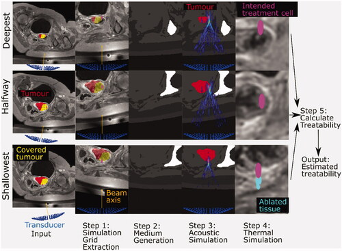
For each patient dataset, three key exposure points were identified from tumor coverage data in order to estimate treatability: the deepest (most anterior in the patient) reachable position within the tumor, the shallowest (most posterior) reachable position within the tumor, and a position within the tumor with its anterior-posterior coordinate halfway between the two. If multiple exposure points were at the same depth, the one closest to the isocentre line (a line going through the positions of the magnetic isocentre of the MRI scanner and transducer home position) was used.

Workflow steps 1–4, inclusive, are the same for each exposure point (deep, shallow, halfway), as described in the caption. Steps 1 and 2 are covered in more detail in Section 2.3, Step 3 in Section 2.4, Step 4 in Section 2.5, and Step 5 in Section 2.6.

2.2. Clinical data acquisition

The data used in this study was obtained from patients who were treated during a clinical trial designed to investigate the treatment of recurrent gynecological tumors with MRgHIFU (NCT02714621) [4,12]. A total of 10 patients with symptomatic recurrent tumors (primary tumors from vulvar, cervical, endometrial and Bartholin gland tissues) that could not be treated with other therapies, or who declined standard treatment, were enrolled in the trial from January 2018 to May 2019. Ethics approval was granted by the NHS Research Ethics Committee (REC: 15/WM/0470), and The Royal Marsden and Institute of Cancer Research Committee for Clinical Research (internal protocol CCR4360) for the use of the clinical trial data in this retrospective study. 6 of the 10 patients were suitable for analysis as their tumors were located within the pelvis, of which only five could be treated with the patient lying in the oblique supine decubitus position used for the development of the tumor coverage methodology. The remaining four patients were unsuitable for analysis as their tumors were located outside the pelvis (one in the knee, three in the groin). The patient data were anonymized before analysis. Patient details are given in Table 1. HIFU therapy was delivered to the patients on a Sonalleve^® V2 MRgHIFU system (Profound Medical, Mississauga, Canada) by a radiographer (SG) and were imaged (Achieva^® 3.0 T, Philips, Netherlands) immediately before, during, and immediately after sonication. Images were acquired using a two-point Dixon sequence [13,14] (field-of-view = 288 × 288 × 133 voxels, voxel resolution = 0.87 × 0.87 × 1.5 mm³, TE1/TE2 = 1.186 (out of phase)/2.372 (in-phase) ms, TR = 3.62 ms, number of echoes =2, flip angle = 10°). Gadolinium contrast enhancement was used. The Dixon sequence produced four datasets for each patient – ‘in-phase’, ‘out-of-phase’, ‘water-only’ and ‘fat-only’ images. The images used in this study were acquired immediately after each treatment session. The angles at which the patients were positioned [5] on the MRgHIFU system during treatment were identified from the imaging datasets using ruler tools in ITK-Snap 3.6.0 software [15] (University of Pennsylvania, USA).

Table 1. Patient details.

Patient	P1	P2	P3	P4	P5
Age (years)	74	59	64	53	72
Weight (kg)	61	61	42	76	57
Treatment angle (degrees)	9	24	6	33	16
Tumor volume (cm^3)	1.2	43.1	13.2	29.1	26.3

2.3. Simulation grid and medium

In order to simulate acoustic propagation in each patient, a 140 × 140 mm wide and 180 mm deep simulation grid containing the transducer was extracted from the 3D MR image dataset in order to reduce the grid size required in the acoustic and thermal simulations and therefore improve computational speed. The grid dimensions were chosen to encompass the transducer and beam dimensions (138 mm widest diameter, 140 mm focal length), with the transducer at the bottom-most portion of the grid aimed directly upwards. Grid axes X, Y and Z are defined as going right-to-left, from the transducer along the beam axis to the geometric focus, and feet-to-head, respectively. As shown in Figure 2, each voxel within the simulation grid was assigned to be a specific tissue or material type. The acoustic, thermal and mechanical properties [16,17] assigned to each tissue or material are listed in Table 2.

Figure 2. The simulation grid (left) extracted from the original patient MR image is segmented into different tissues and materials (right). Physical properties (i.e., density, sound-speed, attenuation coefficient, thermal conductivity, specific heat capacity) were assigned to each voxel based on their tissue/material. For exposure points in which the transducer (blue, left) is situated outside the original patient MR image field-of-view, as in the case in this example (patient P3, halfway exposure point), all voxels outside the original patient MR image field-of-view were assigned the properties of the Sonalleve^® oil (black region, right).

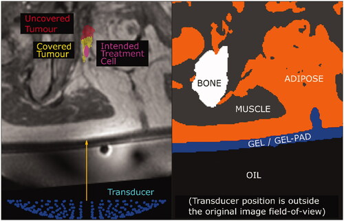
Table 2. Material properties for acoustic and thermal simulation.

	Water (Coupling gel, gel-pad)	Oil	Muscle	Adipose tissue	Bone	Air
Sound speed (m/s)	1517	1380 [58]	1575 [8]	1478 [8]	4080 [8]	1517
Density (kg/m^3)	995.1	840 [58]	1055 [8]	950 [8]	1908 [8]	995.1
Attenuation coefficient ${\alpha }_0$ (dB/MHz^1.1/cm)	0.0022 [8]	0.1	0.6 [8]	0.48 [8]	20 [8]	20
Thermal conductivity (W/m K)	0.60 [17]	0.13 [59]	0.49 [17]	0.21 [17]	0.32 [17]	0.026 [26]
Specific heat capacity (J/kg K)	4178 [17]	1974 [59]	3421 [17]	2348 [17]	1312 [17]	1004 [17]

Sound speed, density and attenuation values for air are explained in the text.

Acoustic pressure attenuation was modeled using the frequency-dependent power-law equation [18,19] (eq (1)(1) $$\alpha ={\alpha }_0{f}^{\gamma }$$(1) ): (1) $$\alpha ={\alpha }_0{f}^{\gamma }$$(1) where $\alpha$ is the attenuation and $f$ is the acoustic frequency. The attenuation coefficient ${\alpha }_0$ and the frequency exponent $\gamma$ are material-dependent properties. Following literature [8], $\gamma$ was defined to be 1.1 for all tissues and materials in this study. Tissue parameters at in-vivo temperatures were used. For oil, properties for temperatures of 25–40 °C were used. Oil attenuation had been previously measured in-house (unpublished data). The sound speed and density of the gel-pad, approximated as water, at 33.5 °C (skin temperature) [20] was obtained from the literature [21,22].

Bone voxels were identified by manual segmentation of MR images using OsiriX Lite [23] 10.0.4 (Pixmeo, Switzerland) and Horos v2.4.0 and v3.0.1 (open-source, https://horosproject.org). The following simple automatic method was used to assign soft tissue or material properties to different voxels: Water-only (W) and fat-only (F) DIXON images were normalized, and then combined to create fat-fraction (FF) images using Equation (2)(2) $$\mathrm{FF}=\frac{F}{W+\mathrm{F}}$$(2) : (2) $$\mathrm{FF}=\frac{F}{W+\mathrm{F}}$$(2)

A threshold-based method was used to assign material properties to voxels [8]. Voxels within the body where $\mathrm{FF}\ge 50\mathrm{\%}$ was assigned the material properties of adipose tissue, and those for which $\mathrm{FF}<50\mathrm{\%}$ were assigned those of muscle. Tumors were modeled as muscle since the sound-speed of tumors (range: 1532 m/s at 22 °C to 1581 m/s at in-vivo temperature) and the attenuation coefficient (range: 0.26–0.70 dB/(MHz^γ cm)) are similar to those of muscle [16].

Voxels outside the body contained air, acoustic coupling gel, gel-pad, or oil. Extracorporeal air was segmented automatically as described in Lam et al. [5]. Non-body, non-air voxels with FF ≥ 0.5 were assigned the properties of the oil, and those with FF < 0.5 the properties of the gel.

The transducer position and angulation required to reach the three key exposure points, determined during tumor coverage analysis [5], ensured that organs-at-risk and acoustic obstructions (i.e., bone and extracorporeal air) were outside the geometric profile of the incident acoustic beam. However, refraction and reflection as the acoustic waves propagate may potentially result in interaction with bone and air. Extracorporeal air in the simulation received special treatment, to avoid the simulation becoming numerically unstable where the interfaces presented sufficiently large impedance mismatches [24], such as between the gel and air (∼10⁴:1), resulting in erroneous results [25]. Therefore, all extracorporeal air voxels were assigned the same sound speed and density as water, but with an arbitrarily high attenuation coefficient of 20 dB/(MHz^1.1cm) to simulate acoustic opacity. In this study, the thermal conductivity of air was taken as 0.0264 W/(m K) [26] and the specific heat capacity was 1003.67 J/(kg K) [17].

Bone voxels were assigned appropriate thermal and attenuation properties. However, the speed of sound in bone is much higher than that in other materials of interest (Table 2), which would require simulations to be performed at a finer time resolution in order to maintain the same numerical accuracy [27]. To avoid this increase in computational requirements, bone voxels were assigned the sound speed of the water, but their density was increased to give the correct acoustic impedance, and hence provide, accurate acoustic reflection at interfaces [7]. In preliminary testing with patient data, this approximation allowed for a six-fold decrease in computation time, with peak acoustic intensity differing by approximately 1%. In addition, because the transducer was positioned and angled such that bone was usually only located outside the acoustic beam, the acoustic energy propagating toward bone, and hence any error due to the unphysical bone sound speed was expected to be negligible.

2.4. Acoustic simulation

The open-source k-wave [28,29] v1.3 package, which uses pseudo-spectral methods to model acoustic wave behavior from coupled first-order partial differential equations, was used. A linear simulation was performed, because the computational resources required for nonlinear simulations were found to be prohibitive even for a high-performance computing cluster. Linear simulations have previously been used to assess how tissue geometry affects kidney HIFU ablation treatments [9]. Because these simulations generally result in less heating at the focus than the nonlinear form [30], using the linear model may represent a worst-case scenario for our purposes.

These simulations produced acoustic pressure fields which, for subsequent thermal modeling, were converted to intensity ($I$) distributions using Equation (3)(3) $$I=\frac{P^2}{2\rho c}$$(3) : (3) $$I=\frac{P^2}{2\rho c}$$(3)

Where P is the zero-to-peak pressure amplitude, $\rho$ is the density, and $c$ is the sound speed.

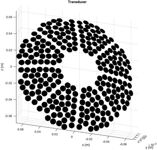
An acoustic pressure source modeled on the geometry of the Sonalleve^® V2 transducer (shown in Figure 3) was used. All simulations were modeled with a source acoustic power of 300 W (the maximum output allowed in the clinical uterine configuration) and at 1.22 MHz. The acoustic simulation ran for the amount of time required for an acoustic wave to travel from one corner of the simulation grid to the opposite corner at the slowest sound speed in the medium (approximately 6700 steps). The spatial resolution was 196 µm (corresponding to 6.2 grid points per wavelength at minimum), and the time resolution was 29 ns (corresponding to a Courant–Friedrichs–Lewy number [27] of 0.25). These settings were chosen because preliminary validation demonstrated that they provided the fastest simulation in which simulated pressures differed by approximately 7% (i.e., no worse than the uncertainty in hydrophone calibration [10] of the validation model’s pressure [31,32]. Simulations were performed on a 20-core (2.6 GHz, 12.8 GB RAM per core) cluster node or a 48-core (2.40 GHz, 8 GB RAM per core) cluster node, depending on which was available.

Figure 3. Transducer used as the source for the acoustic simulations. The 256 6 mm-diameter elements are arranged in a bowl with an outer diameter of 138 mm, 140 mm geometric focal length and an inner hole of 44 mm in diameter.

At each of the three key exposure points (deepest, shallowest or halfway), acoustic pressure fields for a 4 mm-diameter, 10 mm-length treatment cell (that most commonly used for treating these patients, Table 3) were simulated. Clinical treatment cells are generated by electronically steering the ultrasound focus. A 4 mm cell has 8 steered trajectory points on a 2 mm radius circle centered around the exposure point. In preliminary investigations, the simulation at each point required more than 24 h to complete. Computation time was reduced as follows: firstly, an on-axis pressure field, with no phase difference between the transducer elements, was simulated; secondly, to approximate the steered pressure field when sonicating each trajectory point, the on-axis pressure field focus was translated (by 2 mm) to the ‘steered’ focal position. This was done consecutively for all 8 points, based on an assumption that such a small translation through soft tissue would have a negligible effect on the beam profile.

Table 3. Clinical treatment details for each patient.

Patient	P1	P2	P3	P4	P5
Clinically treated tumor volume (ml) [12]	0.08	4.52	0.08	0.00	0.63
Treated volume (% of tumor volume)	7	10	1	0	2
Total energy delivered (kJ) including aborted treatment cells [12]	36.4	23.3	61.7	52.8	97.1
Range of source acoustic powers (W)	140–250	270–300	200–270	220–270	250–290
Number of completed (aborted) treatment cells of diameter:
4 mm	4 (1)	3 (2)	4 (0)	9 (0)	22 (0)
8 mm	5 (0)	4 (6)	11 (0)	5 (1)	1 (0)
Maximum theoretical covered volume from all completed ablations (% of tumor volume)	333	7.4	63.3	15.2	9.8

The clinically treated tumor volumes reported here are those directly from the clinical assessment, and hence their true value may be 30% less. 4 mm and 8 mm-diameter treatment cells have nominal volumes of 84 mm³ and 732 mm³ respectively.

Preliminary simulations through homogeneous media showed that electronically steering the focus 2 mm laterally off-axis reduced the peak intensity to 98.5% that of the on-axis beam. Since the Sonalleve^® system compensates for this by increasing acoustic power [33,34], simulations were all performed at 100% power. For each exposure point in patients, the focal peak pressure was recorded to investigate the variation in focal pressure with a beam path length in tissue (the distance along the beam axis between the exposure point and the skin).

2.5. Thermal simulation

Clinical ablation using treatment cells involves exposing each electronic steering trajectory point for 50 ms, with the switching (HIFU off) time between trajectory points being <10 ms [35]. A regular 4 mm-diameter treatment cell sonication takes 16 s [36]. In order to reduce the risk of burning healthy tissue, a mandatory cooling period for a varying, software-determined period of time [36] (minimum of 30 s) based on estimated energy deposition, is enforced by the control software after each sonication. In this study, the above parameters were replicated in silico. Thermal simulations were conducted using the k-wave package [37] implementation of the Pennes bioheat equation [38] (Equation (4)(4) $$c_p\rho \frac{\partial T}{\partial t}=\nabla \mathrm{ }\cdot \left(K\nabla T\right)+c_b{\omega }_b\left(T-T_b\right)+Q$$(4) ): (4) $$c_p\rho \frac{\partial T}{\partial t}=\nabla \mathrm{ }\cdot \left(K\nabla T\right)+c_b{\omega }_b\left(T-T_b\right)+Q$$(4) (5) $$Q=2{\alpha }_{a}I$$(5)

where $T$ is temperature, $c_p,$ $\rho$ and $K$ are the specific heat capacity, density and thermal conductivity of the medium respectively, ${\omega }_b$ is the blood perfusion rate, $c_b$ is the blood specific heat capacity, $T_b$ is the arterial blood temperature of 37 °C, and $Q$ is the volumetric thermal energy deposited into the medium by absorption of acoustic intensity $I,$ which is calculated at each of the 8 trajectory points from acoustic pressure using Equations (3)(3) $$I=\frac{P^2}{2\rho c}$$(3) and (5)(5) $$Q=2{\alpha }_{a}I$$(5) . The absorption ${\alpha }_a$ is taken to be approximately 75% [39] of the attenuation $\alpha$ (see Equation (1)(1) $$\alpha ={\alpha }_0{f}^{\gamma }$$(1) ). In this study, ${\omega }_b=10$ kg/m³/s [40] and $c_b=3617$ J/(kg K) [17] in all tissue voxels. In order to quantify ablation, the thermal dose was calculated using Equation (6)(6) $$R=\{\begin{array}{c}0.5\mathit{\text{ if T}}\ge 43\mathrm{°C}\\ 0.25\mathit{\text{ if }}37\mathrm{°C}<T<43\mathrm{°C}\\ 0 \mathit{otherwise}\end{array}$$(6) : $$D={\int }_{t=0}^{t_{\mathit{final}}}{R}^{T-43}dt$$(6) $$R=\{\begin{array}{c}0.5\mathit{\text{ if T}}\ge 43\mathrm{°C}\\ 0.25\mathit{\text{ if }}37\mathrm{°C}<T<43\mathrm{°C}\\ 0 \mathit{otherwise}\end{array}$$(6) where $D$ is the thermal dose in units of cumulative equivalent time at 43 °C (CEM43) [41], $T$ is the temperature in degrees Celsius, and the heating and cooling occur between $t=0$ and $t=t_{\mathit{final}}.$ Successful tissue ablation was expected to have occurred at thermal doses ≥240 CEM43 [42].

The simulation was propagated as follows: to represent sonication of a particular trajectory point, the heat source in the bioheat equation, Q, is set to be the volumetric thermal energy deposited at that trajectory point, during a single time step of 50 ms. Then, to represent trajectory switching, Q is set to zero and the simulation is propagated using a single time step of 10 ms. After that, Q is set to be the volumetric thermal energy deposited at another trajectory point, and this cycle is repeated until a total of 16 s (the total sonication duration) has been simulated. Then, to simulate any contribution to thermal dose from the cooling period after treatment, Q is set to zero, and the simulation is propagated with a time step of 0.1 s [43] for a total time of 30 s. All thermal simulations were performed on a 14 CPU-core node (2.60 GHz, 12.8 GB RAM per core).

The ablated tissue (that receiving a thermal dose ≥240 CEM43) was identified for each patient and each exposure point. The positions and volumes of the ablated tissues were used later in estimating treatability. The variation in ablated tissue volume with a beam path length in tissue was explored. The distance between the centroid of the ablated tissue and the intended exposure point, where the treatment cell was centered during tumor coverage analysis, was identified, and its variation with a beam path length in tissue was explored.

2.6. Treatability

2.6.1. Predicted treatability

Patient treatability was defined as the percentage of their tumor predicted to be suitably positioned to receive a cytotoxic thermal dose. Due to the prohibitive computational demands of acoustic-thermal simulation, a simple method was developed for estimating treatability from the simulation results of the three key exposure points (deepest, shallowest, and halfway) for each patient, as described below and depicted in Figure 4.

Figure 4. Schematic diagram illustrating the calculation of the maximum treatable depth. Ablated tissue volume was linearly interpolated as a function of position (depth) between the greater and lesser ablated tissues in order to find the ‘cell-equivalent’ point, where the ablated tissue volume was interpolated to be 84 mm³. The maximum treatable depth was defined to be half a treatment cell length (5 mm for a 4 mm diameter cell) deeper than this point.

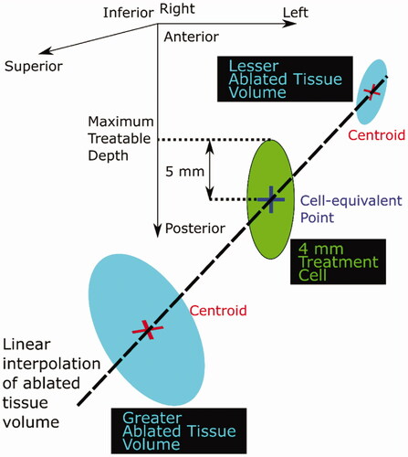
If the ablated tissue volume associated with the shallowest exposure point was less than the expected treatment cell volume (84 mm³ for a 4 mm cell [36], an ellipsoid with the same volume as the ablated tissue volume at the shallowest exposure point was centered at the centroid of that ablated tissue volume, and the maximum depth reached by the ellipsoid was defined as the maximum treatable depth. Otherwise, the ablated tissue volume was linearly interpolated between the two ablated tissue volumes that spanned the expected treatment cell volume (i.e., either the shallowest and the halfway positions, or the deepest and the halfway positions), in order to estimate the position at which the ablated tissue volume would equal the expected treatment cell volume. In the text below and in Figure 4, the position with less than the expected treatment cell volume is denoted as the ‘lesser volume’ position, and that with more is denoted as the ‘greater volume’ position.

The maximum treatable depth (defined in Figure 4) was estimated as shown in the same Figure. If the lesser ablated tissue volume was zero, the lesser volume centroid was estimated by identifying the average distance between the geometric focus and the ablated tissue centroids, and then applying this average distance to the geometric focus associated with the relevant exposure point.

By assuming that all covered tumor volume (identified from prior tumor coverage analysis [5] shallower than the maximum treatable depth is treatable, the percentage of the treatable tumor was calculated. The predicted treatable tumor volume was compared to the covered tumor volume. The dependence on the depth of the tumor beneath the skin (‘tumor-skin distance’), calculated as the distance between the tumor centroid and the skin along a line perpendicular to the MRgHIFU system bed, was also investigated. To identify how deeply the transducer could reach within the tumor, the anterior-posterior distance between the centroids of the ablated tissue associated with the deepest and shallowest exposure points (the ‘ablated tissue separation distance’) was determined for each patient.

2.6.2. Clinical treatability

Patients recruited for the initial feasibility phase of the treatment of recurrent gynecological tumors with MRgHIFU [4] trial were judged clinically as having ≥ 50% tumor coverage. In the treatment trial phase, patients with lower tumor coverage progressed to treatment if clinicians believed sufficient tumor could be sonicated to give patients some clinically relevant benefit, such as pain reduction. Patients were sonicated lying on an acoustic-coupling gel-pad placed over an acoustically transparent membrane above the transducer that was submerged in oil within the treatment bed. Treatment cells were placed using the Sonalleve^® software in order to deliver the treatments summarized in Table 3.

All patients were exposed to 4 mm (16 s sonication duration) and 8 mm (20 s sonication duration) diameter regular treatment cells, with the exception of patient P2 who was treated with 4 mm and 8 mm feedback cells [34,44], in which the heating duration was determined by the Sonalleve^® control software which tried to ensure ablation occurred. For each patient, the number of completed sonications, the range of acoustic powers used per sonication, and the total energy delivered, were recorded. As part of a separate study [12], the clinicians had used the Sonalleve^® control software to manually identify the three maximal orthogonal dimensions of the 240 CEM43 dose contour for each sonication, obtained using proton resonance frequency shift MR thermometry, and multiply them together to obtain the ablated tissue volume associated with the sonication. This resulted in an overestimate of ablated tissue volume per sonication because ablated tissue shape usually resembles an ellipsoid [33,34] rather than the cuboid implied in the above calculation. The overestimation is estimated to be approximately 30%. These ablated tissue volumes had then been summed to obtain the clinically treated tumor volume. No attempt had been made by the clinical team to avoid double-counting ablation of the same tissue by multiple exposures, but they did ensure that all ablated tissue was within the visible tumor boundary. Some exposures had been aborted during heating, probably because the rate of temperature increase had been too slow. Only for patient P2 was the maximum acoustic power of 300 W used for sonication. The maximum volume that could theoretically be ablated by the number of completed treatment cells, as a percentage of the tumor volume, was retrospectively and independently calculated and recorded in Table 3.

3. Results

3.1. Acoustic and thermal simulations

Representative examples of the acoustic pressure fields and tissue ablation generated from simulations are shown in Figures 5 and 6, respectively. Quantitative results are shown in Table 4. As mentioned in Section 2.4, beam path length in tissue is the distance along the beam axis between the centroid of the intended treatment cell (at the transducer geometric focus) and the skin.

Figure 5. Representative cross-sections of simulated acoustic pressure fields (colour bar, only pressures >10% of focal peak pressure are shown) overlaid on the density map (grayscale, lighter means denser, that is, bone is white and oil is black) used for different patients and exposure points. The intended treatment cell (magenta, 4 mm wide, 10 mm long, centered at the geometric focus) is also shown relative to the tumor (red). Each cross-section is the slice in which the peak focal pressure lies.

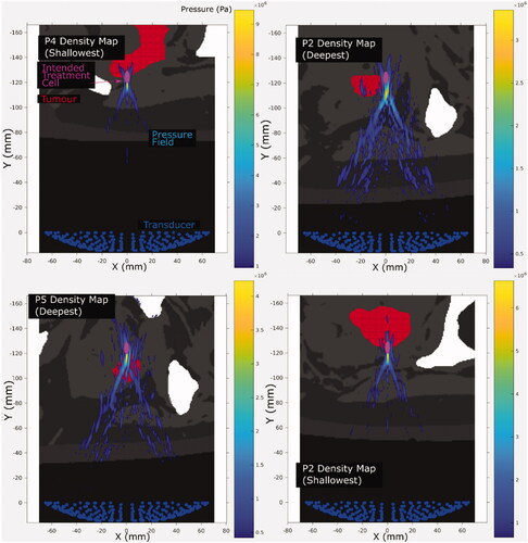
Figure 6. Cross sections of the ablated tissue (cyan), resulting from simulated sonication of the deepest, shallowest and halfway reachable treatment cells (magenta, 4 mm wide and 10 mm long centered at the geometric focus), overlaid on patient anatomy (grayscale in-phase MR image). The image slices are those with the largest ablated cross-sectional area. The ablated tissue volumes’ distances from the geometric focus, in all three dimensions, are quantified in Table 4.

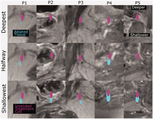
Table 4. Results of acoustic and thermal simulations.

	Patients
Exposure points	P1	P2	P3	P4	P5	Mean ± Standard Deviation
Simulated peak pressure (MPa) ± 10%
Shallowest	6.3	6.6	6.8	9.5	7.9	7.4 ± 1.2
Halfway	6.3	4.2	4.0	7.3	6.0	5.5 ± 1.3
Deepest	6.2	3.4	5.9	4.0	4.2	4.8 ± 1.1
Combined, over all patients	5.9 ± 1.6
Ablated tissue centroid distance from geometric focus (mm) ± 0.2 mm
Shallowest
X	−2.1	0.1	2.0	−0.04	−0.2	−0.4 ± 1.3
Y	8.7	8.0	8.9	5.9	6.6	7.6 ± 1.2
Z	−0.5	−0.2	−0.9	0.04	−0.6	−0.4 ± 0.3
Halfway
X	−2.2	N/A	N/A	−1.4	N/A	−1.8 ± 0.4
Y	8.8	N/A	N/A	9.4	N/A	9.1 ± 0.3
Z	−0.6	N/A	N/A	0.1	N/A	−0.3 ± 0.4
Deepest
X	−2.5	N/A	N/A	N/A	N/A	−2.5 ± 0
Y	8.8	N/A	N/A	N/A	N/A	8.8 ± 0
Z	−0.9	N/A	N/A	N/A	N/A	−1.2 ± 0
Combined, over all patients
X	−0.8 ± 1.4
Y	8.1 ± 1.2
Z	−0.4 ± 0.4
Ablated tissue volume (mm^3) ± 2%
Shallowest	43	52	32	287	130	109 ± 96
Halfway	24	0	0	110	0	27 ± 43
Deepest	7	0	0	0	0	1 ± 3
Combined, over all patients	46 ± 76
Beam path length (mm) in Tissue ± 0.9 mm
Shallowest	61.8	64.5	61.6	45.0	51.6	56.9 ± 7.4
Halfway	63.8	77.4	73.1	67.2	66.6	69.6 ± 4.9
Deepest	64.8	88.7	78.1	87.7	76.5	79.2 ± 8.7
Combined, over all patients	69 ± 12

If the simulated ablated tissue volume is zero, the ablated tissue centroid does not exist, so the distance between ablated tissue centroid position and intended position is denoted as N/A. Positive differences in X, Y and Z between the planned position of the geometric focus and the ablated tissue centroid indicate that the ablated volume is closer to the patient’s left-hand side, the transducer, and the patient’s head, respectively.

Uncertainty in focal peak pressure was estimated, from preliminary validation [32] against a linear analytical model [31], to be under 10%. Uncertainty in the distance between the ablated tissue centroid and the geometric focus was estimated from the simulation grid spatial resolution to be approximately 0.2 mm. Uncertainty in ablated tissue volume was estimated from the discretization of the tumor contours as being approximately 2% of the tumor volume. Uncertainty in tissue path length was estimated from the image resolution to be approximately 0.9 mm.

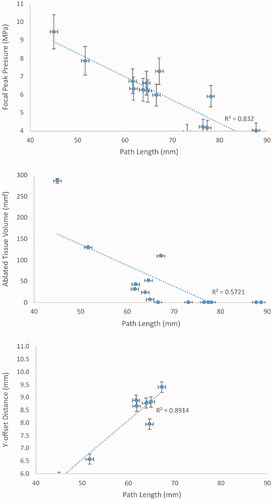
The peak pressure and the ablated tissue positions were, on average, offset from the transducer’s geometric focus by −0.8 ± 1.4 mm in X, 8.1 ± 1.2 mm in Y and −0.4 ± 0.4 mm in Z (i.e., on average, the ablation was displaced slightly toward the patient’s right-hand-side (X), 8 mm toward the transducer (Y), and slightly towards the patient’s feet (Z)). Increasing beam path length in tissue was associated with decreased peak pressure and ablated tissue volume, and increased Y-offset, as shown in Figure 7 with R² numbers.

Figure 7. Focal peak pressure (top), ablated tissue volume (middle) and Y-offset (bottom) dependence on beam path length in tissue. The dotted lines are linear regressions, with the squared correlation coefficients (R²) shown for each regression.

3.2. Treatability

The predicted tumor coverage and tumor treatability are shown visually in Figure 8 with quantitative details being provided in Table 5. Predicted tumor treatability was 52 ± 15% (range: 31–78%) of the tumor volume, less than predicted tumor coverage, and differed from clinically treated tumor volume by 9 ± 9% of the total tumor volume (ranging from the predicted volume being 10% greater than the clinical volume, to being 25% less).

Figure 8. (P1–P5) Cross sections of the predicted treatable volume (cyan), predicted tumor coverage (yellow) and the remaining uncovered and untreatable tumor volume (red) overlaid on patient anatomy (greyscale in-phase MR image). The image slices are those at the position where the interpolated ablated tissue volumes are equal to the expected treatment cell volume (84 mm³). The transducer (138 mm aperture width) is shown for scale.

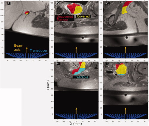
Table 5. Predicted tumor treatable volume compared with clinically treated volume and predicted tumor coverage volume.

Patient	P1	P2	P3	P4	P5
Predicted treatable tumor volume (%)	0	0	0	25	4
Clinically treated tumor volume [12] (%)	7	10	1	0	2
Predicted tumor coverage [5] (%)	47	53	50	56	82
Tumor-skin distance (mm)	64.6	81.5	85.0	69.5	67.5
Ablated tissue separation distance (mm)	2.4	25.9	12.9	37.1	27.3

The tumor-skin distance and the ablated tissue separation distance (both terms defined in Section 2.6.1) are shown for each patient.

For all patients in the study, predicted tumor coverage exceeded predicted treatability. In patients P1, P2, P3 and P5, the difference between predicted treatability and clinically treated tumor volume was relatively low (≤10% of tumor volume). For patients P1, P2 and P3, the maximum treatable depth was shallower than the shallowest exposure point modeled, and resulted in a predicted treatability of 7%, 10% and 1% of the tumor volume less than the clinically observed treated volume respectively. Patients P4 and P5 had treatability predicted to be 25% and 2% of the tumor volume greater than the clinically observed treated volume, respectively. Patients P4 and P5 were the only patients with non-zero predicted treatability. The use of the maximum treatable depth for predicting treatability results in the ‘flat-top’ observed visually for the predicted treatable volumes (cyan) for patients P4 and P5 in Figure 8.

Anatomical differences between patients should be noted. Patient P1’s tumor was surrounded by gluteal subcutaneous fat approximately 65 mm beneath the skin, whereas the other patients’ tumors were bordered by both adipose and aqueous tissue.

Tumor depths and volumes differed between patients. Patient P4’s tumor was relatively shallow (the shallowest exposure point being 45 mm beneath the skin); the shallowest exposure point of the tumors of patients P1, P2 and P3 were at a minimum of 10 mm deeper than for patient P5 (51.6 mm deep for the shallowest exposure point) and 15 mm deeper than for patient P4. For patient P3, the acoustic beam propagates through an asymmetric distribution of adipose and muscle tissue before reaching the tumor (Figure 8).

The total time required to calculate ablated tissue volume per exposure point per patient on the 20-core cluster node was 58 ± 7 h (range: 49–71 h, n = 9), and on the 48-core cluster node, 27 ± 4 h (range: 22–34 h, n = 6).

4. Discussion

The purpose of the methodology developed here for predicting the treatability of pelvic tumors with MRgHIFU therapy was in order to optimize patient assessment to identify those suitable for MRgHIFU treatment. Predicted treatability was compared with both the clinically treated tumor volume and software-based tumor coverage prediction [5]. In current clinical practice, tumor coverage is estimated by the treating clinician when assessing patient suitability for MRgHIFU.

Tumor coverage analysis [5] suggested that 4/5 patients in the clinical trial [4] (all except P1) had tumors for which ≥50% was reachable. Patient P1 progressed to treatment after clinical judgment suggested that enough tumor was reachable to provide a potential medical benefit. As predicted treatable volumes were only 52% (range: 31–78%) of the tumor volume less than the tumor coverage estimate, this suggests that acoustic-thermal simulations may be essential to provide an accurate assessment of patient suitability for deep-seated tumors (64.6–85 mm deep within the body for this study’s patient cohort). Within this small cohort, the lack of a clear relationship between tumor coverage and treatability suggests that treatability cannot be inferred from coverage assessment alone. Hence, clinical assumptions [4] that use tumor coverage as a surrogate for treatability can be inaccurate. It may be possible to improve predictions made from tumor coverage assessment by making adjustments for the relationships between beam path length in tissue and (1) ablated tissue volume, and (2) Y-offset distance (distance along the beam axis between the ablated tissue centroid and the geometric focus), as depicted in Figure 7. Tumor coverage analysis was therefore repeated, using a 4 mm treatment cell-centered 8.1 mm closer to the transducer than the geometric focus. The result was that the predicted treatability was 16 ± 14% of the tumor volume less than the updated tumor coverage estimate. This improvement in tumor coverage assessment suggests that further improvements to the tumor coverage assessment methodology could be worthwhile in order to provide a rapid alternative to computationally intense treatability estimation.

In practice, less than 10% tumor ablation was observed when assessed by MR thermometry in any of the 5 patients. The difference between the predicted treatable tumor volume and the clinically treated tumor volume was 9% of the tumor volume (ranging from 25% of the tumor volume smaller than, to 10% of the tumor volume greater than, the clinically treated volume for different patients). The predicted treatability results in the current study alone suggest that none of the patients should have benefited from treatment. However, patient P1 demonstrated possible tumor necrosis in terms of a tumor region that no longer contrast-enhanced immediately after treatment, an effect that persisted to the end of the 90-day post-treatment monitoring period. There may have been several reasons for this. The clinically observed treated volume may have been inaccurate due to adipose tissue surrounding the tumor, adversely affecting MR thermometry there. Whilst this issue could have affected all patients, no others had radiological findings suggestive of tissue damage – thus, there was no evidence suggesting potential mismeasurement of temperature and no resultant clinical impact. It is also possible that damage to a feeder blood vessel may have resulted in tumor infarction. Furthermore, patient P1 was sonicated using some exposure positions in which the geometric acoustic beam would have intersected air at the edge of the gel pad. In clinical practice, this was avoided by deactivating the transducer elements that would have been obstructed and driving the remaining elements at increased power to compensate. Although this may have resulted in greater defocusing and focal offsets, it may also have allowed a larger volume of patient P1’s tumor to be treated than would have otherwise been possible. However, because the resulting acoustic pressure fields are unpredictable, this capability of the MRgHIFU system was not accounted for when estimating tumor coverage. Hence, the exposure points used for patient P1 in this study may have been unrepresentative. Furthermore, simulations may have underestimated patient treatability in patients P1, P2 and P3 due to a number of other factors, as described below.

Other clinical and methodological hypotheses for the remaining discrepancy between clinical and predicted treatability exist. In this study, blood perfusion was modeled at a constant rate of 10 kg/m³/s [40], which may be greater than recorded blood perfusion in resting muscle (around 0.6 kg/m³/s [17]. Clinically, perfusion varies with temperature history, that is, temperature and duration of heating [45]. Heterogeneous perfusion [46] in different regions of the tumor can significantly affect thermally ablated volumes [47] and hence impact the accuracy of treatability estimation. In pilot simulations, when perfusion was reduced to zero, estimated tumor treatability increased by 18 ± 22% (range: 0–63%, n = 5) of the tumor volume on average. In addition, clinical treatments may have been stopped before completion. For example, since exposures are usually conducted deepest-to-shallowest, it may have been decided to end treatment if a significant proportion of the deeper tumor could not be ablated. Similarly, the maximum available acoustic power of 300 W may not have been used, with the exception of patient P2, due to skin burns and/or subcutaneous fat damage. Reflections and refraction from layers too thin to be observed on the MR image may have also led to differences between predicted and clinical-treated tumor volume.

The discrepancy between predicted treatable volume and that achieved clinically may have arisen from choices in the modeling methodology. A relatively steep angulation of the transducer may be required to reach peripheral regions of the tumor, increasing the beam path length in tissue. Attenuation, refraction and diffraction may therefore be exacerbated, resulting in lower-than-expected heating at the focus during sonication. Treatability estimation could therefore be improved by sampling more exposure points within the tumor to provide more data on which to base estimation, at the cost of increased computational resource requirements. Furthermore, the use of linear simulations in this study meant that focal peak positive pressures and intensities may have been underestimated, for example, patients P1, P2 and P3. For the parameters used in this study, the literature suggests that focal acoustic intensity would increase by approximately 6% due to nonlinear propagation [48], resulting in ∼20% increase in the rate of increase of focal temperature [48]. Since the linearity of the simulation fails to explain the overestimated treatability of patients P4 and P5, it may contribute relatively little to the difference between clinical and predicted treatability.

The clinically observed treated tumor volume may be inaccurate as a result of the methodology used for quantification [12] (i.e., use of the product of maximal orthogonal dimensions rather than the calculation of ellipsoidal volumes, which are 52% less than a cuboid with the same dimensions). This, and ignoring the potential for ablated volumes to be overlapping, may have led to the overestimation of clinically treated tumor volume.

MR thermometry is sensitive to various factors [49]. Thermometry artifacts and inaccuracy may have arisen due to partial volumes of adipose tissue, breathing-induced abdominal motion [50], heat-induced tissue swelling [51,52], and repositioning of the ultrasound transducer between exposures [53]. Depending on the MR thermometry sequence used, thermometry artifacts may under or overestimate temperature in different voxels [54].

The small patient cohort in this study and biological variation between patients means that despite the relatively close quantitative agreement, the relationship between predicted treatability and clinically observed treated tumor volume should not be assumed to be reliably determined. In the literature, small-cohort simulation studies using patient data also show high variance in results [55]. In addition, the clinically treated tumor volumes are relatively small (ranging from 0 to 4.52 ml, representing 0–10% of tumor volumes), meaning that the magnitude of underprediction is capped at 10% of tumor volume. This may result in the prediction methodology appearing to perform better than it would in a larger cohort. Focal peak intensity generally decreased with an increased path length in tissue, for a fixed exposure level of 300 W (Figure 7). This was probably caused by a greater accumulation of the effects of acoustic refraction, reflection and attenuation for deeper tissues. The effect of this was decreased ablated tissue volume with increased beam path length, as shown in the same figure. Observed differences in the ablated tissue volume between patients with similar beam path lengths were probably due to differing patient tissue distributions and geometries in the beam path. This highlights the importance of using patient-specific simulations to predict treatability, and hence, patient suitability for MRgHIFU. Refraction has been shown to have a significant effect on focal pressure [8]. For patient P5, when sonicating the deepest exposure point, the focal pressure with refraction factored into the simulation was approximately 30% less than that without it.

Lastly, this study shows that the deepest 4-mm treatment cells require either greater acoustic power or more time to ablate tissue than the 300 W and 16 s, respectively, currently allowed in the clinical uterine configuration. The clinical implication is that new therapeutic configurations for the Sonalleve^® system may have to be developed for treating tumors with overlying tissue thickness in the range of 45–89 mm.

In the future, treatability estimation could be improved in several ways. The clinical trial data could be retrospectively reanalyzed. Since blood perfusion is an important factor in determining ablated tissue volume, more data may be required on tumor perfusion in response to heat in order to develop a more accurate thermal simulation methodology. The suggestion of improving the treatability estimation method by assessing more points within the tumor would be made more plausible with improved software engineering and a faster simulation methodology, such as hybrid angular spectrum methods [56,57], to allow the assessment of more exposure points and hence increase treatability estimation accuracy without increasing computing time requirements (in this study, 27 ± 4 h). Nevertheless, the treatability estimation methodology introduced in this study outperformed the current clinical assessment method, and the more quantitative tumor coverage method.

5. Conclusions

In this feasibility study, a quantitative method of predicting recurrent gynaecological tumor treatability with MRgHIFU has been developed using treatment image data from a clinical trial and acousto-thermal simulations performed using k-Wave. The predicted treatable tumor volume differed from the clinically treated tumor volume by 9% (ranging from being 10% smaller than the clinical volume to 25% greater). Tumor treatability, predicted from interpolation of simulated ablated tissue volumes, was less than tumor coverage by 52% of the total tumor value (range: 31–78%), suggesting that the current clinical practice of using tumor coverage to assess patient suitability for MRgHIFU therapy should be used with caution. Simple linear relationships for ablated tissue volume and offset distance could be used to improve the current tumor coverage assessment from overestimating treatability by 52 ± 15% of tumor volume to 16 ± 14%. The remaining difference could arise from clinical decisions made during treatment, as well as the relatively simplistic methodology introduced in this feasibility study. Further improvements could be pursued to match simulation results more closely with clinical temperature measurements, to achieve the ultimate goal of quantitative patient assessment for MRgHIFU therapy.

Geolocation information

The study was conducted at the Institute of Cancer Research and the Royal Marsden Hospital, Sutton, Surrey, United Kingdom.

Acknowledgments

The authors would like to thank: Matthew Blackledge, Simon Doran and Matthew Orton from the Institute of Cancer Research (ICR) for their technical support; Bradley Treeby and Elly Martin from University College London (UCL), and Jiří Jaroš from Brno University of Technology, for their support with k-Wave; and Ari Partanen and others from Profound Medical for their support. We are grateful to Philips for their loan of the Sonalleve system to The Royal Marsden Hospital (RMH), and we acknowledge the support of the RMH MRI team, volunteers and patients, the Focused Ultrasound Foundation, CRUK and EPSRC in association with MRC & Department of Health (C1060/A10334, C1060/A16464), the NHS, the NIHR Biomedical Research Centre, the Clinical Research Facility in Imaging, and the Cancer Research Network.

Disclosure statement

The lead author was the recipient of a studentship supported by Philips. This study resulted from research performed as part of a studentship supported by Philips. The views expressed are those of the authors, and not necessarily those of the National Health Service (NHS), the Department of Health, the ICR, the RMH, UCL, Profound Medical, Philips or the NIHR.

Data availability statement

The data that support the findings of this study are not available due to limitations in the ethical review.

Additional information

Funding

The first author (NFDL) produced this work whilst on a studentship supported by Philips. Funding from the NIHR Research for Patient Benefit programme [PB-PG-0815-20001] enabled the acquisition of data for the study.

References

- Sabry M, Al-Hendy A. Medical treatment of uterine leiomyoma. Reprod Sci. 2012;19(4):339–353.
- Hurwitz MD, Ghanouni P, Kanaev SV, et al. Magnetic resonance–guided focused ultrasound for patients with painful bone metastases: phase III trial results. J Natl Cancer Inst. 2014;106(5):dju082.
- Elias WJ, Lipsman N, Ondo WG, et al. A randomized trial of focused ultrasound thalamotomy for essential tremor. N Engl J Med. 2016;375(8):730–739.
- Giles SL, Imseeh G, Rivens I, et al. MR guided high intensity focused ultrasound (MRgHIFU) for treating recurrent gynaecological tumours: a pilot feasibility study. Br J Radiol. 2019;92(1098):20181037.
- Lam NFD, Rivens I, Giles SL, et al. Prediction of pelvic tumour coverage by magnetic resonance-guided high-intensity focused ultrasound (MRgHIFU) from referral imaging. Int J Hyperth. 2020;37(1):1033–1045.
- Kennedy JE. High-intensity focused ultrasound in the treatment of solid tumours. Nat Rev Cancer. 2005;5(4):321–327.
- Hill CR, Bamber JC, Ter Haar GR. Physical principles of medical ultrasound. Hoboken (NJ): John Wiley & Sons; 2004.
- Suomi V, Jaros J, Treeby B, et al. Full modeling of high-intensity focused ultrasound and thermal heating in the kidney using realistic patient models. IEEE Trans Biomed Eng. 2018;65(11):2660–2670.
- Abbas MA, Coussios C-C, Cleveland RO. Patient specific simulation of HIFU kidney tumour ablation. Paper presented at the 2018 40th Annual International Conference of the IEEE Engineering in Medicine and Biology Society (EMBC); 2018 July 17–21; Honolulu, HI.
- Martin E, Jaros J, Treeby B. Experimental validation of k-wave: nonlinear wave propagation in layered, absorbing fluid media. IEEE Trans Ultrason Ferroelectr Freq Control. 2020;67(1):81–91.
- Pinton GF, Dahl J, Rosenzweig S, et al. A heterogeneous nonlinear attenuating full-wave model of ultrasound. IEEE Trans Ultrason Ferroelectr Freq Control. 2009;56(3):474–488.
- Imseeh G, Giles SL, Taylor A, et al. Feasibility of palliating recurrent gynecological tumors with MRGHIFU: comparison of symptom, quality-of-life, and imaging response in intra and extra-pelvic disease. Int J Hyperthermia. 2021;38(1):623–632.
- Dixon WT. Simple proton spectroscopic imaging. Radiology. 1984;153(1):189–194.
- Eggers H, Brendel B, Duijndam A, et al. Dual-echo Dixon imaging with flexible choice of echo times. Magn Reson Med. 2011;65(1):96–107.
- Yushkevich PA, Piven J, Hazlett HC, et al. User-guided 3D active contour segmentation of anatomical structures: significantly improved efficiency and reliability. Neuroimage. 2006;31(3):1116–1128.
- Duck FA. Physical properties of tissue: a comprehensive reference book. Cambridge (MA): Academic Press; 1990.
- Hasgall PA, Di Gennaro F, Baumgartner C, Neufeld E, Lloyd B, Gosselin MC, Payne D, Klingenböck A, Kuster N. IT’IS Database for thermal and electromagnetic parameters of biological tissues, Version 4.0; 2018. DOI:https://doi.org/10.13099/VIP21000-04-0. itis.swiss/database.
- Kelly JF, McGough RJ, Meerschaert MM. Time domain wave equations for lossy media obeying a frequency power law. J Acoust Soc Am. 2008;124(5):2861–2872.
- Szabo TL, Wu J. A model for longitudinal and shear wave propagation in viscoelastic media. J Acoust Soc Am. 2000;107(5):2437–2446.
- Bierman W. The temperature of the skin surface. JAMA. 1936;106(14):1158–1162.
- Bilaniuk N, Wong GSK. Speed of sound in pure water as a function of temperature. J Acoust Soc Am. 1993;93(3):1609–1612.
- U.S. Department of the Interior, Bureau of Reclaimation. Ground water manual. In: Fierro Jr, P, Nyer EK, editors. The water encyclopedia. Washindton (DC): Bureau of Reclaimation; 1977.
- Rosset A, Spadola L, Ratib O. OsiriX: an open-source software for navigating in multidimensional DICOM images. J Digit Imaging. 2004;17(3):205–216.
- Schuster GT. Numerical solutions to the wave equation. In: Seismic inversion. Tulsa (OK): Society of Exploration Geophysicists; 2017. pp. 85–100.
- Robertson JL, Cox BT, Treeby BE. Quantifying numerical errors in the simulation of transcranial ultrasound using pseudospectral methods. Paper presented at the 2014 IEEE International Ultrasonics Symposium 2000–2003; 2014 September 3–6; Chicago, IL.
- Lemmon EW, Jacobsen RT. Viscosity and thermal conductivity equations for nitrogen, oxygen, argon, and air. Int J Thermophys. 2004;25(1):21–69.
- Courant R, Friedrichs K, Lewy H. Über die partiellen {Differenzengleichungen} der mathematischen {Physik}. Math Ann. 1928;100(1):32–74.
- Treeby BE, Cox BT. k-wave: MATLAB toolbox for the simulation and reconstruction of photoacoustic wave fields. J Biomed Opt. 2010;15(2):021314.
- Treeby BE, Jaros J, Rendell AP, et al. Modeling nonlinear ultrasound propagation in heterogeneous media with power law absorption using a k-space pseudospectral method. J Acoust Soc Am. 2012;131(6):4324–4336.
- Filonenko EA, Khokhlova VA. Effect of acoustic nonlinearity on heating of biological tissue by high-intensity focused ultrasound. Acoust Phys. 2001;47(4):468–549.
- O’Neil HT. Theory of focusing radiators. J Acoust Soc Am. 1949;21:516–526.
- Martin E, Ling YT, Treeby BE. Simulating focused ultrasound transducers using discrete sources on regular cartesian grids. IEEE Trans Ultrason Ferroelectr Freq Control. 2016;63(10):1535–1542.
- Köhler MO, Mougenot C, Quesson B, et al. Volumetric HIFU ablation under 3D guidance of rapid MRI thermometry. Med Phys. 2009;36(8):3521–3535.
- Enholm JK, Köhler MO, Quesson B, et al. Improved volumetric MR-HIFU ablation by robust binary feedback control. IEEE Trans Biomed Eng. 2010;57(1):103–113.
- Köhler M, Vaara T, Van Grootel M, et al. MR-only simulation for radiotherapy planning. Amsterdam (The Netherlands): Philips; 2015.
- Philips. Sonalleve MR-HIFU: instructions for use: uterine application and bone application. Vantaa, Finland: Philips; 2012.
- Treeby BE, Wise ES, Cox BT. Nonstandard Fourier pseudospectral time domain (PSTD) schemes for partial differential equations. Commun Comput Phys. 2018;24:623–634.
- Pennes HH. Analysis of tissue and arterial blood temperatures in the resting human forearm. J Appl Physiol. 1948;1(2):93–122.
- Pauly H, Schwan HP. Mechanism of absorption of ultrasound in liver tissue. J Acoust Soc Am. 1971;50(2):692–699.
- Wang M, Zhou Y. Simulation of non-linear acoustic field and thermal pattern of phased-array high-intensity focused ultrasound (HIFU). Int J Hyperthermia. 2016;32(5):569–582.
- Sapareto SA, Dewey WC. Thermal dose determination in cancer therapy. Int J Radiat Oncol Biol Phys. 1984;10(6):787–800.
- Yarmolenko PS, Moon EJ, Landon C, et al. Thresholds for thermal damage to normal tissues: an update. Int J Hyperthermia. 2011;27(4):320–343.
- Dillenseger J-L, Esneault S. Fast FFT-based bioheat transfer equation computation. Comput Biol Med. 2010;40(2):119–123.
- Voogt MJ, Trillaud H, Kim YS, et al. Volumetric feedback ablation of uterine fibroids using magnetic resonance-guided high intensity focused ultrasound therapy. Eur Radiol. 2012;22(2):411–417.
- Vuksanović V, Sheppard LW, Stefanovska A. Nonlinear relationship between level of blood flow and skin temperature for different dynamics of temperature change. Biophys J. 2008;94(10):L78–L80.
- Gillies RJ, Schornack PA, Secomb TW, et al. Causes and effects of heterogeneous perfusion in tumors. Neoplasia. 1999;1(3):197–207.
- Chen L, ter Haar G, Hill CR, et al. Effect of blood perfusion on the ablation of liver parenchyma with high-intensity focused ultrasound. Phys Med Biol. 1993;38(11):1661–1673.
- Soneson JE, Myers MR. Thresholds for nonlinear effects in high- intensity focused ultrasound propagation and tissue heating. IEEE Trans Ultrason Ferroelectr Freq Control. 2010;57(11):2450–2459.
- Rieke V, Pauly KB. MR thermometry. J Magn Reson Imaging. 2008;27(2):376–390.
- Auboiroux V, Petrusca L, Viallon M, et al. Respiratory-gated MRgHIFU in upper abdomen using an MR-compatible in-bore digital camera. Biomed Res Int. 2014;2014(2014):421726.
- McDannold N, Hynynen K, Jolesz F. MRI monitoring of the thermal ablation of tissue: effects of long exposure times. J Magn Reson Imaging. 2001;13(3):421–427.
- Goodman JW. Introduction to Fourier optics. New York (NY): McGraw-Hill; 1996.
- Zhou X, He Q, Zhang A, et al. Temperature measurement error reduction for MRI-guided HIFU treatment. Int J Hyperthermia. 2010;26(4):347–358.
- Rieke V, Butts Pauly K. Echo combination to reduce proton resonance frequency (PRF) thermometry errors from fat. J Magn Reson Imaging. 2008;27(3):673–677.
- Pulkkinen A, Werner B, Martin E, et al. Numerical simulations of clinical focused ultrasound functional neurosurgery. Phys Med Biol. 2014;59(7):1679–1700.
- Vyas U, Christensen D. Ultrasound beam simulations in inhomogeneous tissue geometries using the hybrid angular spectrum method. IEEE Trans Ultrason Ferroelectr Freq Control. 2012;59(6):1093–1100.
- Schwenke M, Strehlow J, Haase S, et al. An integrated model-based software for FUS in moving abdominal organs. Int J Hyperthermia. 2015;31(3):240–250.
- Kreider W, Yuldashev PV, Sapozhnikov OA, et al. Characterization of a multi-element clinical HIFU system using acoustic holography and nonlinear modeling. IEEE Trans Ultrason Ferroelectr Freq Control. 2013;60(8):1683–1698.
- Nadolny Z, Dombek G. Thermal properties of mixtures of mineral oil and natural ester in terms of their application in the transformer. E3S Web Conf. 2017;19:01040.