Feasibility of heating metal implants with alternating magnetic fields (AMF) in scaled up models

Abstract

Aim: Treatment of infected orthopedic implants remains a major medical challenge, involving prolonged antibiotic therapy and revision surgery, and adding a >$1 billion annual burden to the health care system in the US alone. Exposure of metallic implants to alternating magnetic fields (AMF) generates heat that can provide a noninvasive means to target biofilm adhered to the surface. In this study, an AMF system with a solenoid coil was constructed for targeting a metal plate surgically implanted in a sheep model.

Methods: A tissue-mimicking phantom of the sheep leg was developed along with simulation model of phantom and the live sheep leg. This was used evaluate heating with the AMF system and to compare experimental results with numerical simulations. Comparative AMF exposures were performed/simulated in these model for feasibility of design, verification, and validation of simulations.

Results: The system produced magnetic field strengths up to 12mT and achieved plate temperatures of 65–80 °C within 10–14 s. Single and intermittent AMF exposures of a tissue-mimicking phantom agreed with numerical simulations within 5 °C. Similar agreement between experimental measurements and simulations was also observed in the live sheep metal implant model. The simulations also predicted 2–3 mm of tissue damage using a CEM43 thermal dose model for 1-h AMF exposures targeting 65 °C for pulse delays of 2.5 and 5 mins.

Conclusion: This study confirmed that AMF technology can be scaled up to treat implants in a large animal model with the same rates of heating and peak temperatures achieved in prior in vitro studies. Further, numerical simulations provided accurate predictions of the heating produced by AMF on metal implants and surrounding tissues, and can be used to design AMF coils for treating human prosthetic joint implants with more complex geometrical shapes.

Keywords:

• Thermal dose
• alternating magnetic fields
• sheep
• finite element modeling
• system integration

Introduction

Every year, millions of metal orthopedic devices are implanted surgically to treat a range of conditions including skeletal trauma, joint injuries, and osteoarthritis [1]. Amongst the most serious complications associated with metal implants is infection, ranging in incidence from 1 to 3% for prosthetic joints and up to 30% for orthopedic trauma implants [2–4]. These infections are often treated with a 2-stage revision procedure which involves surgical removal of the infected implant, prolonged antibiotic therapy to eradicate the infection [5] and a final surgery to implant a new prosthetic. In addition to a high level of morbidity, revision surgery is associated with a substantial failure rate. Revision total knee arthroplasty develops post-surgical issues 22% of the time due to recurrence of infection which can lead to additional surgeries, amputation, or even death [6–8]. The annual cost to manage prosthetic joint infections (PJI) is approximately $1.1B in the US [9], representing a major health care cost. Furthermore, prosthetic joint replacement is projected to increase by up to 200% in the next decade and is likely to be accompanied by a concomitant increase in infections [10–12]. Beyond the economic cost, the burden to patients of a 2-stage revision procedure is extremely high, resulting in many months of lost productivity and reduced quality of life.

The primary reason infected implants require surgical revision is the formation of biofilm [13,14]. Biofilms are communities of matrix-enclosed bacteria containing extracellular polymeric substances (EPS) secreted by the bacteria, typically 1-mm thick [15–17]. The presence of biofilms impairs the effectiveness of both antibiotic treatment and the innate immune response to infection due to emergence of persister cells. These dormant subpopulations of bacteria with low metabolic rates further reduce the efficacy of antibiotics and advance infection in the host via quorum sensing [18]. In humans, biofilm is found on dental plaque, catheters, and infected metal implants [2]. Due to the characteristics of biofilm, retention of infected metal implants is associated with a risk of infection recurrence after antibiotic therapy.

Alternating magnetic fields (AMF) offer a noninvasive approach for targeting biofilm on metal implants. When conductive materials are exposed to time-varying magnetic fields, electrical currents (referred to as eddy currents) are generated in them. These currents are dissipated as heat in a manner proportional to the magnitude of the induced currents and the electrical conductivity of the material—a process called inductive heating. Since metals have a much higher electrical conductivity than tissue (>10⁶ fold [19–21], metal implants can be heated by induction with negligible direct heating of adjacent tissues. As the AMF frequency is increased, the induced currents increasingly concentrate at the outer surface of the metal through a phenomenon known as the skin effect. At frequencies between 100 and 1000 kHz, the skin depth in metals such as those commonly used in medical implants (titanium, stainless steel, cobalt chrome) is between 0.1 and 1 mm [22]. Furthermore, at these frequencies and magnetic field strengths, the risk of peripheral nerve stimulation in surrounding tissues is very low [23]. An advantage of AMF is that it provides a means to target the surface of metal implants from outside the body, with no interference from overlying tissue or depth limitations within the body [24]. Furthermore, the energy deposited on the implants coincides with the location where biofilm is present. For these reasons, this noninvasive approach to treat implant infection could offer a significant improvement over the current management of PJI.

A growing body of evidence supports the rationale of using heat to target biofilms. Synergy between heat shock at temperatures above 65 °C and antibiotics was observed in vitro for Pseudomonas aeruginosa biofilm with >3 log reduction after 24 h treatment [25]. Staphylococcus aureus and P. aeruginosa biofilms were eradicated along with disruption of the EPS with a 5 min AMF exposure in vitro in a study that also demonstrated that AMF could sensitize biofilm to antibiotics [26]. Studies in mice using small metal bead implants showed less than 1 mm of radial tissue damage a week after AMF exposures of up to 800 W [26]. Induction heating was also used to treat a hip stem in a segmented, non-contact manner using AMF at 360 kHz. This treatment, which reached over 60 °C at the center of the implant (intra-medullary rod), produced temperatures less than 45 °C in the surrounding bone at various distances from the center point. According to calculations based on the CEM43 (cumulative equivalent dose at 43 °C) standard, any thermal damage incurred in surrounding bone tissue is predicted to be reversible [27]. These studies established that heat generated via AMF can eradicate biofilm with high efficiency and rectifiable tissue damage.

An unaddressed challenge is the feasibility of scaling up AMF technology for the treatment of human implants. This presents multiple engineering challenges, including the design of high-power electronics systems to generate magnetic fields with sufficient amplitude, and coils that can be positioned around the body to achieve uniform current density on an implant. Some of these issues were addressed in an earlier body of work investigating the use of induction heating of metal implants for tissue hyperthermia in oncology [28–30]. In these studies, the performance of externally placed coils was investigated in large animals. The heating of implants was limited to 45° C for up to an hour with the goal of heating adjacent tissue through thermal conduction for radio-sensitization. While these studies demonstrated the feasibility of noninvasively heating implants for tissue hyperthermia, they do not provide enough insight into the design of AMF systems for targeting biofilm.

In this study, we investigated the feasibility of constructing an AMF device for the treatment of implant-associated biofilm at the human scale. By using a sheep model with bone-anchored metal plates [31,32], we designed, built, and tested an AMF device, and then validated predictions of numerical simulations against temperature measurements obtained from both phantom and in vivo models. The simulations were employed to address the safety of AMF exposures by assessing thermal dose distributions in tissues under various AMF parameters.

Methods

Geometric models

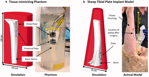
Two geometric models were utilized in this study, shown in Figure 1. The first model was a tissue-mimicking phantom comprised of a cylindrical block of muscle tissue, no blood perfusion, and a sheep tibia mimic with two 2 × 2 cm metal plates (2 mm thick, 316 L stainless steel) attached to it (Figure 1(a)). Five fiberoptic sensors (PRB-G40-2.0M-STM-MRI, Osensa Innovations, Burnaby, Canada) were attached to the front surface and edges of the plate using a high-temperature epoxy (Epotek 353ND, Epoxy Technologies, city, USA). The tibia was constructed using a 3D printer (X-pro, Qidi Tech, Ruian, Zhejiang, China) from a CAD model of a sheep tibia obtained from a CT scan. The tissue-mimicking material was a gellan-gum gel (low-acyl, Modernist Pantry) with electrical and thermal properties similar to muscle at 200 kHz [33]. The primary benefit of the tissue-mimicking phantom was that many thermal sensors could be placed on the metal plate as well as in the surrounding gel for comparison with simulations. Additionally, the tissue-mimicking phantom is a valuable benchtop model for testing AMF coil performance and evaluating heating in different implants prior to in vivo trials. A 3D finite element model of the tissue-mimicking phantom was created to incorporate the locations of fiberoptic sensors to enable comparison between AMF and heating calculations, and experimental measurements.

Figure 1. Geometric models utilized in this study. (a) A tissue-mimicking leg phantom was constructed to mimic a sheep tibia with metal plates affixed to the cortical bone with screws. The leg and plates were embedded in a tissue-mimicking gel phantom and housed in a cylindrical container. Fiber-optic temperature sensors were attached to different faces of the plates as well as in the bone phantom and gel material. (b) A sheep model with the same plates was used to test AMF exposures in vivo, with a corresponding simulation model of the leg incorporating bone, muscle, fascial layers, and skin. Both geometries had corresponding simulation models as shown.

Following sheep experiments were approved by the Institutional Animal Care and Use Committee (IACUC) at University of Utah and conformed to the National Institutes of Health’s PHS Policy on the Humane Care and Use of Laboratory Animals.

Large animal model

The second model consisted of performing terminal surgeries in sheep wherein a simulated fracture fixation plate (same dimensions as in the first model) was secured to the proximal medial aspect of the tibia as described previously [32] (Figure 1(b)). This sheep implant model is a validated surgical model and was used to evaluate the feasibility of heating metal plates with AMF in a large animal.

For surgery, a sheep was first anesthetized (propofol 5-10 mg/kg followed by intubation and isoflurane inhalation 0.5–5.0%) and placed on a circulating water-heated pad. The proximal medial aspect region of the right hind leg was prepped with a betadine skin prep kit. An incision was made at the proximal medial tibia region to expose the flat surface of tibial bone. A simulated fracture fixation plate was then used as a template to drill 4 holes into the bone. Next, a plate with fiberoptic sensors epoxied to the front and side surfaces was fastened to the bone with cortical bone screws (Veterinary Orthopedic Implants catalog #ST 270.00). The fascia was sutured closed and two fiberoptic sensors were secured with sutures such that they resided on top of the fascia above the plate location. Finally, the skin was sutured closed, and a third sensor was secured (with sutures) on top of the skin above the plate location. The sensors were reinforced with surgical tape.

Finite-element simulations

The third model consisted of a 3D simulation model of the sheep leg comprised of sheep bone inside of conical muscle tissue surrounded by air (Figure 1(b)); blood perfusion was included for its comparison with the live animal study. A simulated fracture fixation (same dimensions as first and second models) was placed on the proximal medial aspect of the tibia. To reduce the mesh size and computation time, implant screws were ignored in the 3D rendering, and the leg segment length was truncated without affecting the temperature distribution around the implant. Mesh sizes were tested with a grid independency test by running the simulation for different mesh element sizes and comparing the data.

Details regarding the finite-element models used to simulate AMF exposures in the sheep and phantom model can be found in the Appendix.

AMF coil design and construction

To determine an initial suitable coil design for the plate implant model, the temperature distribution on metal plates exposed to a uniform AMF at 200 kHz in the X, Y and Z directions was calculated (Figure S1). It depicted the heating patterns after 8 s exposure, and the graphs show the mean and standard deviation of the temperatures on the plate. The temperature distribution for a magnetic field in the Y or Z directions produced a more uniform field than the X direction. The Z direction was preferable since slight rotation of the implant about the Z axis would degrade the quality of the heating pattern for a Y field. Therefore, we decided to design a coil to produce a magnetic field primarily in the Z direction. A convenient coil design to achieve this was a simple solenoid, and since it was compatible with placement around the leg of a sheep, this was the coil design selected for this study. Alternative coil designs would be required for more complex implant geometries.

Based on anatomical considerations and initial fit tests with animals, an inner diameter of 14 cm and a length of 25 cm was chosen for the solenoid coil. From prior in vitro and in vivo studies within our group [26,34], we determined that a field strength of approximately 10 − 15 mT was desirable to achieve a rapid heating rate to target temperatures of 65–80 °C in less than 10 s. The relationship between the magnetic field of a solenoid, the coil current, and the number of turns is given by: (1) $$B={\mu }_o\left(\frac{N}{L}\right)I·\text{sin}\omega t$$(1) where, B is the magnetic field [T], u_o is the vacuum permeability constant (4π × 10⁻⁷ N/A²), N is the number of loops, L is the length of the coil [m], I is the RMS current flowing through the coil [A], $\omega$ is the angular frequency [Hz] and t is time [s]. This magnetic field will in turn provide a flux through the cross-section of the implant, producing an EMF as stated by Faraday’s Law of Induction and Lenz’ Law. EMF caused by alternating magnetic fields will produce eddy currents on the implant surface with a skin depth calculated as: (2) $$\delta =\frac{1}{\sqrt{\mathit{\text{πfμσ}}}}$$(2) where, δ is the skin depth [m], f is frequency [Hz], μ is magnetic permeability [H/m] and σ is electrical conductivity of the metal implant [S/m]. These eddy currents within a skin depth cause directed heating of the implant surface due to resistive losses. Therefore, to achieve a specified magnetic field for a required heating rate, either the current through the coil needs to be increased, or the number of loops/unit length. To achieve the high currents required to produce the desired magnetic field, the solenoid was operated as a parallel LC circuit, as this design amplifies the current in the resonant circuit. However, this introduced another design consideration—the inductance of the coil, which is proportional to the number of turns. The resonant frequency of the parallel LC circuit is given by: (3) $$f_o=\frac{1}{2\pi \sqrt{LC}}$$(3) where f_o is the resonant frequency, L is the coil inductance and C is the capacitance of the tank circuit.

A resonant frequency of 200 kHz was chosen to balance achieving skin depth heating and to avoid non-uniform power deposition that arises at higher frequencies. Based on the availability of capacitors capable of high current handling at this frequency, a target inductance of between 30 and 40 µH was suitable for this device. This resulted in a capacitance range between 15 and 20 nF to achieve the desired resonant frequency. Based on preliminary benchtop tests, three 50 nF capacitors (503HC2102K2SM6, Illinois Capacitors, Des Plaines, IL) were selected to be placed in series to obtain a capacitance of 17 nF. These capacitors are conduction cooled and can tolerate up to 1000 V_rms and a maximum root mean square (RMS) current of 60 A at 200 kHz, which was required for this application. For preliminary coil tests, the 20-turn coil was selected with a 1-cm pitch as that provided an inductance of 35 µH. The coil was constructed from 0.63-cm (¼ʺ) OD soft copper tubing (8955K112, McMaster-Carr), to enable water flow through the coil for cooling. For all electrical connections to the coil, 0.63-cm (¼ʺ) clamps were brazed directly onto the tube, and circuit components were fastened by screws onto these clamps. The measured resonant frequency of the combined parallel circuit was 207.8 ± 0.1 kHz.

Impedance matching

Since the electrical impedance of the parallel circuit at the resonant frequency was approximately 15.5 kΩ, a matching circuit was constructed to transform the input impedance to 50 Ω for maximum power transfer. The matching circuit required special components due to the high currents in the circuit which includes a series inductor and parallel capacitor. The series inductor was constructed from two, 10.16-cm (4ʺ) diameter stacked iron-powder cores (T400A-2, Amidon Corporation, Costa Mesa, CA). A 16-AWG magnet wire was hand-wound for 90 turns to achieve an inductance of 640 µH at 200 kHz. The large toroids were necessary to prevent saturation of the core at high power. The parallel capacitor was a variable vacuum capacitor (CMV1-4000-0005, Jennings Technology, San Jose, CA, USA) with a range of 25 − 4000 pF, and a maximum voltage rating of 5000 V. The capacitance was adjusted to achieve fine tuning of the overall circuit impedance to 50 Ω, resulting in 945 pF. A 1.5-m (5 ft) length of wire (10 AWG) was installed between the matching circuit and tank circuit to enable the solenoid to be mounted to the articulating arm for placement over a sheep leg during experiments. The input impedance of the circuit and resonant frequency after matching was 40 Ω and 0˚ phase at 207.8 kHz, respectively.

AMF driving system

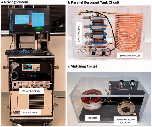
The AMF driving system was comprised of a signal generator (SDS1032X, SIGLENT Technologies, Solon, OH), RF amplifier (1000S04, Electronics and Innovations, Ltd., Rochester, NY), personal computer, and flow system for water cooling (Figure 2). The amplifier delivers up to 1000 W of RF power between 100 and 400 kHz and was controlled by the input signal produced by the signal generator. Ports were available on the amplifier to measure forward voltage and current. The system had a water chiller (MCS, Lytron Inc, Woburn, MA, USA) capable of circulating 5 L/min through the coils and capacitors to remove thermal losses during operation. An articulating arm (VESA Mount TV Arm, VIVO) extended from the driving system setup to hold the solenoid coil at a fixed angle and orientation over the sheep leg. Custom-developed Python software was used to specify the duration, amplitude, and frequency of single or intermittent AMF exposures.

Figure 2. (a) A driving system was developed to power the AMF coils. The system was mobile and had an articulating arm to hold the AMF coil at a desired orientation around the sheep. (b) The solenoid coil is shown with the corresponding capacitors used to form a parallel tank circuit. Both the capacitors and coil were cooled with the water circuit. (c) An impedance matching circuit comprised of a series inductor and parallel capacitor were placed in between the amplifier and the tank circuit to enable efficient power transfer to the coil.

System design and characterization

Power output characterization

Both the net delivered RF power and AC current in the coil were measured with an analog power meter (4410 A, Bird Electronics, Solon, OH, USA) and a Rogowski current probe (TRCP3000, Tektronix, Beaverton, OR, USA), respectively. These parameters were measured as a function of output power by manually increasing the signal input into the amplifier with a function generator (SDS1032X, SIGLENT Technologies, Solon, OH, USA). The input was increased until either the reflected power rose to >30% of forward power or the amplifier went to ‘current overdrive’ (indicating that current delivering capacity had peaked). Achieving more than 30% reflected power before reaching the limit of the amplifier suggested shortcomings of components like saturation of the core for the matching inductor or inability of load or matching capacitor to handle high AC current.

Magnetic field mapping

The magnetic field inside the solenoid coil was mapped in the radial and axial directions using the 2D HF Magnetic field probe (AMF Life Systems, Auburn Hills, MI). The probe was placed in the center of the coil and moved axially upwards from the center in increments of 1 cm to record field strength along its central axis. At each axial measurement point, the radial field was also measured at every 1 cm from the center point along the radius to the inner surface of the coil. These measurements provided a 2D map covering half of axial plane through the center inside the coil and based on the solenoid coil construction, the magnetic field is symmetrical. Based on the symmetry of magnetic field in a solenoid, the field in the other half of the coil was confirmed.

Cooling efficiency

To achieve adequate cooling of the capacitors (surface temperature <45 °C during operation), they were sandwiched between aluminum heatsinks (120959, Wakefield-Vette, Pelham, NH, USA) with 1.5-mm thick silicone thermal pads (7 × 5 cm, Thermal Pad, Aikenuo New Materials, Liaoning, China). The assembly was held together with four threaded rods and tightened with locknuts at each end. The heatsinks along with the copper coil were water cooled in series using a water chiller (5 L/min, MCS, Lytron Inc, Woburn, MA, USA). The efficiency of the cooling system was measured with fiberoptic temperature probes (PRB-G40-2.0M-STM-MRI, Osensa Innovations, Burnaby, Canada). The probes were attached with thermal paste (Type 120, Wakefield-Vette, Inc, Pelham, NH, USA) to conductive surfaces of the following components: load and matching capacitors, iron core for matching inductor, the top and bottom end of the coil, and on the insulation of connecting wires from the matching circuit to the tank circuit.

Tissue-mimicking phantom experiments

Single exposure AMF heating

Experiments were performed in triplicate for single AMF exposure with the phantom centered in the coil (Figure 3) at room temperature (23 °C). AMF pulses with a field strength of ∼12 mT at the center of the coil were delivered to the phantom for durations of 3, 5, 8, 10, 12, and 14 s. The heating rate, cooldown, and temperature rise were determined at various anatomical locations and on the implant plates using fiberoptic sensors for 300 s. The sensors were placed at the center and edge of implant plates to map the temperature distribution. In addition, one sensor was placed ∼2-mm in front of the distal plate and another was placed inside the bone, ∼2-mm behind the proximal plate to measure heat dissipation in tissue with time. Sensor data was recorded using the Osensa System (OSENSA Innovations Corp, BC, Canada). The implants were allowed to cool down close to room temperature before the following exposure.

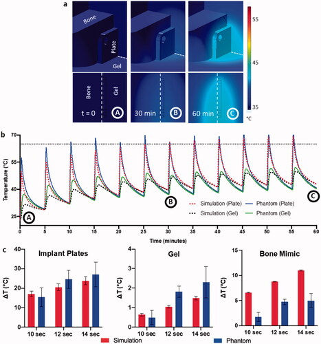
Figure 3. Validation of numerical simulations with phantom data. (a) Volumetric temperature distribution around the implant plate at different timepoints with the dotted red lines showing the cutout location from the volume. (b) Overlaying comparison between simulated and recorded phantom heating curves for a multiple pulse AMF sequence with 14 s exposure with 300 s delay. The points A, B, and C to the time points in a. (c) Correlation between ΔT achieved in simulations and phantom heating for different exposure times on both implant plates, gel, and bone mimic (left to right respectively).

Intermittent AMF heating

An intermittent AMF heating protocol was also executed for the phantom. It included 12 AMF pulses of 10, 12, and 14 s duration and a fixed delay of 300 s between each exposure to allow for cooldown to initial temperature. The temperature data was collected with sensors in the same manner as mentioned above. Heating-cooling cycling continued for 60 min. Mean and standard deviation of ΔT were calculated for all 12 pulses from each fixed heating cycle of AMF exposure to quantify heating variability. All heating experiments were done with 3 replicates. In all cases, phantom initial temperature varied between 23° and 27 °C because of extended cooldown time to reach room temperature for the entire phantom.

Comparison with simulations

Using the tissue-mimicking phantom simulation model (Figure 1), single and intermittent AMF exposures were performed in COMSOL at max. power of AMF system, producing a peak coil current of 120 A and maximum magnetic field of 12 mT at 207.8 kHz. These results were compared with experimental data from phantom heating for maximum power AMF exposures of 10–14 s and cooldown of 300 s. Temperature curves for the center of implant plates and gel sensors were compared with simulation data as well as maximum ΔT values for each AMF exposure duration.

Sheep leg experiments

Single exposure AMF heating

Experiments were repeated for single AMF exposures with the in vivo sheep leg model in triplicate (Figure 4). Before the test, the sheep’s hind leg was inserted into the cavity of the AMF coil and held in place with a stand. Due to increasing leg girth at the abdomen limiting the insertion of the leg, the implant plates were located at the solenoid’s 4th turn from bottom (∼10 mT). AMF exposures with durations of 3, 5, 8, 10, 12, and 14 s were delivered to the sheep leg in the coil. These tests were performed at a field strength of ∼12 mT at the center of the coil and determined the rate of heating, cooldown, and temperature rise at various anatomical locations and the implant plate using fiberoptic sensors for 300 s. Due to limited flat surface area of the upper tibia during the sheep test, only a single (2 × 2 cm) plate was used. Sensor placement (described above) helped measure heat dissipation in different tissue layers with time.

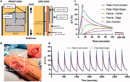
Figure 4. Experimental model for temperature measurement studies in sheep model. (a) Graphical depiction in front and side view of sheep leg for temperature sensor placement. (b) Pictures from surgery with placement of implant plate and sensors going through the hoof and a view after suturing. Temperature readings from all 5 sensors during (c) single 10 s AMF exposure and (d) temperature readings from plate sensors for multiple pulse 10 s AMF exposure with a 325 s delay.

Intermittent AMF heating

An intermittent AMF heating protocol was also executed in sheep. It included 12 pulses, with an AMF exposure duration of only 10 s and a fixed delay of 300 s between each exposure to allow for cooldown to within 5 °C of the initial temperature. The temperature data was collected with sensors in the same manner as mentioned above. Heating-cooling cycling continued for 60 min. Mean and standard deviation of ΔT were calculated for all 12 pulses from each fixed heating cycle of AMF exposure to quantify heating variability. All heating experiments were done with 3 biological replicates during our three sheep tests. Initial temperature for all replicates in sheep varied between 30° and 34 °C with external heating of the leg by using heat pads to maintain initial temperature.

Comparison with simulations

Using the sheep leg simulation model (Figure 5), single and intermittent AMF exposures were modeled in COMSOL with parameters as described above. One additional parameter included in the sheep model was blood perfusion within the surrounding tissue (see Appendix for values). Heat dissipation in tissue around the implant was visualized at different time points. Temperature at the corresponding fiberoptic sensor locations was quantified and compared with the experimental data.

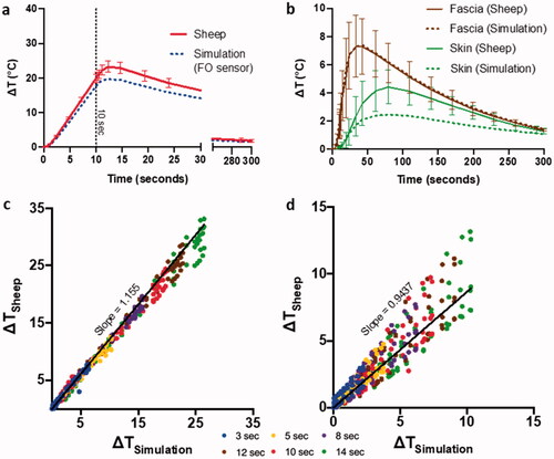
Figure 5. Validation of numerical simulations with temperature data from sheep model. Comparison of temperature evolution between simulation and sheep model for AMF heating, t_exp=10 s, on (a) implant surface, and (b) in the surrounding tissue. Summarizing the correlation between simulated temperature prediction and experimental data at multiple timepoints encompassing heating and cooldown periods for the above AMF heating for c plate sensors and d fascia and skin sensors.

Results

Simulation of plate heating with solenoid coil

The sheep leg was placed inside the solenoid (14-cm ID, 20 turns, 1 cm pitch) in the simulation model as shown in Figure 6(a) with possible directions of shift in position within the coil. The evolution of plate surface temperature distribution within the coil to the target temperature of 65 °C is shown in Figure 6(b), requiring 8 s of AMF exposure at 12 mT. The plates were heated to this temperature relatively evenly, reaching a slightly cooler temperature of 55 °C at the plate edges. The median temperature change varied less than 2 °C with translation of the implant in the coil in the x and y directions of 4 cm and ± 2 cm, respectively, as well as 5° rotation about the y axis (the maximum possible rotation of the coil with the leg inside) suggesting that AMF heating of the plate is not sensitive to these shifts in position within the coil (Figure 6(c)). Translation in the z-direction, however, produced a maximum temperature reduction of ∼15 °C with the coil translated 6 cm from its position centered on the plate.

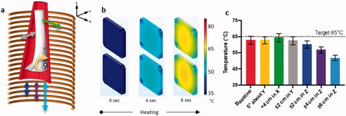
Figure 6. Simulation of sheep leg and temperature sensitivity of implant plates to movement within coil with AMF heating. Exposure duration = 8 s and T_max=65 °C. (a) The 3D simulation model showing the solenoid coil capable of producing uniform field in Z-axis, along with limb, bone, implants, axis directions and rotation about center of mass (white dot). (b) Simulated surface temperature distribution at various timepoints for AMF heating. (c) Bar graph with median and inter-quartile range for temperature distribution on the top implant plate at different positions within the coil for AMF heating.

Solenoid coil construction and characterization

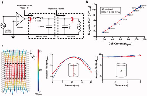
System characterization verified that experimentally determined magnetic field values matched simulations at the coil center (maximum deviation = ±0.75 mT) in both axial and radial directions and showed a linear relationship between current and magnetic field strength (Figure 7(b)). The corresponding power required to drive the circuit at each current was within the maximum operating power of 1100 W. Magnetic field characterization of the AMF system yielded a maximum amplitude of 12 mT at the coil center to a minimum of 6 mT at the coil top and bottom, as shown in Figure 7. Figure 7(c) depicts that a large central region of the coil is uniform in direction and field intensity (Figure 7(c), black dotted box). These parameters were sufficient to generate the 12 mT field to reach 65 °C on implant plates within 10–14 s for therapeutic effects as shown in in vitro studies [26,34].

Figure 7. Construction and characterization of the AMF system. (a) Circuit diagram with connections between each component of the AMF system. Function generator provides an input voltage to the amplifier. Amplified current (I₁) passes through the 50 Ω matching circuit. Current is magnified inside the tank circuit (I₂) resulting in AMF. (b) Peak magnetic field strength at coil center versus peak coil current and power delivered to the AMF system needed to generate each current (blue dots). (c) Simulation of tank circuit and the magnetic field it generates. Peak values (mT) are color-coded along magnetic field lines. Simulated and measured variation in magnetic field with change in position along coil axis and distance from center of coil.

Characterization of tissue-mimicking phantom heating profile and validation of simulations

Once the AMF system was characterized, temperature measurements of the phantom heated within the coil were performed. The simulation modeled heat accumulation within the plates, bone, and surrounding tissue (Figure 3(a)). For 60 min of intermittent AMF exposure (12 pulses, exposure duration = 14 s, pulse delay = 300 s), the heat dissipated considerably in tissue within 60 s of reaching a maximum temperature of ∼70 °C after AMF shut off. Surrounding tissues reached a maximum temperature of 45 °C within 5 mm of the surface of the plate and under 40 °C at greater distances from the plate. Plate and gel temperature measurements upon AMF exposure cycling as described above (Figure 3(b)) matched well with simulations that predicted peak temperatures within 5–10% accuracy. The plates reached a maximum temperature of 70 °C, whereas sensors in the gel placed 2 mm from the proximal plate only reached 45 °C indicating a sharp thermal gradient in tissue due to the specificity of AMF heating. As blood perfusion was not included in the simulation model, heat dissipation was incomplete over 5 min, resulting in a gradual increase in baseline temperature, both for the phantoms and simulations. Validation of simulations was performed against phantom data for different AMF exposure durations ranging from 10 to 14 s (Figure 3(c)). The simulations also predicted ΔT achieved at the center of the implant plate and gel averaged over the 12 AMF pulses delivered in 1-h, within 10–20% deviation from the experimental values for all exposure times. However, temperature measurements of the bone mimic exhibited 60–70% deviations due primarily to significant differences in the material properties from actual bone such as density and porosity of 3D printed material (refer to Appendix), as well as inaccuracy in the positioning of the fiberoptic sensor and sensitivity to positioning due to high temperature gradients.

Temperature measurements of sheep leg AMF heating of implant plate and surrounding tissue

Three sheep were used as biological replicates and the same single and multiple AMF protocols were performed on each animal. A schematic representation of the positioning of sensors on the implant plate and in the surrounding tissue (fascia and skin) is shown in Figure 4(a). The temperature data from all five sensors from a 10 s AMF single pulse (out of many single pulse exposures performed with AMF exposure times ranging from 3–14 s) with baseline implanted plate temperatures of 32°–34 °C is shown in Figure 4(c). The center of the plate had the highest heating rate with a maximum temperature rise of ∼25 °C. The temperature rise in the plate that continued beyond 10 s after power was stopped was due to sensor delay and inaccuracy of fiberoptic sensor measurement resulting from high temperature gradients at the interface between the implant plate and adjacent tissue. The temperature elevation in the adjacent fascia and skin stayed under 10° and 5° C, respectively. Discrepancies due to the response time of fiberoptic sensors was less of an issue in the surrounding tissues since the rate of heating was slower and there was a lower temperature gradient. After 5 min of cooldown, the temperature of the plate, fascia and skin returned to baseline. In a multiple pulse AMF exposure (12 pulses, 10 s duration, pulse to pulse delay = 325 s), the maximum temperatures of each heating cycle were within 5 °C of each other, as measured by the two plate sensors (Figure 4(d)). The peak temperatures were also nearly constant over the duration of the 12 pulses. In contrast to the significant baseline temperature rise in the phantom that occurred over the course of the hour-long experiment, there was a minimal rise in baseline temperature throughout the sheep leg AMF exposure due to the heat dissipation of blood perfusion.

Validation of AMF heating simulation against sheep leg and plate AMF heating

The sheep leg and metal implant temperature measurements were used to validate the simulation of the sheep leg. In Figure 5(a), AMF heating and cooldown curves for the center of the implant plate were predicted by simulation with a maximum difference of 5 °C from standard deviation (SD) of data accumulated from three sheep. The same delay of the fiberoptic sensors was observed in sheep and was precisely predicted by numerical models and was included in simulations of the sensors. Prediction of temperature curves for fascia and skin from simulations with maximum difference of 3 °C from SD of experimental data is shown in Figure 5(b). Validation of simulations was performed from single pulse AMF exposure data from sheep ranging from 3 to 14 s for plate, fascia, and skin with point-to-point comparisons of temperature profiles (Figure 5(c, d)). There was excellent correlation between the sheep leg measurements and corresponding simulations across all exposure time points. Plots of temperature measurement between the sheep experiment and simulation yielded slopes of 1.15, for plates and 0.94 for fascia and skin demonstrating strong correlation for all materials in vivo.

Due to material and response time of the fiberoptic sensors, a validated simulation model for sheep serves as a strong tool to simulate the actual temperature at the surface of an implant plate. The difference between the maximum temperatures measured by fiberoptic sensors and the surface temperatures given by simulation are presented in Table 1. An average ratio of 1.24 ± 0.03 serves as the correction factor while realizing the maximum temperature achieved by plate surface.

Table 1. To account for different in temperature measured with fiberoptic sensors to the actual temperature of the plate, a correction factor is devised.

AMF exposure (sec)	On implant surface (°C)	With FO sensor (°C)	Correction factor
3	45.0	38.4	1.17
5	51.7	42.3	1.22
8	60.1	47.7	1.26
10	65.5	51.7	1.27
12	69.0	54.7	1.26
14	73.9	58.4	1.26
Average correction factor = 1.24 ± 0.03

Simulation of thermal dose accumulation within sheep leg tissues

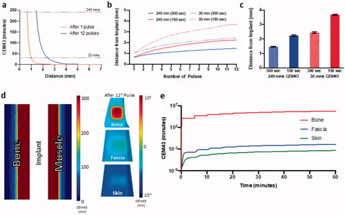
With validated simulations capable of accurately predicting temperature distribution within the implant plates and surrounding tissue, tissue damage as a function of CEM43 thermal dose was predicted and visualized. The spatial thermal dose distribution in tissue adjacent to the implant plate surface at various numbers of AMF exposures, peak temperatures, and inter-pulse delay times is shown in Figure 8. A single AMF exposure to 65 °C achieved a tissue thermal dose of 240 min CEM43 (irreversible tissue damage) <1 mm from the surface of the plate (Figure 8(a)). At 12 pulses, the 240 min CEM43 distance increased to just 1.5 mm from the plate, while the 30 min CEM43 dose (no damage) increased from 1 to 2.5 mm from the plate. For AMF exposures with a constant target plate temperature of 65 °C but decreasing the delay between pulses from 300 to 150 s (and thus the total AMF exposure time), progressive increase in thermal damage boundary is observed with each pulse (Figure 8(b)). At the end of 12th pulse, the tissue upper boundary for 240 min CEM43 increased from 1.5 to 2.2 mm, while the lower boundary for no damage (30 min CEM43), increased from 2.4 mm to almost 3.8 mm (Figure 8(c)). Hence, decreasing pulse delay increased tissue damage. The CEM43 thermal dose was calculated on various tissue surfaces including the cortical bone in direct contact with the plate, fascia (1 mm from the plate) and skin (3 mm from the plate) for multiple pulse AMF exposures (12 pulses, target = 65 °C, pulse delay = 300 s, Figure 8(d)). After 12 pulses, the cortical bone surface, which is flush with the heated implant plate received a CEM43 thermal dose of 10⁶ min, whereas fascia and skin accumulated 10⁻³min which is far below the no damage threshold (Figure 8(e)).

Figure 8. Simulation of thermal dose accumulation on and around the implant with AMF exposure. (a) Spatial distribution of CEM43 thermal dose in muscle tissue near the implant after 1 and 12 pulses of for AMF heating, T_{max, implant}=65 °C (T_i=32 °C). Thermal dose in the implant while targeting 65 °C and reducing pulse delay from 300 to 150 s (b) progressing during the 12 pulses, and (c) at the end of 12th pulse. (d) 3D thermal dose distribution on the surface and cross-section of bone, fascia, and skin (log color range) after 12 pulses of AMF heating, exposure duration = 10 s and T_{max, implant t}=65 °C. (e) Predicted evolution of thermal dose on bone, fascia and skin during corresponding to center of implant plate for the whole AMF exposure. T_i: initial temperature.

Discussion

Having proven the efficacy of AMF treatment for in-vitro studies [25] for biofilm eradication from metal surfaces, this study was designed to scale up AMF heating technology to achieve therapeutic temperatures on metal plates. These were implanted in a sheep leg and an AMF device capable of achieving parameters known from in vitro and small animal in vivo experiments to eliminate biofilm was developed. This sheep model represented a first step toward targeting human-sized anatomy and building an AMF system for it. It is also a valuable animal model for studying biofilm infection in metal implants. The system developed in this study is intended for future use in safety and efficacy studies. Hence, solenoid design used in this study is only suitable for the plate and not a complex implant. Further, as a proof-of-concept, our sheep experiments successfully indicated the tolerability of the animal under bursts of high temperatures.

With the AMF system we were able to elevate temperatures at the implant surface up to 65 °C within 20 s. The solenoid design described in this study therefore proved adequate for producing uniform magnetic fields in the axial direction and efficiently achieve high heating rates. The solenoid design was also not sensitive to implant movement up to ± 4 cm in x, y, and z directions and to rotation about the y-axis from its initial position centered on the sheep leg in simulations. This made the AMF heating less vulnerable to positional changes while preparing sheep for treatment and placing solenoid over its leg. A parallel resonant LC circuit design enabled generation of peak current upwards of 100 A to reach magnetic field strengths of up to 12 mT at the center of the coil. This helped achieve heating rates of 2.5–3 °C/s on implant plates (much higher than similar studies with large AMF coils [28,29]. In addition, water-cooling maintained component temperatures for high efficiency over long exposure times with multiple duty cycles. Electrical current and power measurements showed this system to be stable up to a maximum operating power of 1100 W (Figure 7(b)). However, the system was limited to running at maximum power for only 30 s continuously due to load capacitor (C-load) overheating even with cooling. Hence, the duty cycle was restricted to that timeframe.

The AMF heating simulations of phantom accurately predicted experimental observations from fiberoptic temperature sensors. In addition, the validated simulations enabled more detailed mapping of the three-dimensional temperature distribution. Simulations were also able to account for the lag in temperature sensor readings at the implant surface due to high thermal gradients (see Appendix) [35–49] and could predict actual temperature values on the implant surface more accurately. The simulations were further validated against in vivo experimental data from sheep leg temperature measurements. Temperature predictions were within ±5 °C. Validation of these simulations have enabled us to confidently use our computer models to predict heat transfer and thermal damage in surrounding tissue. This level of detail for the anatomy and implant otherwise would not be possible to achieve with only a few points tested with physical sensors. The importance of this experimental validation of the simulation model has also enabled us to use this platform to design AMF devices for much more complex human implants and predicting the heating of the implant surface and surrounding tissues. This platform will be vitally important in the development of AMF technology for treating such complex shaped medical implants.

These validated simulations were used to predict thermal tissue damage from variety of AMF treatment in the sheep model. This analysis revealed that number of exposures, peak temperature and delay between exposures are all important factors in determining the extent of tissue damage. While sharp gradients in thermal dose deposition can occur within the space of a few millimeters, thermal dose was concentrated just 1 to 2 mm from the implant surface. These simulations predicted highly specific heating of the implant with negligible thermal doses to surrounding tissue. This data, although presented for a simplified implanted plate geometry in sheep, is a steppingstone for future development in coil design and temperature predictions on complex human implants. To carry forward this idea, our group is currently working on developing a coil design for treating human knee implant with our understanding of simulation models presented in this study.

Finally, optimal conditions to eradicate biofilm with AMF-induced heating is an area of ongoing investigation by us and other groups. Multiple studies have confirmed that biofilm eradication is time and temperature dependent, much like eukaryotic cells. Eradication can be achieved at multiple temperatures, with less time required to reduce the burden of bacteria by a fixed amount (i.e., 3 logs) as the temperature is increased. Another important factor dictating optimal exposure conditions is the need to protect adjacent tissues from thermal damage. The longer an implant is heated, the more time there is for heat to conduct into tissue and build up to a toxic thermal dose. Our recent simulations studies on this topic (unpublished but in preparation for a manuscript) suggest that a better safety profile is achieved using high temperature (65–80 °C) for short durations (20–60 s). A recent publication from our group on in vitro biofilm [25] samples provide some insight into the effectiveness of these types of exposures.

Conclusion

Noninvasive treatment of infected orthopedic implants is a much-needed change from current standard of care. In many studies, as discussed, it has proven to be a viable approach. To treat biofilm on infected implants via heating caused due to AMF exposure is a very precise method and holds high value in biomedical industry. With our prior knowledge of in vitro and in vivo mouse AMF experiments we developed an AMF system for targeted heating of implants in a large animal model. A 3D finite element model of AMF heating was able to accurately predict the experimental measurements in a tissue-mimicking phantom and sheep leg. Based on the results of this study, it is feasible to use these simulations in the design and evaluation of future clinical AMF devices. Experiments on tissue phantoms in conjunction with simulations can also be extended to development of AMF coils for human-implants, streamlining the design process and reducing the cost and time associated with large animal studies.

Disclosure statement

Dr. David E. Greenberg and Dr. Rajiv Chopra are inventors of the technology related to AMF, holds patents related to this technology, and are the founders of Solenic Medical. Dr. David E. Greenberg serves as Chief Medical Officer and Dr. Rajiv Chopra serves as Chief Technology Officer at Solenic Medical. No potential conflict of interest was reported by the author(s).

Additional information

Funding

This work was supported by National Institute of Health (grant #1R44AI155291).

 

Appendix

A 3D finite-element model was developed to model AMF interactions with metal plates using a solenoid coil. COMSOL® Multiphysics software (COMSOL, Burlington, MA, USA) was used to calculate both the energy deposited on the metal implants from the AMF exposure, and the corresponding spatial temperature distribution by coupling a quasi-static electromagnetic model (AC/DC) with a bioheat transfer model (Heat Transfer). The coupling was only one way, thus ignored any potential thermoelectric effects. The finite element method (FEM) models were solved on a personal computer (64 GB RAM, Intel i7-9700K Processor).

3D solenoid model

A solenoid coil was modeled in COMSOL with geometries to enable current flow through the helix. This model was used with both the phantom and sheep leg model placed inside it. The coil was enclosed within a sphere to provide an air medium. A 10-mm thick layer on the surface of the sphere was created, which acted as an 'infinite boundary layer' to prevent magnetic field lines from bending unnaturally at the boundary. To connect the coil, extrude and revolve functions were used to extend end faces to form a solid cylinder of the same diameter as coil, vertically aligned with each other with a small gap in between. This gap was filled by extruding the face of one of the extended cylinders. This small cylinder served as a current source for the coil by making it a ‘lumped port’. The values used for this current were selected to match the experimental measurements of current flowing through the tank circuit. Electromagnetic properties for each component for both geometries are described in Table 1.

Table

Sphere
Constant	Value	Units
Material	Air
Diameter	400	mm
Layer thickness	10	mm
Coil
Constant	Value	Units
Material	Copper
Turns	20
Major radius (radius of the coil)	69.85	mm
Minor radius radius of the tube that makes up the coil)	3.175	mm
Axial pitch (distance between each turn)	10	mm
Lumped port
Constant	Value	Units
Material	Air
hport (Height of the cylinder)	20	mm
wport (Circumference of the cylinder)	pi*6.35	mm
Direction, ah	(0, 0, 1)	(x, y, z)
Terminal type (enables us to specify the magnitude of current)	Current
Peak terminal current (for 12.2 mT)	120	Ampere

3D Phantom/sheep leg model

3D models of a sheep leg and equivalent phantom were created in COMSOL to simulate AMF-induced heating as described in Methods section. These geometries were placed inside the solenoid coil as follows:

1. The phantom was positioned inside the coil such that the center of proximal implant plate on the bone was between 9th and 10th turn of the coil to match the location of the implants during experiments.

2. Alternatively, the sheep leg was positioned inside the coil such that the center of implant plate was at the 4th turn of the coil.

This adjustment of the plate position in the sheep leg model was necessary because the diameter of the sheep thigh only permitted insertion of the tibia this far into the coil. The sheep leg model was horizontally offset 3-cm from center to bring the plates closer to the coil windings, to match the orientation of the implant plate observed during the experiments. The offset from center was necessary due to the limited maneuverability of the leg within the coil when fully inserted during in vivo experiments. The CAD model used to produce the tibial bone in these models was obtained from CT scans of a sheep tibia (Embodi3D). The bone was segmented using (using Autodesk Meshmixer 3.5) and CAD model was created using SolidWorks 2018, (Dassault Systèmes SolidWorks Corporation, Waltham, MA, USA) and imported into COMSOL. A model of the stainless-steel plate implants with screw holes and vertical separation between plates as in the phantom was generated in SolidWorks 2018 imported into COMSOL and placed on the upper tibia as in the phantom (Figure 1). Implant screws were not modeled in the simulations due to excessive meshing required for the threads which significantly increased computational time without much impact on the temperature distribution on the plates. To model the rate of change of temperature accurately, models of the physical fiberoptic temperature sensors were included at the appropriate location in the phantom and sheep leg as described in Methods. A cylindrical volume of muscle tissue was included around the implant with the same diameter as the gel in the phantom. Whereas a conical volume was used as a more representative depiction of the animal leg. The height of muscle tissue in the simulation was reduced compared to the phantom to save computation time, but it was confirmed the reduction had no effect on the final calculated temperature distribution around the implant. Blood perfusion was included in the soft tissues in the sheep model, but not in the phantom. The physical and material properties for each component is described below:

Table

Cortical bone
Constant	Value	Units
Relative permeability	1
Electrical conductivity	0.021	S/m
Relative permittivity	205.3224
Thermal conductivity	0.32	W/(m*K)
Density	1908	kg/m^3
Heat capacity	1313	J/(kg*˚C)
Perfusion (phantom)	0	mL/min/100 g
Perfusion (sheep leg)	7.32*	mL/min/100 g
Muscle (phantom)
Constant	Value	Units
Radius	50	mm
Height	150	mm
Relative permeability	1
Electrical conductivity	0.3817	S/m
Relative permittivity	6512.674
Perfusion	0*	mL/min/100 g
Density	1090	kg/m^3
Thermal conductivity	0.49	W/(m*K)
Heat capacity	3421	J/(kg*˚C)
Muscle, fascia and skin (sheep)
Constant	Value	Units
Bottom radius	15	mm
Height	170	mm
Top radius	35	mm
Layer 1 (skin)	2.5	mm
Layer 2 (fascia)	2.5	mm
Relative permeability	1
Electrical conductivity	0.3817 (M), 0.389 (F), 0.105 (S)	S/m
Relative permittivity	6512 (M), 307 (F), 1100 (S)
Perfusion	25*(M), 0** (F), 30* (S)	mL/min/100 g
Density	1090 (M), 1027 (F), 1109 (S)	kg/m^3
Thermal conductivity	0.49 (M), 0.39 (F), 0.37 (S)	W/(m*K)
Heat capacity	3421 (M), 2372 (F), 3391 (S)	J/(kg*˚C)
316L stainless steel (implant plates)
Constant	Value	Units
Relative permeability	1.008
Electrical CONDUCTIVITY	1,351,351	S/m
Relative permittivity	1
Thermal conductivity	16.3	W/(m*K)
Density	8000	kg/m^3
Heat capacity	0.5	J/(kg*˚C)
Source for 316 L-SS constants was ASM Matweb (asm.matweb.com)
Polyimide (FO sensor outer cover)
Constant	Value	Units
Radius	0.65	mm
Height	12.5	mm
Relative permeability	1
Electrical conductivity	6.6667e-16	S/m
Relative permittivity	3.4	1
Thermal conductivity	0.12	W/(m*K)
Density	1420	kg/m^3
Heat capacity	1000	J/(kg*˚C)
Source for polyimide constants was MatWeb (www.matweb.com.)
Silica glass (FO inner sensor)
Constant	Value	Units
Radius	0.375	mm
Height	12.5	mm
Source for silica glass constants was COMSOL’s internal material library.

Note: *Blood perfusion values for sheep leg were based on an elevated blood perfusion at temperature of 45 °C (an average value for 65 °C pulse experiments) [38]. **Fascia does not have blood perfusion. Source for bone constants was IT’IS Foundation database [39]. Mesh sizes were tested with grid independency test by running the simulation for different mesh element sizes and comparing the data.

Calculations for AMF-induced power deposition on implant plates

When exposed to an alternating magnetic field (AMF), eddy currents are induced in materials based on amount of magnetic flux passing through the surface, given by Gauss’ Law for magnetism: $$\int \overrightarrow{B}\cdot d\overrightarrow{A}=0$$ where B [T] – magnetic field passing through an area A [m²].

As the frequency of the AMF is increased, the induced currents are increasingly restricted to the outer surface of the material, through a phenomenon referred to as the skin effect. The skin depth is the depth from the surface of the conductor where electrons are flowing. This is governed by Lenz’s Law and conservation of energy as a flowing charge produces its own magnetic field. The skin depth is given by the following equation: $$\delta =\sqrt{\frac{2\rho }{\omega \mu }}$$ where, δ – skin depth [m], ρ – resistivity of the conductor [Ω-m], ω – angular frequency [Hz], and µ – product of relative magnetic permeability of the conductor and the permeability of free space. The skin depth at 200 kHz for 316 L stainless steel plate is 0.97-mm.

From the above equations, the heat generated in conductor volume is given by: $$Q_r=\frac{1}{2}Re(J·E)$$ where, Q_r – heat generated due to resistive losses [W/m³], J – surface current density (calculated during simulations) [A/m²] and E – electric field [V/m]. ‘Re’ refers to the real part of the complex solution.

The heat generated by surface currents is directly proportional to electrical conductivity of the conductor. Biological tissues also have induced eddy currents and may generate heat over time; however, metal implants have much higher (>10⁶ times) electrical conductivity, rendering heat generated in tissue insignificant over the time scale of a few seconds for AMF exposures.

3D temperature and thermal dose distribution calculations

Heat transfer within the simulation volume was calculated using the bioheat transfer module in COMSOL. This module implements the Bioheat Transfer Equation (BHTE) which accounts for internal heat generation of tissue from an external source and convective heat loss due to blood perfusion. For simulations of the phantom, the perfusion was set to zero since it was a static model. In addition, a convective heat exchange boundary with surface heat transfer coefficient of 10 W/m²·K was used as an approximation on the surface interface of phantom/sheep leg with air to mimic test conditions [37,38].

The Bioheat Transfer Equation with perfusion is given by [39–43]: $$\mathrm{\rho }\mathrm{c}\frac{\partial \mathrm{T}}{\partial \mathrm{t}}=\nabla ·\left(\mathrm{k}\nabla \mathrm{T}\right)-{\omega }_b{c}_b\left(T-T_b\right)+\mathrm{ }{Q}_r+Q_m$$ where, T – temperature measured relative to core temperature [°C], t – time [s], ρ – tissue density [kg/m³], c – specific heat [J/kg°C], k – thermal conductivity [W/m/°C], ρ_b – blood density [kg/m³], c_b – blood specific heat [J/kg°C], ω_b – blood perfusion [ml/min/100g], T_b – temperature of arterial blood entering region [°C], Q_r – heat generated due to resistive losses on implant [W/m³], and Q_m – metabolic heat generation [W/m³]. In the phantom, there is no perfusion or metabolic heat generation with uniform thermal properties throughout the volume and negligible effect of electric field on tissue heating. Whereas, for sheep leg blood perfusion was added and metabolic heat was ignored as its effect was very low and negligible with the 60 min timeframe of our AMF exposures.

The temperature distributions in tissue over time are used to calculate the cumulative thermal dose using the isoeffect formulation. This enables prediction of the extent of tissue damage across a range of temperature time histories. To quantify this, CEM43 model is used. It is a method of normalization to convert the various time–temperature exposures applied into an equivalent exposure time expressed as minutes at the reference temperature of 43 °C [44]. It is defined by the following equation [45,46]: $$\mathit{CEM}43={\int }_{t_0}^{t_{\mathit{final}}}{R}^{43-T\left(t\right)}dt$$ where, R – temperature dependence of the rate of cell death (R = 0.5 for T > 43 °C, R = 0.25 for 39°C ≥ T ≥ 43 °C, and R = 0 for T < 39 °C), dt – time interval, t₀ and t_final are initial and final heating periods. This can be used to predict tissue thermal damage induced during AMF exposure. Thresholds are divided into 3 categories: (1) no damage – thermal dose is low enough to avoid damage to tissue, (2) reversible damage – thermal dose is high enough to cause some damage, but eventually cellular mechanism can heal it, and 3) irreversible damage – thermal dose is sufficiently high that irreversible tissue damage is likely [47,48]. The thresholds for reversible and irreversible tissue damage have been described based on the sensitivity of a range of tissues and organs in different species. A dose of 30 min of CEM43 was determined to cause no damage, while a > 240 min dose causes irreversible damage in muscle tissue [23,47], with skin having a slightly higher threshold at 500 min [47]. By comparison for bone, CEM43 value for reversible damage is between 80 and 1024 min and irreversible damage is beyond 2184 min [49]. These factors have been considered in the simulations to describe the safety of AMF treatment protocols and parameters.

References

- Kremers HM, et al. Prevalence of total hip and knee replacement in the United States. J Bone Joint Surg. 2014;97(17):1386–1397.
- Birlutiu RM, Birlutiu V, Mihalache M, et al. Diagnosis and management of orthopedic implant-associated infection: a comprehensive review of the literature. Biomed Res. 2017;28:5063–5073.
- Cui Q, Mihalko WM, Shields JS, et al. Antibiotic-impregnated cement spacers for the treatment of infection associated with total hip or knee arthroplasty. J Bone Joint Surg. 2007;89(4):871–882.
- Runner RP, Mener A, Roberson JR, et al. Prosthetic joint infection trends at a dedicated orthopaedics specialty hospital. Adv Orthoped. 2019;2019:1–9.
- Charette RS, Melnic CM. Two-Stage revision arthroplasty for the treatment of prosthetic joint infection. Curr Rev Musculoskelet Med. 2018;11(3):332–340.
- Luria S, Kandel L, Segal D, et al. Revision total knee arthroplasty. Israel Med Assoc J. 2003;5(8):552–555.
- Gooding CR, Masri BA, Duncan CP, et al. Durable infection control and function with the PROSTALAC spacer in two-stage revision for infected knee arthroplasty. Clin Orthopaed Relat Res. 2011;469(4):985–993.
- Fedorka CJ, Chen AF, McGarry WM, et al. Functional ability after above-the-knee amputation for infected total knee arthroplasty. Clin Orthopaed Relat Res. 2011;469(4):1024–1032.
- Kurtz SM, Lau E, Watson H, et al. Economic burden of periprosthetic joint infection in the United States. J Arthroplast. 2012;27(8 Suppl):61–65.e1.
- Pedersen AB, Mehnert F, Johnsen SP, et al. Risk of revision of a total hip replacement in patients with diabetes mellitus: a population-based follow up study. J Bone Joint Surg. 2010;92(7):929–934.
- Kurtz S, Ong K, Lau E, et al. Projections of primary and revision hip and knee arthroplasty in the United States from 2005 to 2030. J Bone Joint Surg. 2007;89:780.
- Premkumar A, et al. Projected economic burden of periprosthetic joint infection of the hip and knee in the United States. J Arthroplast. 2021;36(5):1484–1489.e3.
- Garrett TR, Bhakoo M, Zhang Z. Bacterial adhesion and biofilms on surfaces. Prog Nat Sci . 2008;18(9):1049–1056.
- Ribeiro M, Monteiro FJ, Ferraz MP. Infection of orthopedic implants with emphasis on bacterial adhesion process and techniques used in studying bacterial-material interactions. Biomatter. 2012;2(4):176–194.
- Rasmussen RM, Epperson RT, Taylor NB, et al. Plume height and surface coverage analysis of methicillin-resistant Staphylococcus aureus isolates grown in a CDC biofilm reactor. Biofouling. 2019;35(4):463–471.
- Al-Ahmad A, et al. Biofilm formation and composition on different implant materials in vivo. J Biomed Mater Res. 2010; 95(1):101–109.
- Larimer C, Suter JD, Bonheyo G, et al. In situ non-destructive measurement of biofilm thickness and topology in an interferometric optical microscope. J Biophoton. 2016;9(6):656–666.
- Donlan RM. Biofilms: microbial life on surfaces. Emerg Infect Dis. 2002;8(9):881–890.
- Gielen FLH, Wallinga-de Jonge W, Boon KL. Electrical conductivity of skeletal muscle tissue: Experimental results from different muscles in vivo. Med Biol Eng Comput. 1984;22(6):569–577.
- Yang L, Yu H, Jiang L, et al. Improved anticorrosion properties and electrical conductivity of 316L stainless steel as bipolar plate for proton exchange membrane fuel cell by lower temperature chromizing treatment. J Power Sources. 2010;195(9):2810–2814.
- Soetaert F, Korangath P, Serantes D, et al. Cancer therapy with iron oxide nanoparticles: agents of thermal and immune therapies. Adv Drug Deliv Rev Vols. 2020;163–164:65–83.
- Wentworth SM, Baginski ME, Faircloth DL, et al. Calculating effective skin depth for thin conductive sheets. 2006 IEEE Antennas and Propagation Society International Symposium, 2006. pp. 4845–4848
- Weinberg IN, Stepanov PY, Fricke ST, et al. Increasing the oscillation frequency of strong magnetic fields above 101 kHz significantly raises peripheral nerve excitation thresholds. Med Phys. 2012;39(5):2578–2583.
- Sadaphal V, Mukherjee S, Ghosh S. Hybrid photomagnetic modulation of magnetite/gold-nanoparticle-deposited dextran-covered carbon nanotubes for hyperthermia applications. Appl Phys Express. 2018;11(9):097001.
- Wang Q, Vachon J, Prasad B, et al. Alternating magnetic fields and antibiotics eradicate biofilm on metal in a synergistic fashion. Npj Biofilms Microbiomes. 2021;7(1):1–10.
- Chopra R, Shaikh S, Chatzinoff Y, et al. Employing high-frequency alternating magnetic fields for the non-invasive treatment of prosthetic joint infections. Sci Rep. 2017;7(1):7520.
- Pijls BG, Sanders IMJG, Kuijper EJ, et al. Segmental induction heating of orthopaedic metal implants. Bone Joint Res. 2018;7(11):609–619.
- Stauffer PR, Cetas TC, Jones RC. Magnetic induction heating of ferromagnetic implants for inducing localized hyperthermia in Deep-Seated tumors. IEEE Trans Biomed Eng. 1984;31(2):235–251.
- Stauffer PR, Sneed PK, Hashemi H, et al. Practical induction heating coil designs for clinical hyperthermia with ferromagnetic implants. IEEE Trans Biomed Eng. 1994;41(1):17–28.
- Stauffer PR, Cetas TC, Fletcher AM, et al. Observations on the use of ferromagnetic implants for inducing hyperthermia. IEEE Trans Biomed Eng. 1984;31(1):76–90.
- Williams DL, Woodbury KL, Haymond BS, et al. A modified CDC biofilm reactor to produce mature biofilms on the surface of PEEK membranes for an in vivo animal model application. Curr Microbiol. 2011;62(6):1657–1663.
- Williams DL, et al. Experimental model of biofilm implant-related osteomyelitis to test combination biomaterials using biofilms as initial inocula. J Biomed Mater Res A. 2012;100(7):1888–1900.
- Chen RK, Shih AJ. Multi-modality gellan gum-based tissue-mimicking phantom with targeted mechanical, electrical, and thermal properties. Phys Med Biol. 2013; 58(16):5511–5525.
- Cheng B, Chatzinoff Y, Szczepanski D, et al. Remote acoustic sensing as a safety mechanism during exposure of metal implants to alternating magnetic fields. PLOS One. 2018;13(5):e0197380.
- Song CW. Effect of local hyperthermia on blood flow and microenvironment: a review. Cancer Research. 1984;44(10 Suppl):4721s–4730s.
- Hasgall PA, Di Gennaro F, Baumgartner C, et al. IT’IS database for thermal and electromagnetic parameters of biological tissues, version 4.0. IT’IS; 2018. https://doi.org/10.13099/VIP21000-04-0
- Prasad B, Kim S, Cho W, et al. Effect of tumor properties on energy absorption, temperature mapping, and thermal dose in 13.56-MHz radiofrequency hyperthermia. J Therm Biol. 2018;74:281–289.
- Hossain MT, Prasad B, Park KS, et al. Simulation and experimental evaluation of selective heating characteristics of 13.56 MHz radiofrequency hyperthermia in phantom models. Int J Precis Eng Manuf. 2016;17(2):253–256.
- Strohbehn JW. Theoretical temperature distributions for solenoidal-type hyperthermia systems. Med Phys. 1982;9(5):673–682.
- Kok HP, van der Zee J, Guirado FN, et al. Treatment planning facilitates clinical decision making for hyperthermia treatments. Int J Hyperthermia. 2021;38(1):532–551.
- Gavazzi S, van Lier ALHMW, Zachiu C, et al. Advanced patient-specific hyperthermia treatment planning. Int J Hyperthermia. 2020;37(1):992–1007.
- Liu D, Adams MS, Diederich CJ. Endobronchial high-intensity ultrasound for thermal therapy of pulmonary malignancies: simulations with patient-specific lung models. Int J Hyperthermia. 2019;36(1):1107–1120.
- Pennes HH. Analysis of tissue and arterial blood temperatures in the resting human forearm. J Appl Physiol. 1948;1(2):93–122.
- Van Rhoon GC. Is CEM43 still a relevant thermal dose parameter for hyperthermia treatment monitoring? Int J Hyperthermia. 2016;32(1):50–62.
- Pearce JA. Comparative analysis of mathematical models of cell death and thermal damage processes. Int J Hyperthermia. 2013;29(4):262–280.
- Nadobny J, Klopfleisch R, Brinker G, et al. Experimental investigation and histopathological identification of acute thermal damage in skeletal porcine muscle in relation to whole-body SAR, maximum temperature, and CEM43 °C due to RF irradiation in an MR body coil of birdcage type at 123 MHz. Int J Hyperthermia. 2015;31(4):409–420.
- van Rhoon GC, Samaras T, Yarmolenko PS, et al. CEM43 °C thermal dose thresholds: a potential guide for magnetic resonance radiofrequency exposure levels? Eur Radiol. 2013;23(8):2215–2227.
- Pearce JA. Relationship between Arrhenius models of thermal damage and the CEM 43 thermal dose. Proceedings Volume 7181, Energy-based Treatment of Tissue and Assessment V, 718104; 2009
- Burtnyk M, Chopra R, Bronskill M. Thermal analysis of the surrounding anatomy during 3-D MRI-guided transurethral ultrasound prostate therapy. AIP Conference Proceedings, vol. 1215; 2010;26(8):804–821.