A visualization method for a wide range of rising temperature induced by high-intensity focused ultrasound using a tissue-mimicking phantom

Abstract

Purpose

High-intensity focused ultrasound (HIFU) treatment requires prior evaluation of the HIFU transducer output. A method using micro-capsulated thermochromic liquid crystal (MTLC) to evaluate the temperature distribution in the media during HIFU exposure has been previously developed. However, the color-coded temperature range of commercial MTLC is approximately 10 °C, which is insufficient for temperature measurement for HIFU exposure. We created two layers of tissue-mimicking phantoms with different color-coded temperature ranges, and a new visualization method was developed by utilizing the axisymmetric pressure distribution of a HIFU focus.

Methods

A two-layer phantom with two sensitivity ranges was created. The HIFU transducer was set to align the focal point to the boundary between the two layers. Images of the upper and lower layers were flipped along the boundary between the two layers such that they overlapped with each other, assuming the pressure distribution of HIFU to be axisymmetric.

Results

The experimental and simulation results were compared to evaluate the accuracy of the phantom temperature measurement. The experimental time profile of the temperature and spatial distribution around the HIFU focus matched well with that of the simulation. However, there is room for improvement in the accuracy in the axial direction of HIFU focus.

Conclusion

Users can apply our proposed method in clinical practice to promptly assess the output of the HIFU transducer before treatment.

Keywords:

• High-intensity focused ultrasound
• noninvasive thermometry
• ultrasound phantom
• tissue-mimicking phantom
• principal component analysis (PCA)
• pressure measurement

1. Introduction

High-intensity focused ultrasound (HIFU) treatment [1–5] is a non-invasive method for ablating various tumors such as prostate [6,7], breast [8,9], liver [10,11], pancreas [12,13], and brain [14], therefore, the output produced by the HIFU transducer should be checked before treatment. When the elements of the HIFU array transducer are partially or totally damaged, the HIFU acoustic pressure field is distorted and exhibits inadvertent focus on normal healthy tissue.

Recently, numerical simulations of ultrasound propagation, using finite difference time domain (FDTD) methods, were investigated to estimate the HIFU focal region and correct the focal errors of beamforming in heterogeneous tissues and deep tissue cancers (brain tumors and liver cancer [15,16]. In order to use this FDTD technique, bone the structure and acoustic property data are obtained using magnetic resonance imaging (MRI) or X-ray computed tomography, and the distortion of HIFU focus is corrected using the time-reversal approach [17], which is an adaptive technique for correcting phase aberrations induced by a medium’s acoustic heterogeneities. Focal errors of the HIFU beam in the tissues can be effectively decreased by using the FDTD method, which is applicable only if the HIFU transducer elements are not damaged and are operated under normal conditions. Therefore, it is necessary to experimentally investigate the reliability of the therapeutic device in actual clinical practice before HIFU treatment.

There are two approaches for investigating the output of a therapeutic device before treatment. First, the measurement of the acoustic pressure field or acoustic power; second, the measurement of the temperature distribution induced by the HIFU using a tissue-mimicking medium.

An acoustic pressure induced by a therapeutic device in water is commonly measured using a hydrophone, which is scanned mechanically through the water to measure a two or three-dimensional (2-D or 3-D) acoustic pressure field. Hydrophone measurements of the 2-D or 3-D acoustic pressure field are time-consuming. The acoustic power can be measured by a radiation force balance, but the distribution of an acoustic pressure field cannot be measured.

Optical-based acoustic pressure field mapping using a schlieren system [18,19] requires less time and does not interfere with the acoustic field. However, the system is relatively large and complicated for use in clinical practice.

Temperature distribution is typically measured using thermocouples [20], which are inserted into the tissue-mimicking medium. Many thermocouples are needed to measure the 2-D temperature distribution; this affects the thermal conditions inside the medium, and thus produces measurement artifacts. MRI thermometry [21] is a promising method for measuring temperature distribution; nevertheless, it is expensive and lacks portability, and all experimental systems – including the therapeutic device – must be MRI compatible.

A visualization method using micro-capsulated thermochromic liquid crystal (MTLC) for temperature distribution measurement was proposed in a previous study [22]. In this method, MTLC was mixed with a transparent urethane material, and the temperature increase during HIFU exposure was visualized by utilizing the thermometric property wherein the optical reflectance spectrum of MTLC changes according to the temperature. The proposed system is relatively simple (consisting of a tissue-mimicking material, light source, and optical camera) and seemingly suitable for use in clinical practice. However, the visualized temperature range was only 10 °C because the color-coded temperature of commercial MTLC ranged from 1 to 10 °C. Thermometery with a temperature range of 10 °C cannot be used to measure the temperature rise in a medium during HIFU exposure, which typically induces a 20–40 °C temperature rise [1,2].

In this study, a two-layer-tissue-mimicking phantom with different color-coded temperature ranges was created, and a new visualization method utilizing an axisymmetric focal pressure distribution of HIFU was developed to measure a wider range of temperature rise during HIFU exposure. The experimental results were compared with the simulation results to verify the accuracy of the proposed method.

2. Materials and methods

2.1. Concept of the proposed method

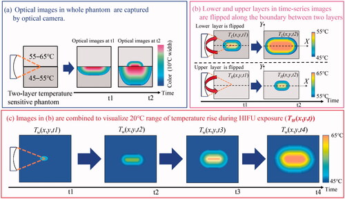
Figure 1 illustrates the concept of the proposed method. It achieved a sensitive temperature range that was wider than the conventional range. Two types of temperature-sensitive phantoms with sensitivities ranging from 45 to 55 °C and from 55 to 65 °C were produced, as lower and higher layers, respectively. In this study, the higher and lower temperature-sensitive phantoms were defined as ‘H-phantom’ and ‘L-phantom’, respectively.

Figure 1. (a–c) Concept of the proposed method, which achieves a wider sensitive temperature range than the conventional range.

A spherical HIFU transducer was set such that the HIFU focal point was aligned to the boundary between the H-phantom and L-phantom. To align the HIFU focus to the boundary of the phantoms before the temperature measurement, the HIFU transducer was moved manually while 1-ms low-intensity (approximately 1 W) ultrasound pulse was transmitted with a repetition period of 10 ms until the boundary of the phantoms became colored.

Figure 1 illustrates the side view of the experimental setup. The axial and lateral axes of the HIFU transducer were set as the X- and Y-axes, respectively.

As shown in Figure 1(a), the optical images of the L- and H-phantoms were captured using the optical camera following HIFU exposure initiation. The L-phantom color initially changed as the temperature increased because the temperature-sensitive range of the L-phantom was lower than that of the H-phantom. The H-phantom color changed after the temperature of the focal area exceeded 55 °C.

As shown in Figure 1(b), the lower and upper optical images in the entire time series are flipped along the axial direction of the HIFU transducer (the boundary between the two layers) to obtain the 2-D temperature distribution, which assumes that the pressure distribution of the HIFU is axisymmetric. The 2-D-reflected color information is converted to temperature by calibration processing of the optical images, as explained in Section 2.4, to obtain the increase in the lower and higher temperatures corresponding to the HIFU exposure duration. The 2-D lower and higher temperature distribution in a time series is described as T_L(x,y,t) and, T_H(x,y,t) respectively, where x, y, and t indicate the axial pixels of the phantom, lateral pixels of the phantom, and HIFU exposure time, respectively.

As shown in Figure 1(c), the maximum value was selected from the pixels in T_L and T_H at each time series to obtain a wider range of temperature distribution (T_W) for the duration of HIFU exposure; the background pixels (no color region) in T_H was set to 45 °C, not 55 °C.

2.2. Two-layer temperature-sensitive phantom

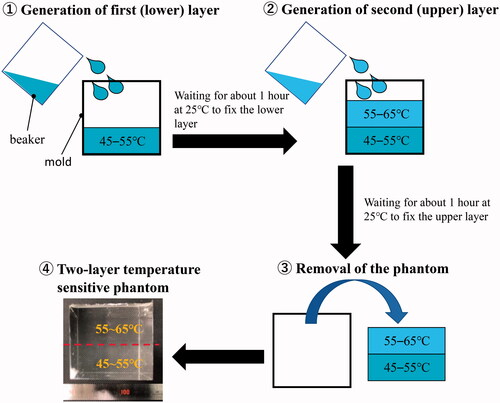
In this study, a urethane material (H05, Exseal Corporation, Gifu, Japan) was used to produce the tissue-mimicking phantom because the material is transparent and colorless, and thus, suitable for optical color measurement. It also has heat-resistant properties, which means that the HIFU exposure experiment can be conducted repeatedly with the same phantom, which makes it suitable for use in clinical practice. The diameter of the MTLC (Japan Capsular Products, Tokyo, Japan) was approximately 30 μm. The urethane phantom had an MTLC concentration of 0.005%. The density of the phantom ranged from 1052 ± 7.1 to 1054 ± 7.8 kg/m³. Figure 2 shows the procedure for the creation of the two-layer temperature-sensitive phantom. First, a material with a temperature-sensitive range of 45–55 °C was poured into the mold to generate the first layer (L-phantom). The size of the mold was 50 × 50 × 50 mm. Then, another material with a temperature-sensitive range of 55–65 °C was poured into the mold to generate the second layer (H-phantom). After waiting for approximately 1 h at 25 °C to allow the H-phantom to adhere to the L-phantom, the fixed two-layer phantom was removed from the mold.

Figure 2. Procedure for creation of the two-layer temperature-sensitive phantom.

Table 1 shows the thermal and acoustic properties of L- (a) and H-phantoms (b). There were five samples of both the temperature-sensitive phantoms.

Table 1. Thermal and acoustic properties of the phantoms.

L-phantom (45–55 °C)	n = 5
H-phantom(55–65 °C)
Density [kg/m^3]	1054 ± 7.1
Speed of sound [m/s]	1420 ± 3.5
Attenuation coefficient [dB/MHz/cm]	1.5 ± 0.09
Specific heat capacity [J/(kg K)]	2227 ± 4.0
Thermal conductivity [W/(m K)]	0.020 ± 0.002
Density [kg/m^3]	1052 ± 7.8
Speed of sound [m/s]	1421 ± 3.8
Attenuation coefficient [dB/MHz/cm]	1.2 ± 0.06
Specific heat capacity [J/(kg K)]	2230 ± 5.5
Thermal conductivity [W/(m K)]	0.021 ± 0.003

The densities of the samples were measured using the Archimedes method. The specific heat capacity and thermal conductivity were measured using the differential scanning calorimetry [23] and hot wire methods [24], respectively. The speed of sound and attenuation in the phantom were measured and calculated using the following procedure.

Two single-element transducers with the same resonance frequency were used as a transmitter (Tr1) and a receiver (Re1) in water. First, the time of flight with no sample (T₀) was measured, and the speed of sound ($V_w$) was calculated using Equation (1)(1) $$V_w=\frac{D_0}{T_0}$$(1) after measuring $D_0$ which is the distance between the transmitter and receiver. (1) $$V_w=\frac{D_0}{T_0}$$(1)

Second, a sample with a thickness of $D_1$ was inserted in the water, and the time of flight ($T_1$) between Tr1 and Re1 was measured. $T_1$ was described as Equation (2)(2) $$T_1=\frac{D_0-D_1}{V_w}+\frac{D_1}{V_1}$$(2) : (2) $$T_1=\frac{D_0-D_1}{V_w}+\frac{D_1}{V_1}$$(2) where, $V_1$ is the speed of sound in the sample. The time difference ($\Delta T_1$) between $T_1$ and $T_0$ was calculated using Equation (3)(3) $$\Delta T_1=\mathrm{ }{T}_1-T_0=\mathrm{ }{D}_1\mathrm{ }\left(\frac{1}{V_1}-\frac{1}{V_w}\right)$$(3) : (3) $$\Delta T_1=\mathrm{ }{T}_1-T_0=\mathrm{ }{D}_1\mathrm{ }\left(\frac{1}{V_1}-\frac{1}{V_w}\right)$$(3)

Third, Tr1 was used as both a transmitter and receiver. The time interval ($\Delta T_2$) between front and back surface echoes received by Tr1 was measured. $\Delta T_2$ was described as Equation (4)(4) $$\Delta T_2=\mathrm{ }\frac{2D_1}{V_1}$$(4) : (4) $$\Delta T_2=\mathrm{ }\frac{2D_1}{V_1}$$(4)

The speed of sound in the sample ($V_1$) was calculated with measurable parameters of $V_w,$ $\Delta T_1$ and $\Delta T_2$ using Equation (5)(5) $$V_1=\mathrm{ }{V}_w\mathrm{ }\left(\frac{2\Delta T_1}{\Delta T_2}-1\right)$$(5) from Equations (3)(3) $$\Delta T_1=\mathrm{ }{T}_1-T_0=\mathrm{ }{D}_1\mathrm{ }\left(\frac{1}{V_1}-\frac{1}{V_w}\right)$$(3) and (4)(4) $$\Delta T_2=\mathrm{ }\frac{2D_1}{V_1}$$(4) : (5) $$V_1=\mathrm{ }{V}_w\mathrm{ }\left(\frac{2\Delta T_1}{\Delta T_2}-1\right)$$(5)

In order to measure the attenuation of the sample, the amplitude of tone burst waveform transmitted by Tr1 was compared with that received by Re1. Tr1 was aligned to Re1 to maximize the received signal before inserting the sample into the water. The difference in the amplitude between the transmitted and received waves without a sample corresponding to the attenuation of water. The frequency-dependent attenuation coefficient $\alpha (f)$ of the sample was calculated using the amplitude of the received signals with ($A_1\left[f\right]$) and without ($A_0\left[f\right]$) sample, as shown in Equation (6)(6) $$\alpha \left(f\right)=\frac{-\ln \left(\frac{A_1\left[f\right]}{A_0\left[f\right]T}\right)}{D_1}$$(6) : (6) $$\alpha \left(f\right)=\frac{-\ln \left(\frac{A_1\left[f\right]}{A_0\left[f\right]T}\right)}{D_1}$$(6)

$T$ is the transmission factor and is calculated using Equation (7)(7) $$T=\frac{4Z_w{Z}_1}{{(Z_w+Z_1)}^2}$$(7) as follows: (7) $$T=\frac{4Z_w{Z}_1}{{(Z_w+Z_1)}^2}$$(7) where, $Z_w$ and $Z_1$ are the acoustic impedances of water and the sample, respectively.

In this study, it was found that the attenuation coefficient increased linearly with the frequency range from 1 to 7 MHz upon using the elements with the same frequency range. The attenuations of the phantoms were 1.5 ± 0.09 (L-phantom) and 1.2 ± 0.06 (H-phantom) [dB/MHz/cm]. Moreover, the attenuation of water was 2.2 × 10⁻³ [dB/MHz/cm].

As shown in Table 1, differences in the thermal properties between the two phantoms were observed, and small heat transfer is assumed to have occurred at the boundary between the two different layers. The actual temperature increase in the tissue could not be simulated in this experiment because the phantom thermal conductivity was much less than that of the tissue. However, it is assumed that the difference in thermal properties between the tissue and the phantom has little effect on the verification of the therapeutic device output.

2.3. Experimental setup

Figure 3 shows the top (a) and side (b) views of the experimental setup. A light sheet produced by a xenon slit light source (KS-150-100, KATO KOKEN, Kanagawa, Japan) was illuminated by the phantoms to measure the 2-D temperature distribution. The thickness of the light sheet was 3.0 mm. The illuminated sections were captured using a CMOS camera (STC-MCCM200U3V, OMRON SENTECH, Kanagawa, Japan) with an optical exposure time of 80 ms. The frame rate of optical imaging was 10 fps.

Figure 3. Experimental setup: (a) top view and (b) side view.

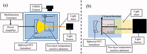
The HIFU was generated by a single-element spherical PZT transducer (Fuji Ceramics, Shizuoka, Japan) with a focal length of 46 mm, an aperture diameter of 46 mm, and a driving frequency of 1.73 MHz. A multifunction generator (WF1974, NF Corporation, Kanagawa, Japan) generated the driving signal, which was amplified by an RF amplifier (2100 L, Electronics & Innovation Ltd, NY, USA). The phantoms were placed in a sample holder, and the HIFU focal spot was targeted toward the phantoms 10 mm from the surface. The phantom was exposed to HIFU for 30 s with an acoustic power of 2.5 W, which was estimated from the focal pressure measured using a hydrophone (NH0200, Precision Acoustics Ltd, Dorchester, UK) at a low power level by assuming a quadratic relation between the amplifier output voltage and the acoustic power. The acoustic power used in this study (2.5 W) was relatively less than that of the actual HIFU treatment to prevent cavitation and boiling in the phantoms during HIFU exposure. The objective of this study was to verify the output of the HIFU transducer, which does not necessarily have the same acoustic power as that of the actual HIFU treatment.

The HIFU exposure experiment was conducted once with five different lot samples to investigate the reproducibility of our proposed method. A tank was filled with deionized water and kept at 36 °C with a dissolved oxygen content of 2.1–2.7 mg/L.

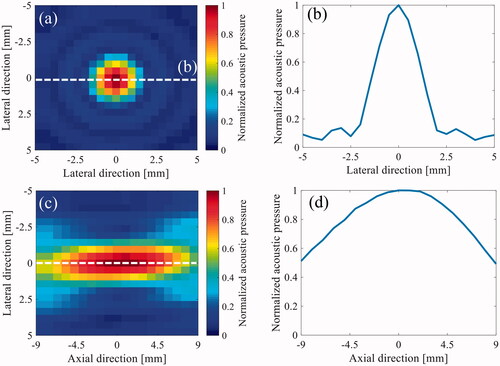
Figure 4 shows the normalized 2-D HIFU focal pressure profiles for both the transverse (a) and axial-lateral (c) planes and the one-dimensional (1-D) beam profile along the lateral (b) and axial (d) directions, with an acoustic power of 0.3 W measured using the needle hydrophone. The −6 dB longitudinal and lateral focal widths were 18 and 1.8 mm, respectively.

Figure 4. Normalized two-dimensional high intensity focused ultrasound (2-D HIFU) focal pressure profiles in both (a) the transverse and (c) axial-lateral planes and one-dimensional(1-D) beam profiles along both (b) the lateral and (d) axial directions.

2.4. Calibration process

The relationship between the reflected color information and temperature was investigated for conversion of the phantom color into temperature before all the HIFU exposure experiments. Two pairs of two-layer temperature-sensitive phantoms were produced in each lot. One was for calibration, to evaluate the relationship between color and temperature; the other was for the HIFU exposure experiment. Figure 5 illustrates the calibration process. A 0.3 mm sheath thermocouple (K-type, SUS316 sheath, CHINO, Tokyo, Japan) was inserted into the upper and lower layers of the phantom. The phantom was placed in a thermostatic chamber (SOFW-300S, AS ONE, Tokyo, Japan) and heated to approximately 80 °C (Figure 5(a)).

Figure 5. (a,b) Diagram of the calibration process.

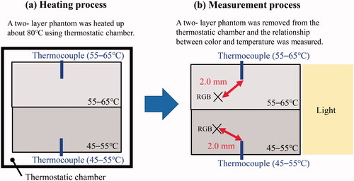
The phantom with thermocouples was taken from the thermostatic chamber and immediately placed into the water tank to evaluate the relationship between the phantom color and the temperature decrease from 80 to 45 °C. The red, green, and blue (RGB) values were obtained 2.0 mm away from the thermocouple to reduce the effect of shadow and light reflection by the thermocouples (Figure 5(b)).

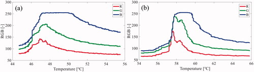
Figure 6 shows an example of the relationship between the RGB values in the optical images and temperature in the lower (a) and upper (b) layers.

Figure 6. An example of the relationship between the red, green, and blue (RGB) values in the optical images and the temperature in the (a) lower layer (45–55 °C) and (b) upper layer (55–65 °C).

In order to construct a table presenting the relationship between color and temperature, the principal component analysis (PCA) [25] was applied to the measured RGB values corresponding to the temperature values (described in a previous study [22]). PCA is a dimensional reduction technique that is commonly used in exploratory data analysis [25].

As described in Equation (8)(8) $$\mathit{C}=\left(\begin{array}{ccc}{c}_{11}& \cdots & c_{p1}\\ ⋮& \ddots & ⋮\\ c_{n1}& \cdots & c_{pn}\end{array}\right)$$(8) , C is defined as an (n × p) matrix, where each of the p columns and n rows obtained R, G, and B values corresponding to the temperature and number of pixels in the optical images, respectively. The parameters of p and n were set to 3 (R, G and B values) and 769,104, respectively (the number of pixels in axial and lateral directions were 1008 and 763 pixels, respectively). (8) $$\mathit{C}=\left(\begin{array}{ccc}{c}_{11}& \cdots & c_{p1}\\ ⋮& \ddots & ⋮\\ c_{n1}& \cdots & c_{pn}\end{array}\right)$$(8)

PCA projects p-dimensional data into a q-dimensional space (q $\le$ p). A projected vector with a principal component score ${\mathit{Y}}_{\mathit{k}(\mathit{i})}$ (i, k: natural number) was described as follows: (9) $${\mathit{Y}}_{k\left(i\right)}{=\mathit{c}}_{\left(i\right)}·{\mathit{w}}_{\left(k\right)} \mathrm{for}\mathrm{ }i\mathrm{ }=\mathrm{ }1,\mathrm{ }2,\mathrm{ }\dots n,\mathrm{ }k\mathrm{ }=\mathrm{ }1,\mathrm{ }2,\mathrm{ }\dots q$$(9)

Here, ${\mathit{c}}_{(i)}$ and ${\mathit{w}}_{\left(k\right)}={({\mathit{w}}_1,\dots \dots ,{\mathit{w}}_p)}_{(k)}$ represented each row vector of C with a set of size q of p-dimensional vectors of weight. The first weight vector ${\mathit{w}}_{\left(1\right)}$ was determined by maximizing the sum of the squared principal components (${\mathit{Y}}_{1(i)}$), as shown in Equation (10)(10) $$=\mathrm{arg }\mathit{max}\left\{\frac{{\mathit{w}}^T·{\mathit{C}}^T·\mathit{C}·\mathit{w}}{{\mathit{w}}^T·\mathit{w}}\right\}$$(10) , where $\mathit{w}$ is constrained as a unit vector. $${\mathit{w}}_{\left(1\right)}={\mathrm{arg }\mathit{max}}_{\Vert \mathit{w}\Vert =1}\left\{{\sum }_{i=1}^n{\left({\mathit{Y}}_{1\left(i\right)}\right)}^2\right\}={\mathrm{arg }\mathit{max}}_{\Vert \mathit{w}\Vert =1}\left\{{\sum }_{i=1}^n{\left({\mathit{c}}_{\left(i\right)}·{\mathit{w}}_{\left(1\right)}\right)}^2\right\}$$ $$={\mathrm{arg }\mathit{max}}_{\Vert \mathit{w}\Vert =1}\left\{\Vert {\mathit{w}}^T·{\mathit{C}}^T·\mathit{C}·\mathit{w}\Vert \right\}$$ (10) $$=\mathrm{arg }\mathit{max}\left\{\frac{{\mathit{w}}^T·{\mathit{C}}^T·\mathit{C}·\mathit{w}}{{\mathit{w}}^T·\mathit{w}}\right\}$$(10) ${\mathit{c}}_{\left(i\right)}$ was given a first principal component score ${\mathit{Y}}_{1\left(i\right)}{=\mathit{c}}_{\left(i\right)}·{\mathit{w}}_{\left(1\right)}$ in the transformed coordinate. The k-th component was determined by subtracting the first k − 1 principal components from the original data matrix C. (11) $${{\mathit{C}}^{\mathrm{\text{'}}}}_k=\mathit{C}-{\sum }_{i=1}^{k-1}\mathit{C}·{\mathit{w}}_{\left(\mathit{i}\right)}·{\mathit{w}}_{\left(\mathit{i}\right)}^T$$(11)

The k-th weight vector was derived from the maximum variance using the new data matrix (${{\mathit{C}}^{\text{'}}}_{\mathit{k}}$), as described in Equation (12)(12) $${\mathit{w}}_{\left(k\right)}={\mathrm{arg }\mathit{max}}_{\Vert \mathit{w}\Vert =1}\left\{{\Vert {\mathit{C}\text{'}}_k·\mathit{w}\Vert }^2\right\}=\mathrm{arg }\mathit{max}\left\{\frac{{\mathit{w}}^T·{\mathit{C}\text{'}}^T·\mathit{C}\text{'}·\mathit{w}}{{\mathit{w}}^T·\mathit{w}}\right\}$$(12) . (12) $${\mathit{w}}_{\left(k\right)}={\mathrm{arg }\mathit{max}}_{\Vert \mathit{w}\Vert =1}\left\{{\Vert {\mathit{C}\text{'}}_k·\mathit{w}\Vert }^2\right\}=\mathrm{arg }\mathit{max}\left\{\frac{{\mathit{w}}^T·{\mathit{C}\text{'}}^T·\mathit{C}\text{'}·\mathit{w}}{{\mathit{w}}^T·\mathit{w}}\right\}$$(12)

${\mathit{Y}}_{\mathit{k}\left(\mathit{i}\right)}{=\mathit{c}}_{\left(i\right)}·{\mathit{w}}_{\left(k\right)}$ was the k-th component score in the transformed coordinate, which is projected from the original coordinate.

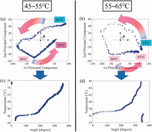
Figure 7(a,b) illustrate an example of the 2-D projected plane defined by the 1st and 2nd principal component after applying the PCA to RGB values in the lower and upper layers. The projected data points moved counterclockwise as the temperature increased. The center of gravity was estimated using the projected data points, and the projected 2-D plane was transformed into a polar coordinate, where the estimated center of gravity of data was defined as the (0,0) position. The phases of the plotted data points were calculated in the transformed polar coordinate such that the table presented the relationship between the color data and temperature. Figure 7(c,d) shows the relationship between the phase angle and the temperature in the lower and upper layers. Figure 7(c,d) were used as calibration curves because the phase angle changed as the temperature increased.

Figure 7. An example of the two-dimensional (2-D) projected plane defined by the 1st and 2nd principal component after applying the principal component analysis (PCA) to the red, blue, and green (RGB) values in the (a) lower (45–55 °C) and (b) upper (55–65 °C) layers. Relationship between the phase angle and temperature in the (c) lower (45–55 °C) and (d) upper (55–65 °C) layers.

The 2-D temperature distribution was obtained by applying the abovementioned calibration process to the original optical images. A median filter with a window size of 1.0 × 1.0 mm was applied to the acquired temperature distribution to smoothen the images.

2.5. Acoustic and thermal simulation

In this study, the experimental results using the two-layer temperature-sensitive phantom were compared with the simulation results to evaluate the accuracy of the temperature rise in the concerned phantom. Acoustic and thermal simulations were performed using the open-source k-Wave toolbox [26,27], which is implemented in MATLAB™ (MathWorks, Massachusetts, USA) to verify the accuracy of the proposed method. In this simulation, the ultrasound propagation media were water and urethane. The speed of the sound and density of water was set to 1420 and 1050 kg/m³, respectively. A k-Wave toolbox treats the medium as a sound-absorbing fluid in which the absorption follows a frequency power law of the form (13) $$\alpha =\mathrm{ }{\alpha }_0{f}^y,$$(13) where $\alpha ,$ ${\alpha }_0,$ f, and y are the absorption coefficient, power-law prefactor, frequency, and law exponent, respectively. y was set to 1.0, and the ${\alpha }_0$ of water and urethane were set to 2.2 × 10⁻³ and 1.5 dB MHz^−y cm⁻¹ in this simulation. Other thermal and acoustic properties of the urethane material were set according to Table 1. The thermal simulation was performed with the following bio-heat transfer equation (BHTE) [28,29]. (14) $$\rho C_P\frac{\partial T}{\partial t}=k\left(\frac{{\partial }^{2}T}{\partial x^2}+\frac{{\partial }^{2}T}{\partial y^2}+\frac{{\partial }^{2}T}{\partial z^2}\right)+2\alpha I-W_b{C}_b(T-T_b),$$(14) where T, t, ρ, C_P, k, $\alpha ,$ I, W_b, C_b, and T_b are the temperature, time, density, specific heat capacity, thermal conductivity, ultrasonic absorption coefficient, the intensity of ultrasound, blood volume, specific heat capacity of the blood, and blood temperature, respectively. In this study, $W_b{C}_b(T-T_b)$ was neglected because there was no blood flow in the phantom. Therefore, Equation (15)(15) $$\rho C_P\frac{\partial T}{\partial t}=k\left(\frac{{\partial }^{2}T}{\partial x^2}+\frac{{\partial }^{2}T}{\partial y^2}+\frac{{\partial }^{2}T}{\partial z^2}\right)+2\alpha I,$$(15) was used in the simulation as follows. (15) $$\rho C_P\frac{\partial T}{\partial t}=k\left(\frac{{\partial }^{2}T}{\partial x^2}+\frac{{\partial }^{2}T}{\partial y^2}+\frac{{\partial }^{2}T}{\partial z^2}\right)+2\alpha I,$$(15)

The initial temperature of the phantom and water before HIFU exposure was set to 36 °C.

3. Results

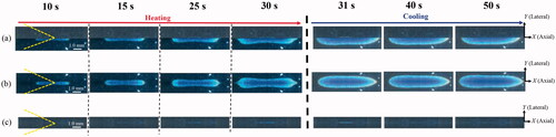
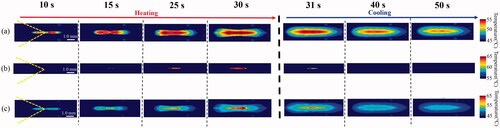
Figure 8(a) shows an example of the original optical images of the two-layer phantom during (heating period) and after (cooling period) HIFU exposure. Figures 8(b,c) show the optical images after flipping the lower and upper layers along the boundary between the two layers. The phantom was exposed to HIFU from left to right in these figures. The color of the lower layer changed before that of the upper layer. The color of the phantom changed from red to purple as the temperature increased.

Figure 8. (a) An example of the original optical images of the two-layer phantom during (heating period) and after (cooling period) high intensity focused ultrasound (HIFU) exposure and the optical images after flipping the (b) lower and (c) upper layer along the boundary between the two layers.

Figure 9(a,b) show the time series for the 45–55 °C and 55–65 °C ranges of temperature distribution, derived from the flipped optical images of the lower (Figure 8(b)) and upper (Figure 8(c)) layers, respectively. Figure 9(c) shows the time series of the wider range (45–65 °C) of 2-D temperature distribution by capturing the maximum distribution of the two temperature distributions of the lower and upper layer (Figure 9(a,b)) in each time series. As shown in Figure 9(c), the sensitive range of the temperature rise could be twice as large as that of the conventional MTLC phantom.

Figure 9. Time series of (a) 45–55 °C and (b) 55–65 °C ranges of the temperature distribution, which were derived from the flipped optical images of the lower (Figure 8(b)) and upper (Figure 8(c)) layers and (c) wider range (45–65 °C) of the two-dimensional (2-D) temperature distribution by capturing the maximum distribution over the two temperature distributions of the lower and upper layers.

The experimental results were compared with the simulation results to verify the accuracy of the temperature in the suggested phantom. Figure 10(a,b) compares the time series of the 2-D temperature distribution during HIFU exposure between the experiment and simulation. Figure 10(c–e) show the time profile of the temperature at the HIFU focus (‘A’ in Figure 10) and the points that were1.5 mm behind (‘B’ in Figure 10) and 3.0 mm in front of (‘C’ in Figure 10) the HIFU focus along the axial direction. Point ‘C’ was selected because the difference between the experimental and simulation results was relatively large. As shown in Figure 10(c,d), the time profile of the temperature at ‘A’ and ‘B’ in the experiments matched well with that of the simulation, although there was little difference in the temperature at approximately 10–20 s. In contrast, the time profile of the temperature at ‘C’ in the experiments was much larger than that of the simulation for the entire HIFU exposure time, as shown in Figure 10(e). The simulated temperature at ‘C’ had a relatively linear increase as the temperature of ‘C’ corresponds to that of the pressure node of the HIFU acoustic field.

Figure 10. Comparison of the time series of the two-dimensional (2-D) temperature distribution during and after high intensity focused ultrasound (HIFU) exposure between the (a) experiment and (b) simulation and the time profile of temperature at (c) HIFU focus (‘A’) and the points which were (d) 1.5 mm behind (‘B’) and (e) 3.0 mm in front of (‘C’) the HIFU focus along the axial direction.

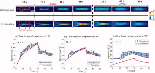
The experimental time profile of the temperature below 45 °C could not be compared with that of the simulation because 45 °C was set as the lower limit of the temperature for the background region with a temperature distribution of less than 45 °C as shown in the profile of 0–5 s in Figure 10(c,d) and 0–7 s in Figure 10(e).

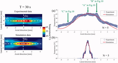
The 1-D spatial temperature profile along the axial and lateral axes of the HIFU focus in the experiments was compared with that of the simulation to evaluate the spatial similarity of the temperature distribution. Figure 11(a,b) compares the 1-D temperature profile along the axial and lateral axes at 30 s between the experiment and the simulation. The positions of ‘A’, ‘B’ and ‘C’ in Figure 10 are indicated by a green arrow in Figure 11(a). As shown in Figure 11(a), the spatial profile around the HIFU focus matched relatively well with that of the simulation. Although the temperature profile along the lateral direction matched well with that of the simulation, there was a temperature difference in the region that was approximately more than 3.0 mm away from the HIFU focus (Figure 11(b)).

Figure 11. Comparison of a one-dimensional (1-D) spatial profile along the (a) axial and (b) lateral axis of the high intensity focused ultrasound (HIFU) focus at 30 s between the experiment and the simulation.

4. Discussion

The color of the lower layer (45–55 °C) started to change before that of the upper layer (55–65 °C) according to the temperature rise at the HIFU focus. These results imply that our new concept for expanding the visible range of temperature rise was effective during and after HIFU exposure.

In order to investigate the accuracy of the temperature rise during and after HIFU exposure, the experimental time profile of the temperature rise was compared with the simulation results. The experimental time profile at and near the HIFU focus matched relatively well with that of the simulation results, although there was a slight difference in the temperature from approximately 10–20 s. Hence, the proposed method could be applied as a tool to investigate the output of the HIFU transducer before treatment. Notwithstanding, the experimental time profile of temperature at ‘C’, which was 3.0 mm in front of the HIFU focus along the axial direction, was much larger than that of the simulation for the entire heating and cooling period.

To discuss the temperature difference between the experiment and simulation at ‘C’, the 1-D experimental spatial profile of the temperature distribution along the axial and lateral axes of the HIFU focus was compared with that of the simulation at 30 s. The experimental spatial profile along the axial direction matched relatively well with that of the simulation at and near the HIFU focus, except for the region that was more than 3.0 mm away from the HIFU focus. However, the spatial profile along the lateral direction nearly completely matched with the simulation.

It was unclear why the lateral temperature profile matched well with that of the simulation compared with the axial profile. One possible explanation is that the physical heterogeneity at the boundary and the difference in attenuation between the two phantoms could have distorted the axial temperature profile.

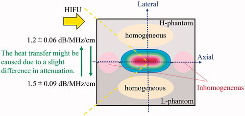
Figure 12 shows a diagram explaining the difference between the experimental and simulation results in the axial temperature profile. The boundary between the H- and L-phantoms was physically inhomogeneous compared to the region of the single material. Moreover, the heat transfer from the H- (or L-) to the L (or H-) phantom might have resulted from a difference in the attenuation between the phantoms. Therefore, these two factors might have induced an unexpected thermal diffusion in the axial direction compared to that in the lateral direction, thereby affecting the axial temperature profile. This speculation requires further investigation for verification and can be achieved by altering the simulation model and experimental parameters, such as acoustic power. However, the main objective of this study was to develop a method enabling users to conveniently assess the output at the HIFU focus before treatment; thus, the proposed method is applicable in clinical practice.

Figure 12. Diagram to explain the difference between the experimental and simulation results in the axial temperature profile.

The experimental spatial profile is shaped like a ‘rectangle wave’, unlike that of the simulation; that is, the temperature rapidly increased from approximately 55 to 60 °C. This is probably because the experimental temperature distribution was produced by flipping the lower or upper layer along the boundary of the phantom, and the 55 °C temperature served as the transition point for the production of temperature distribution using two layers.

In this study, calibration was performed using the relationship between temperature decrease and phantom color change, and the calibration data were applied to the temperature estimation during and after HIFU exposure. The converted temperature in the experiment matched well with that in the simulation around the HIFU focus during the heating and cooling periods. Thus, no hysteresis was visible between the color change and temperature in the proposed phantom, implying that this method can be utilized for measuring the temperature during the heating and cooling periods.

We compared the experimental results with those of the simulation to evaluate the accuracy of the phantom temperature measurement in this study. The use of thermocouples during HIFU experiments was beneficial for validating the thermal and acoustic properties that were used in the simulation. However, measuring 2-D temperature distribution (whole region of the phantom) during HIFU exposure using thermocouples is challenging. In addition, the viscous heating effect of thermocouples could have affected the accuracy of the temperature measurement. Therefore, the measured temperature – converted from the phantom color – was compared with that of the simulation. Moreover, the thermal and acoustic properties that were used in the simulation are relatively reasonable because the measured temperature at and near focus matched well with those of the simulation.

In this study, a new method using a two-layer temperature-sensitive phantom was developed to visualize a range of temperature rise, which was two times wider than the conventional range [22]; nonetheless, discrepancies in the simulation results and challenges warranting improvement exist. A visible temperature range of 20 °C is larger than that of the conventional range, but it should be expanded to more than 40 °C, considering the clinical usage for mimicking the temperature rise in tissues. Furthermore, a more detailed calculation of the thermal dose of tissues [30,31] – a criterion for estimating tissue denaturation – should be performed by measuring a wider range of temperature rise.

5. Conclusions

We developed a new visualization method to measure a wider range of temperature rise during HIFU exposure. The experimental results were comparable to those of the simulation. The total range of the measured temperature rise was two times wider than that of the conventional range, although there is room for improved accuracy. The reason for the difference in the temperature rise in an area far from the HIFU focus along the axial direction warrants further investigation. Nevertheless, the experimental time profile and spatial distribution around the HIFU focus matched relatively well with those of the simulation, and the proposed method can be potentially used in clinical practice to readily check the output of the HIFU transducer prior to treatment. The visible range of temperature can be increased further, and a more detailed calculation of the thermal dose of tissues can be performed by expanding our proposed method using many kinds of MTLC.

Geolocation information

Medical Devices Research Group, Health and Medical Research Institute, National Institute of Advanced Industrial Science and Technology (AIST), 1-2-1 Namiki, Tsukuba, Ibaraki, 305-8564, Japan.

Acknowledgments

The authors would like to express their sincere thanks to Dr. S. Yoshizawa and Dr. S. Umemura of Tohoku University for their cooperation in constructing the experimental setup.

Disclosure statement

No potential conflict of interest was reported by the author(s).

Additional information

Funding

This work was supported by a Grant-in-Aid for Young Scientists [19K20725].

References

- Yu W, Tang L, Lin F, et al. High-intensity focused ultrasound: noninvasive treatment for local unresectable recurrence of osteosarcoma. Surg Oncol. 2015;24(1):9–15.
- Huang Y, Alkins R, Schwartz ML, et al. Opening the blood-brain barrier with MR imaging-guided focused ultrasound: preclinical testing on a trans-human skull porcine model. Radiology. 2017;282(1):123–130.
- Maloney E, Hwang JH. Emerging HIFU applications in cancer therapy. Int J Hyperthermia. 2015;31(3):302–309.
- Takagi R, Jimbo H, Iwasaki R, et al. Feasibility of real-time treatment feedback using novel filter for eliminating therapeutic ultrasound noise with high-speed ultrasonic imaging in ultrasound-guided high-intensity focused ultrasound treatment. Jpn J Appl Phys. 2016;55(7S1):07KC10.
- Takagi R, Goto K, Jimbo H, et al. Elimination of therapeutic ultrasound noise from pre-beamformed RF data in ultrasound imaging for ultrasound-guided high-intensity focused ultrasound treatment. Jpn J Appl Phys. 2015;54(7S1):07HD10.
- Rischmann P, Gelet A, Riche B, et al. Focal high intensity focused ultrasound of unilateral localized prostate cancer: a prospective multicentric hemiablation study of 111 patients. Eur Urol. 2017;71(2):267–273.
- Bass R, Fleshner N, Finelli A, et al. Oncologic and functional outcomes of partial gland ablation with high intensity focused ultrasound for localized prostate cancer. J Urol. 2019;201(1):113–119.
- Peek MC, Ahmed M, Scudder J, et al. High intensity focused ultrasound in the treatment of breast fibroadenomata: results of the HIFU-F trial. Int J Hyperthermia. 2016;32(8):881–888.
- Guan L, Xu G. Damage effect of high-intensity focused ultrasound on breast cancer tissues and their vascularities. World J Surg Oncol. 2016;14(1):153.
- Imai K, Allard M-A, Castro Benitez C, et al. Long-term outcomes of radiofrequency ablation combined with hepatectomy compared with hepatectomy alone for colorectal liver metastases. Br J Surg. 2017;104(5):570–579.
- Huppert P, Wenzel T, Wietholtz H. Transcatheter arterial chemoembolization (TACE) of colorectal cancer liver metastases by Irinotecan-Eluting microspheres in a salvage patient population. Cardiovasc Intervent Radiol. 2014;37(1):154–164.
- Marinova M, Wilhelm-Buchstab T, Strunk H. Advanced pancreatic cancer: high-intensity focused ultrasound (HIFU) and other local ablative therapies. RoFo. 2019;191(3):216–227.
- Marinova M, Rauch M, Mücke M, et al. High-intensity focused ultrasound (HIFU) for pancreatic carcinoma: evaluation of feasibility, reduction of tumour volume and pain intensity. Eur Radiol. 2016;26(11):4047–4056.
- Medvid R, Ruiz A, Komotar RJ, et al. Current applications of MRI-Guided laser interstitial thermal therapy in the treatment of brain neoplasms and epilepsy: a radiologic and neurosurgical overview. Am J Neuroradiol. 2015;36(11):1998–2006.
- Okita K, Ono K, Takagi S, et al. Development of high intensity focused ultrasound simulator for large-scale computing. Int J Numer Meth Fluids. 2011;65(1–3):43–66.
- Narumi R, Matsuki K, Mitarai S, et al. Focus control aided by numerical simulation in heterogeneous media for high-intensity focused ultrasound treatment. Jpn J Appl Phys. 2013;52(7S):07HF01.
- Qiao S, Elbes D, Boubriak O, et al. Delivering focused ultrasound to intervertebral discs using time-reversal. Ultrasound Med Biol. 2019;45(9):2405–2416.
- Hanayama H, Nakamura T, Takagi R, et al. Simulation of optical propagation based on wave optics for phase retrieval in shadowgraph of ultrasonic field. Jpn J Appl Phys. 2017;56(7S1):07JC13.
- Pulkkinen A, Leskinen JJ, Tiihonen A. Ultrasound field characterization using synthetic schlieren tomography. J Acoust Soc Am. 2017;141(6):4600.
- Huang J, Holt RG, Ro C. Experimental validation of a tractable numerical model for focused ultrasound heating in flow-through tissue phantoms. J Acoust Soc Am. 2004;116(4):245.
- Ghanouni P, Pauly KB, Elias WJ, et al. Transcranial MRI-guided focused ultrasound: a review of the technologic and neurologic applications. Am J Roentgenol. 2015;205(1):150–159.
- Iwahashi T, Tang T, Matsui K, et al. Visualization of temperature distribution around focal area and near fields of high intensity focused ultrasound using a 3D measurement system. ABE. 2018;7:1–7.
- Tsujiyama S-I, Miyamori A. Assignment of DSC thermograms of wood and its components. Thermochim Acta. 2000;351(1–2):177–181.
- Healy JJ, de Groot JJ, Kestin J. The theory of the transient hot-wire method for measuring thermal conductivity. Physica. 1976;82(2):340–392.
- Maćkiewicz A, Ratajczak W. Principal components analysis (PCA). Comput Geosci. 1993;19(3):303–342.
- Treeby BE, Wise ES, Kuklis F, et al. Nonlinear ultrasound simulation in an axisymmetric coordinate system using a k-space pseudospectral method. J Acoust Soc Am. 2020;148(4):2288.
- Martin E, Jaros J, Treeby BE. Experimental validation of k-wave: nonlinear wave propagation in layered, absorbing fluid media. IEEE Trans Ultrason Ferroelectr Freq Control. 2020;67(1):81–91.
- Treeby BE, Jaros J, Rendell AP, et al. Modeling nonlinear ultrasound propagation in heterogeneous media with power law absorption using a k-space pseudospectral method. J Acoust Soc Am. 2012;131(6):4324–4336.
- Treeby BE, Cox BT. k-Wave: MATLAB toolbox for the simulation and reconstruction of photoacoustic wave fields. J Biomed Opt. 2010;15(2):021314.
- Sapareto SA, Dewey WC. Thermal dose determination in cancer therapy. Int J Radiat Oncol Biol Phys. 1984;10(6):787–800.
- Andreeva TA, Berkovich AE, Bykov NY, et al. High-intensity focused ultrasound: heating and destruction of biological tissue. Tech Phys. 2020;65(9):1455–1466.