Rapid SAR optimization for hyperthermic oncology: combining multi-goal optimization and time-multiplexed steering for hotspot suppression

Abstract

Purpose

Healthy tissue hotspots are a main limiting factor in administering deep hyperthermia cancer therapy. We propose an optimization scheme that uses time-multiplexed steering (TMPS) among minimally correlated (nearly) Pareto-optimal solutions to suppress hotspots without reducing tumor heating. Furthermore, tumor heating homogeneity is maximized, thus reducing toxicity and avoiding underexposed tumor regions, which in turn may reduce recurrence.

Materials and methods

The novel optimization scheme combines random generation of steering parameters with local optimization to efficiently identify the set of (Pareto-) optimal solutions of conflicting optimization goals. To achieve simultaneous suppression of hotspots, multiple steering parameter configurations with minimally correlated hotspots are selected near the Pareto front and combined in TMPS. The performance of the novel scheme was compared with that of a multi-goal Genetic Algorithm for a range of simulated treatment configurations involving a modular applicator heating a generic tumor situated in the bladder, cervix, or pelvic bone. SAR cumulative histograms in tumor and healthy tissue, as well as hotspot volumes are used as metrics.

Results

Compared to the non-TMPS optimization, the proposed scheme was able to reduce the peak temperature in healthy tissue by 0.2 °C–1.0 °C (a thermal dose reduction by at least 26%) and, importantly, the hotspot volume above 42 °C in healthy tissue by 41%–86%. At the same time, tumor heating homogeneity was maintained or improved.

Conclusions

The extremely rapid optimization (5 s for TMPS part, on a standard PC) permits closed-loop treatment reoptimization during treatment administration, and empowers physicians with a selection of optimal treatment scenarios reflecting different weighting of conflicting treatment goals.

Keywords:

• Treatment optimization
• hyperthermia cancer therapy
• hotspot suppression

1. Introduction

Hyperthermia therapy, i.e., targeted tumor heating to at least 40 °C – preferably above 42–43 °C – for a duration of about one hour, is typically used as an adjuvant to radio- and/or chemotherapy in cancer treatment. In the case of deep seated tumors, selective heating is usually achieved though coherent combination of electromagnetic (EM) energy from multiple radiating elements. However, energy deposition in overlaying tissue structures, as well as field enhancement near interfaces with high dielectric contrast, make it challenging to achieve elevated tumor heating without also introducing hotspots in healthy tissue. Such hotspots can lead to unwanted collateral toxicity or can cause pain, thus limiting the treatment dose tolerable by the patient and the treatment success.

In the context of hyperthermia treatment planning, multiple optimization schemes have been introduced [1–6] to increase selective energy-delivery to the tumor. Furthermore, in deep loco-regional hyperthermia it is very challenging to completely avoid unwanted hotspots, other aspects such as peak temperature in the healthy tissue or the volume of hotspots in the healthy tissue also become relevant. Different quality indicators [7] have been introduced and used as optimization goals. Examples include the ratio between the energy deposition in the tumor and the healthy tissue, the peak temperature in healthy tissue, iso-percentiles of the specific absorption rate (SAR) or the temperature in targeted and non-targeted tissues and thermal dose iso-percentiles. Yet, it was found that the type of optimization goal strongly impacts the optimized treatment parameters and the assessment of the treatment quality [8]. As each quality indicator reflects different, potentially conflicting treatment considerations (e.g., maximal tumor heating, avoidance of underexposed tumor regions, maximization of tumor temperature homogeneity, avoidance of hotspots, optimal energy focusing and efficiency), multi-goal optimization approaches which provide an intuitive way of weighting the different optimization goals transparently to select a suitable compromise are considered a much more desirable approach [9]. For instance, the goal of minimizing the peak SAR in a hotspot, the total hotspot volume, and the tumor temperature homogeneity, all at the same time, while achieving high tumor heating, are likely conflicting goals in the planning and optimization of a patient-specific treatment protocol, which could be weighed against each other. Multi-goal optimization can empower experts by permitting experience- and/or feedback-based interactive weighting of conflicting goals during treatment planning and administration [9], e.g., to manage conflicting hotspots [10].

Optimization approaches that require a large number of successive EM or thermal simulations can quickly become expensive in terms of computational costs, as a high discretization resolution is required to reliably and accurately predict hotspots in the heterogeneous anatomical environment [11].

Time multiplexed steering (TMPS) has been used previously to suppress hotspots in healthy tissue [12–14]. While a set of steering configurations can score similarly high in terms of the chosen SAR or temperature metrics, these configurations can still feature strongly distinct hotspot locations. By combining multiple such configurations in a time-multiplexed manner, a suppression of the time-averaged hotspot intensities can be achieved. Typically, the resulting time-averaged treatment will have slightly inferior SAR metrics (compared to the optimal single configuration), but the exponentially increasing temperature-dependence of biological impact still results in the superiority of the TMPS optimized treatment compared to a non-TMPS optimized treatment. Zastrow et al. [12] studied TMPS of multiple beamforms for microwave hyperthermia on different brain tumors locations, reducing unintended heating of healthy tissue without affecting tumor treatment temperature. For head-and-neck hyperthermia applications, Cappiello et al. [13,14] assessed the potential of TMPS for hotspot suppression. They used an iterative approach, in which identified hotspots of time multiplexed configurations were successively added as additional minimization goals in a multi-goal optimization scheme. Such an approach frequently leads to the occurrence of additional new hotspot locations [13], demanding further optimization rounds and thus it is difficult to ascertain convergence and predict the number of required iterations.

In this study, we developed a SAR-based multi-goal TMPS optimization scheme for hyperthermia treatment that combines multiple iterations of randomly generated treatment parameter configurations (amplitude and phase settings) and local optimizations starting from Pareto-front points to efficiently generate a dense selection of (nearly) pareto-optimal configurations. From a set of such configurations, the ones with minimal hotspot overlap are identified and optimal time weights are computed for TMPS. The high SAR regions, i.e., potential hotspots, are simultaneously suppressed in the TMPS step, thus avoiding the development of new hotspots. The performance of the newly introduced scheme was compared with that of a multi-goal Genetic Algorithm (GA; gamultiobj method from MATLAB v9.3.0 (Mathworks Inc., Natick, MA) [15]; selected for efficiency and convenience reasons) for a range of simulated treatment configurations involving a modular applicator heating a generic tumor situated in the bladder, cervix, or pelvic bone.

2. Methods

2.1. Setup

To assess the potential of the new optimization scheme, the same simulation scenarios were used as in [16] – a study that investigates a modular applicator concept and compares it with traditional ring applications. The setup comprises a detailed anatomical model from the Virtual Population (ViP) [17]. An irregular shaped 39 cm³ tumor was placed in the bladder, cervix, or pelvic bone as heating target for the modular applicator. For the bladder tumor case, simulations were conducted in the Duke ViP anatomical model; for the pelvic bone and cervical tumor cases, the Ella ViP model was used. Five applicator elements were positioned, using the procedure from [16], which selects placements that maximize energy delivery efficiency to the tumor. The positioning of the modular applicator elements for the three tumor cases is shown in Figure 1. Each element features a bow-tie antenna next to an EM-guiding water-bolus, which is in direct contact with the skin (similar to [18,19]). The water bolus is modeled as cuboid that penetrates the body model, but the voxeling properties ensure that the body model always received priority. As a result, the water-bolus is modeled as being in perfect contact with the body, which might be difficult to achieve in clinical practice, however in [18] a similar water bolus arrangement was used in practice with no significant problems being encountered.

Figure 1. Modular applicator module placement for the bladder tumor setup (a); voxelized model of the cervical tumor setup (b); tumor position, element placement, and SAR distribution for the pelvic bone tumor setup (c).

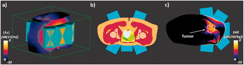
To avoid results dominated by the heating of the non-perfused bladder content and for better heating control, we assume a shrunken, empty bladder and therefore assigned muscle properties to the urine compartment in the anatomical model (as in [16]). Clinical practice varies and while sometimes the bladder is emptied ahead of the treatment, frequently the bladder is filled with saline solution and/or chemotherapeutic agents to improve power deposition and therapeutic efficacy, or it fills up with urine before/during therapy. If it is liquid-filled, convection and the lack of perfusion in the bladder content must be considered [20]. While a filled bladder improves power deposition, it can limit targeting, as the entire bladder wall and surrounding will automatically be heated.

Lower frequency (100 MHz)

In the design study for the modular applicator, frequencies in the range of 200–300 MHz have been found to be optimal. However, most clinically relevant ring applicators operate at a frequency range of 70–100 MHz, resulting in less focal and steerable energy deposition and thus potentially reducing the effectivity of TMPS. Therefore, an additional bladder setup involving the 100 MHz variant of the modular applicator [16] has been studied. The bow-tie antennas and water boli are scaled to account for the longer wave-length and as a result the element placement procedure finds an arrangement with four elements to be optimal.

2.2. EM simulation and SAR evaluation

EM tissue properties were assigned according to the IT’IS Database [21]. The details for the EM simulations are listed in Table 1. Simulations were performed using the finite-difference time-domain solver from Sim4Life v4.4 (ZMT Zurich MedTech AG, Zurich) [22], PML boundary conditions, and an adaptive rectilinear grid. Grid resolution and convergence studies have been performed. For more details, e.g., on the discretization, see [16].

Table 1. Exposure setups for the three tumor cases.

	No. of elements	Freq. [MHz]	Anatomical model
Bladder	5	200	Duke
Cervix	5	300	Ella
Pelvic bone	5	300	Ella

2.3. Thermal simulation

In order to compare the impact of the optimization scheme on the resulting temperature distribution in the tumor and healthy tissue, thermal simulations of the three treatment setups were performed using the transient thermal solver from Sim4Life v4.4 (ZMT Zurich MedTech AG, Zurich). In the first scenario, steering parameters from the multi-goal Genetic Algorithm (GA) were used (individually optimized for each tumor location). In the second scenario, steering parameters from the multi-goal TMPS optimization were used. Thermal simulations were based on the Pennes Bioheat Equation (PBE [23]), which uses a heat sink term proportional to the difference between the local tissue temperature and the arterial blood temperature to account for perfusion cooling. In order to account for the high variability of local perfusion thermoregulation, two temperature-dependent perfusion models – an optimistic (tumor perfusion reduction, strong perfusion increase in healthy tissue) and a more pessimistic model (tumor perfusion increase, reduced increase in healthy tissue) – were used for muscle, skin, fat, and tumor tissue. These two models were based on reported perfusion measurements and models from different studies [24–26] and are identical to those used in [16]. Table 2 summarizes the boundary conditions and the perfusion increase from 37 °C to 45 °C for the two perfusion models. The convective boundary condition to surrounding air assumes a temperature of 25 °C, which differs across hospitals, but has a minor impact on hotspots and tumor heating. The thermal properties of the other tissues are assigned according to the IT’IS Database [21], without temperature dependent thermal properties. For information on the employed spatial discretization, see [16].

Table 2: Thermal simulation settings; boundary conditions (top) and perfusion thermoregulation in muscle, skin, fat, tumor tissue (bottom; based on [24–26]).

Boundary conditions
Interface to	Temperature (°C)	Heat transfer coefficient (W/m^2/K)
Air	25	10
Water bolus	15	140
Perfusion increase from 37° C to 45° C
Tissue	“Optimistic” model	“Pessimistic” model
Muscle	8.8×	6×
Skin	20×	15×
Fat	2×	1.5×
Tumor	0.5×	2×

Other tissues were assigned thermal properties according the IT’IS Database [21], without temperature dependence.

In the simulations of the first scenario, the total applied power was adjusted (iteratively, because of the non-linearity introduced by the temperature-dependent perfusion) such that a peak temperature of 44 ± 0.1 °C was reached during the 60 min treatment. In the simulations of the second scenario, the power was adjusted such that the $T_{50}$ in the tumor, i.e., the temperature exceeded by 50% of the tumor volume (50th isopercentile of the tumor temperature), was identical after an hour of treatment to that of the corresponding first scenario configuration. This scaling ensured that the two scenarios could be directly compared.

For the thermal simulations of multi-goal TMPS-optimized treatment, the heat source SAR distribution was computed as the time weighted average of the SAR distributions from the individual steering configurations (rather than explicitly simulating the switching). This is a reasonable simplification [13], as switching is assumed to occur on a much more rapid scale than the characteristic thermal time-scale, which is in the order of several tens of seconds.

In addition to the $T_{50},$ the $T_{10}$ and $T_{90}$ (10th and 90th isopercentile) were computed and $T_{90}-T_{10}$ was used as tumor temperature homogeneity metric (with a smaller difference indicating better homogeneity).

As hotspot metrics, the volumes of healthy tissue at temperatures above 40, 41, 42, and 43 °C were calculated, respectively. In addition, the peak temperature in healthy tissue ($T_{\mathrm{Max}}$) was extracted. Furthermore, since the thermal impact of heating has a strong, nonlinear dependence on temperature, we also compared the CEM43 thermal dose values [27] at the $T_{\mathrm{Max}}$ location.

2.4. Multi-goal SAR optimization

Multi-goal optimization is valuable when two or more contradicting objectives need to be optimized. In hyperthermic oncology, the primary and frequently conflicting goals are achieving good heating of the tumor on the one hand while avoiding hotspots in healthy tissue on the other. Multi-goal optimization produces a Pareto front of solutions that are all optimal in the sense that one goal cannot be improved on without simultaneously compromising the other goal. Presenting the user, in this case the treating physician, with different optimal solutions, empowering him/her with the ability of weighting conflicting goals based on experience and feedback obtained during the treatment.

In this paper, the following two goals were chosen for minimization:

1. the ratio of average SAR of the healthy tissue and the average SAR of the tumor $\left(\frac{SA{R}_{\mathit{Aver},\mathit{else}}}{SA{R}_{\mathit{Aver},\mathit{tumor}}}\right)$ is a measure for the targeting quality of the energy deposition;

2. the ratio of the peak SAR in healthy tissue and the peak SAR in the tumor $\left(\frac{SA{R}_{\mathit{Max},\mathit{else}}}{SA{R}_{\mathit{Max},\mathit{tumor}}}\right)$ is a measure for the magnitude of hotspots.

Selecting relative quality indicator as a minimization goal is desirable to avoid just favoring low- or high-intensity exposure.

The SAR distribution was calculated after interpolating the electric field (E) to a regular 4 mm rectilinear grid (the original discretization for the E-field computation has an adaptive resolution of 1.0–2.7 mm in the body). SAR averaging was applied (using a sliding cubic volume of 1.2 cm edge length) to mimic thermal diffusion and avoid numerical artifacts. A cube length of 1.2 cm corresponds to 3 × 3 × 3 voxels, which has been found to provide a better correlation with the temperature magnitude and distribution than 2 × 2 × 2 or 4 × 4 × 4 voxels. The outermost 1.2 cm were masked out as the water boli can effectively cool any hotspots near the skin. 1.2 cm is a conservative choice, as water cooling effectively suppresses hotspots up to a depth of around 2 cm [28].

The SAR is computed as: (1) $$\mathit{SAR}=\frac{\sigma {\left|E\right|}^2}{2\rho }$$(1) (2) $${\left|E\right|}^2=\left(\sum _{i=1}^{N_1}{\alpha }_i{E}_i\right){\left(\sum _{i=1}^{N_1}{\alpha }_i{E}_i\right)}^{\mathrm{*}}$$(2) where $N_1$ is the number of antenna elements, $E$ is the coherently combined E-field from all elements, $E_i$ and ${\alpha }_i$ are the E-field distribution and (complex-valued) steering parameter of the ${i\mathrm{th}}^{}$ channel, $\sigma$ is the electrical tissue conductivity, and $\sigma$ is the density.

2.5. Baseline: multi-goal GA optimization

MATLAB’s multi-goal GA gamultiobj method was used to obtain the Pareto front. The population sizes set to 50 and 100 generations were used.

2.6. Multi-goal TMPS optimization

Figure 2 illustrates the multi-goal TMPS optimization pipeline that was used in this study and that was implemented in MATLAB [15]. The pipeline consists of a multi-goal optimization part and a TMPS part. It is assumed that the individual E-field distributions for each antenna element (or channel) are known (from prior EM simulations).

Figure 2. Multi-goal TMPS optimization pipeline.

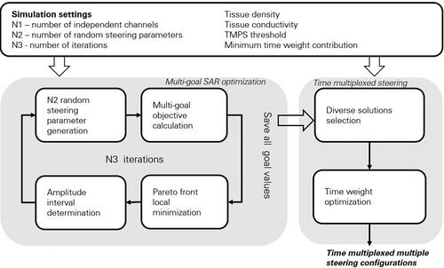
As MATLAB’s gamultiobj method only produces solutions on the Pareto front, while our TMPS approach also requires nearby, but not pareto-optimal, solutions, an additional multigoal optimization process was developed. Another reason for developing our own method is that it requires fewer evaluations and thus provides an additional crucial speed-up.

2.6.1. Multi-goal optimization

The multi-goal optimization process involves multiple iterations. In each iteration, the following steps are performed:

• Stochastic steering parameter generation

  At the beginning of each iteration, $N_2$ random amplitudes and phases are generated. The phases are sampled from a uniform distribution in the range $B_{\mathit{phase}}=[\mathrm{0°}-\mathrm{360°}],$ while the interval for amplitudes selection is updated at every iteration. The initial interval is set as $B_{\mathit{amp}}\mathrm{ }=\mathrm{ }[0.1\mathrm{ }-\mathrm{ }0.6$]. At the beginning of every iteration this range is updated based on the amplitudes of the Pareto front candidates obtained in the previous iteration. The rationale of not having an initial range of $[0-1]$ is that for the studied modular system the elements which show little efficiency in exposing the target region have already been eliminated as part of the element positioning step [16]. The remaining elements should all contribute to the tumor heating while maximally spreading the energy distribution in overlaying tissues. In all investigated scenarios we found that after multiple iterations the amplitude intervals of Pareto-optimal configurations were reduced to below a sixfold range. To maintain flexibility, the amplitude selection interval is updated before each iteration and the local minimization step (see below) also relaxes the interval constraint.

• Multi-goal calculation

  The same EM simulations results, objective functions, grid resolution, and averaging scheme as used for the baseline multi-goal GA optimization are employed.

  $E_i,$ $\rho ,$ $\sigma$ are already known before the optimization. Only the steering parameters ${\alpha }_i$ need to be determined. The most time consuming step of the optimization is the evaluation of Equation (2)(2) $${\left|E\right|}^2=\left(\sum _{i=1}^{N_1}{\alpha }_i{E}_i\right){\left(\sum _{i=1}^{N_1}{\alpha }_i{E}_i\right)}^{\mathrm{*}}$$(2) . Reducing the number of evaluations and the time required for a single evaluation directly impacts the total optimization time. In our implementation, we perform associated large matrix multiplications using hardware acceleration (graphics processing unit-based) provided by the gpuArray() function of MATLAB. For certain functional forms, such as the SAR average ratio employed here, much additional acceleration can be achieved by using precomputed, regionally-averaged interference matrices [29].

  At the end of this step, only the values of the multiple objective functions and the steering parameters are stored.

• Pareto front local minimization

  In this step, unbounded local minimizations are performed, starting from the configurations identified in the multi-goal calculations. In addition to refining the Pareto front, this step is important for the determination of the random sampling amplitude interval of the next iteration.

• Amplitude interval ($B_{\mathit{amp}}$) determination

  The amplitudes of the steering parameters obtained through local minimization are used to determine the new amplitude interval as follows: (3) $$R{b}_i\mathrm{ }=\mathrm{ }\frac{\mathit{max}\left({\alpha }_i\right)}{\mathit{min}\left({\alpha }_i\right)}\mathrm{ }\mathit{for}\mathrm{ }i\mathrm{ }=\mathrm{ }1,\mathrm{ }·N_{\mathit{Pareto}},$$(3) (4) $$B_{\mathit{amp},\mathit{new}}=\mathrm{ }0.1\cdot [1\mathrm{ }–\mathrm{ }\mathit{max}(Rb\left)\right],$$(4)

where $R{b}_i$ is the ratio between the highest and the lowest channel-amplitude of the ${i\mathrm{th}}^{}$ steering parameter configuration on the current Pareto front. The highest ratio determines the new interval range for the random amplitude-sampling step. The unbounded local minimization makes it possible to enlarge the interval, should better configurations be found.

$N_3$ iterations of the above steps are performed. Only the steering parameters and corresponding goal function values are stored. Storage of SAR matrices for every configuration would be costly memory-wise and the few SAR distributions required in the time multiplexing step can be rapidly recomputed.

2.6.2. TMPS optimization

Even when the minimization goal values of two steering configurations are very similar, that does not necessarily mean that the SAR distributions and the hotspot locations are similar. In this section we present the procedure used to identify solutions with similar objective values, but maximally diverse healthy tissue SAR distributions. Then we combine them in TMPS to globally minimizing hotspots.

• Diverse configurations selection

  First, a region of the goal function space with similarly scoring candidate steering parameter configurations is delineated in the vicinity of a user-selected configuration on the Pareto front. The delineation can be performed automatically (using a function that weights and compares the performance of Pareto front solutions compared to the optimally achievable single goal performance) or manually. In the manual scenario, the user interactively selects a region of candidate solutions or shifts the center of an elliptical region along the Pareto front (Figure 4(b)). This permits the user to subjectively weight the relative importance of the goals. Once a group of candidate configurations near the Pareto front have been delineated, a subgroup of configurations that yields an optimal time multiplexed combination needs to be identified. For all candidate configurations, the SAR is recomputed and normalized to an average tumor SAR of 1 W/kg. Next, a mask function is defined, which is non-zero in healthy tissue with SAR above a threshold $\mathit{TMP}{S}_{th}$: (5) $$\mathit{Mask}\left(x,y,z\right)=\mathrm{ }\{\begin{array}{l}1\text{ if }\mathit{SAR}\left(x,y,z\right)>\mathit{TMP}{S}_{th}\\ 0 \text{otherwise} \end{array}$$(5)

Using the $\mathit{Mask}$ for each of the candidate configurations, we can identify steering configurations with minimal hotspot volume overlap. Thirty such minimal-overlap configurations are selected from the candidate configurations.

• Time weight optimization

  Subsequently, the time weight for each minimal-overlap configuration must be chosen, such that hotspots are globally suppressed in healthy tissue. The problem can be formulated as follows: $$\mathit{calculate}\mathrm{ }{w}_i\mathrm{ }in\mathrm{ }SA{R}_{\mathit{TMPS}}\mathrm{ }=\sum _{i=1}^{N_4}{\omega }_{i}SA{R}_i$$ such that the variance of SAR_TMPS is minimized in the masked healthy tissue, where $SA{R}_i$ are the SAR distributions of the minimal-overlap configurations, $SA{R}_{\mathit{TMPS}}$ is the time-averaged TMPS SAR, and ${\omega }_i$ are the time weights.

  Minimizing the variance of $SA{R}_{\mathit{TMPS}}$ is a quadratic programming problem that can be rapidly solved using the covariance matrix.

2.7. Ga and TMPS comparison

For comparison of the SAR distribution of the baseline GA optimization strategy with that of the proposed novel time multiplexed scheme, five steering parameters were selected from the Pareto front obtained using the multi-goal GA optimization as illustrated in Figure 3. Steering parameter configurations 1 and 5 are equivalent to those obtained when individually optimizing for one of the two goals, while the other three correspond to optimal configurations for mixed weighting of both goals. For the assessment of the thermal performance, the central one of these five steering parameters was selected.

Figure 3. Schematic illustration of the Pareto front obtained using multi-goal GA optimization as the baseline optimization. Five steering configurations on the front are selected for SAR comparison with the multi-goal TMPS-optimized exposure. For one of these, a temperature comparison is also performed, based on thermal modeling.

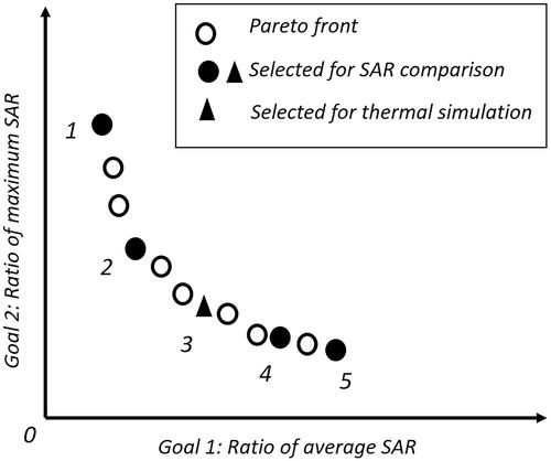
To demonstrate that the five selected treatment configurations indeed correspond to optimized steering parameters that could have been obtained using single-goal optimization with a corresponding weighting of the two goals (the weighting is obtained by fitting a tangent to the Pareto-front through the selected configuration).

The GA-TMPS comparison considers SAR metrics (cumulative SAR histograms in the target tumor and healthy tissue, SAR homogeneity, SAR hotspot magnitude and volume), as well as corresponding thermal metrics.

2.7.1. TMPS optimization settings

Optimization settings were the same for all tumor cases except for the $\mathit{TMP}{S}_{th}$ (see Table 3). As the SAR is normalized to the tumor-averaged SAR, a $\mathit{TMP}{S}_{th}$ of 1.5 (used for the Bladder and Cervix setups) means that only SAR-hotspots in healthy tissue above 1.5 times the tumor average are considered in the TMPS part. In the pelvic bone tumor setup, the SAR-level in healthy tissue was lower than in the other two tumor cases and a value of 0.7 was used instead. The selection of this parameter was performed heuristically, but it could also be included in the optimization procedure. After the time weight optimization, we discarded the configurations with time weights below 4% and only kept the principally contributing configurations to avoid rapidly switching between too many states (it has been observed that 5–10 states typically contribute 95% of the time, and placing the limit at 4% ensures that at most 25 solutions contribute).

Table 3. Multi-goal TMPS optimization settings.

	Bladder	Cervix	Pelvic bone
Number of iterations ($N_3$)		4
Random generated points ($N_2$)	1000 (2000 for the last iteration)
TMPS threshold	1.5	1.5	0.7
Minimal overlap configurations		30
Minimum time weight contribution		4%

3. Results

First, multi-goal GA optimization (two goals) is compared with single-goal optimization using five differently weighted combinations of the two goals, to confirm the equivalent optimality of the solutions. Subsequently, results from different stages of the optimization pipeline in the cervical tumor setup are presented, in order to provide insights into the proposed optimization approach. Next, the multi-goal TMPS optimized SAR is compared against the baseline of the five Pareto-optimal multi-goal GA optimization Pareto front configurations, visualized in the bladder tumor setup as SAR cross-sections, and analyzed for all tumor setups in terms of cumulative histograms. Finally, the performance of the multi-goal TMPS optimization with regard to the induced heating is compared (tumor heating and hotspots) against the GA baseline, using the optimistic and the more pessimistic perfusion thermoregulation models.

The multi-goal TMPS optimization implementation used for this study requires less than 2 min on a personal computer with an Intel i7-4770 processor (3.4 GHz, 4 core) and a graphical processing unit NVIDIA GeForce GTX 760 192-bit (3 GB memory). The TMPS weight optimization requires less than 5 s on a standard PC. EM simulations require 5–10 min per element on a standard workstation with a powerful GPU (NVIDIA Tesla C2070, 6 Gb) and a thermal simulation takes 2–3 min, but the EM simulations only need to be performed once, and can be performed ahead of the time, still enabling near-real-time closed-loop treatment reoptimization during treatment administration.

3.1. Single-goal and multi-goal optimization

Table 4 lists the goal-weighting w that results in a single goal function $G(w)\mathrm{ }=\mathrm{ }(1\mathrm{ }-\mathrm{ }w)·\mathrm{ }G1\mathrm{ }+\mathrm{ }w\mathrm{ }·\mathrm{ }G2$ reproducing the five selected configurations along the Pareto front. The single and multi-goal optimization solutions agree within 4%.

Table 4. Comparison of single- and multi-goal optimization, where the single-goal is a weighted combination of the two goals: $G(w)\mathrm{ }=(1-w)·G_1+w·G_2.$

Comparison of single- and multi-goal GA optimization
Point	Opt.	Goal
In the front	Method	G1	G2	Weight ($\omega$)
1	Multi-goal GA	0.278	4.15
	Single-goal GA	0.289 (4.0%)	4.16 (0.2%)	7.50E-3
2	Multi-goal GA	0.284	3.62
	Single-goal GA	0.289 (1.8%)	3.66 (1.1%)	1.56E-2
3	Multi-goal GA	0.307	3.15
	Single-goal GA	0.306 (-0.3%)	3.17 (0.6%)	6.6E-2
4	Multi-goal GA	0.354	2.90
	Single-goal GA	0.347 (-2.0%)	2.90 (0%)	0.19
5	Multi-goal GA	0.429	2.73
	Single-goal GA	0.443 (3.3%)	2.75 (0.7%)	0.60

The obtained solutions show close goal-performance agreement.

3.2. Multi-goal TMPS optimization pipeline

Figure 4 shows results of the different steps of the multi-goal TMPS optimization for the cervical tumor setup. At the end of the first iteration, the randomly generated points are far from the multi-goal GA optimization generated Pareto front. Local minimization subsequently improves the Pareto front. At the end of the fourth iteration, the best steering configurations closely approximate the multi-goal GA Pareto front. As a next step, a subgroup of 30 steering configuration with minimized hotspot overlap are chosen from an automatically selected candidate region encompassing 100 configurations in the two goal space. For the cervical tumor case, the average pair-wise hotspot overlap volume among these 30 configurations was 47.3 cm³, compared to 80 cm³ among the other 70 steering configurations.

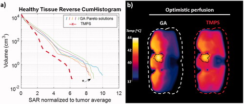
Figure 4. Results of the multi-goal TMPS optimization pipeline for the cervical tumor setup at the end of the first iteration (a) and at the end of the fourth iteration together with the selection region and the Pareto front from the multi-goal GA optimization (b); selection of 30 steering configurations with minimal hotspot overlap (correlation) and optimized time weights for the steering configurations with a contributions greater than 4% (inset) (c); healthy tissue reverse cumulative histograms on a logarithmic and linear scale (d + e) – the histogram corresponding to the GA configuration closest to the center of the TMPS selection region is indicated and the curves are numbered according to Table 4.

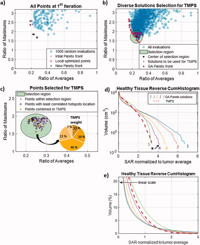
The final optimization step determines the time weights $w_i.$ After discarding configurations that contribute less than 4%, all three tumor cases resulted in less than ten time multiplexed configurations. Figure 4(d) shows the cumulative SAR histograms in healthy tissue for the multi-goal TMPS optimization compared to those of the five configurations from the Pareto front of multi-goal GA optimization.

3.3. SAR cross-sections and cumulative histograms

In all SAR-related graphics, the SAR distributions have been normalized to a 1 W/kg averaged SAR in the tumor as 0 dB. Looking at the SAR cross-sections for the bladder tumor setup, we observe a more homogenous SAR distribution in both tumor and healthy tissue for the multi-goal TMPS optimization (Figure 5). This translates to a more uniformly treated tumor region and to the desired healthy tissue hotspot reduction.

Figure 5. Axial SAR distribution cross-section through the center of the bladder tumor for the five solutions from the Pareto front of the multi-goal GA optimization and for the multi-goal TMPS optimization (inset: magnified tumor region with modified color scale for better contrast). 0 dB corresponds to 1 W/kg. The distribution corresponding to the GA configuration closest to the center of the TMPS selection region is marked with an asterisk. The distributions are numbered as in Table 4 and the numbers are colored as in Figure 4.

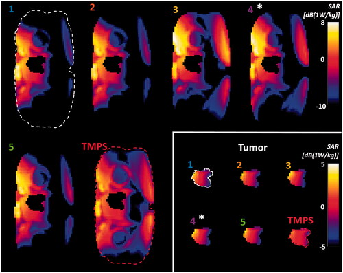
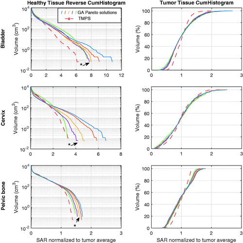
Reverse cumulative histograms were computed that cover the entire treatment volume (Figure 6). We observed a consistent and strong reduction of high SAR exposure regions in healthy tissue for the multi-goal TMPS optimized configuration and an associated important reduction of peak SAR. Additionally, a clear trend to increased tumor exposure homogeneity was apparent. The latter is not an explicit optimization goal, but rather a desirable consequence of averaging between configurations with minimally overlapping hotspots, which is frequently associated with shifting power between applicator elements.

Figure 6. SAR cumulative histograms of healthy tissue (left) and tumor tissue (right) for the five GA Pareto configurations and the TMPS optimized one, for each tumor treatment case. The five GA Pareto configurations are sampled along the entire front and show a shifting compromise between hotspot minimization and tumor exposure maximization. The GA curves are colored as in Figure 4 and the configuration closest to the center of the TMPS selection region is indicated.

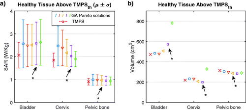
For the healthy tissue above, the threshold used in the TMPS part of the optimization, we calculated the average and standard deviation of the SAR (Figure 7). The results reveal a lower mean and standard deviation for the multi-goal TMPS optimization compared to multi-goal GA optimization, and thus a lower risk of hotspots.

Figure 7. Mean and standard deviation of the SAR in the volume of healthy tissue above the TMPS threshold (0.7 W/kg for pelvic bone, 1.5 W/kg for bladder and cervix) (left), volume of the healthy tissue above the defined threshold SAR (right). The GAs are colored as in Figure 4 and the configuration closest to the center of the TMPS selection region is indicated with an asterisk.

We also quantified the difference in tumor SAR coverage $SA{R}_{10}-SA{R}_{90}$ as a measure of SAR homogeneity in the tumor ($SA{R}_x$ is the SAR value exceeded by x% of tumor volume). The tumor SAR distributions for the GA configurations and the TMPS optimization are provided in Table 5. Results show that the multi-goal TMPS optimization improves SAR homogeneity in the tumor by at least 20%.

Table 5. Quantitative SAR distribution comparison for the GA configurations and the TMPS optimization, for all three tumor cases.

SAR distribution quantification
		Tumor tissue		Healthy tissue
	Opt.	SAR10–SAR90	Change in	SARhotspot (mean)	Change in	Hotspot volume	Change in
	Method	[W/kg]	[%]	[W/kg]	[%]	[cm^3]	[%]
Bladder	GA (range)	[0.97–1.13]		[2.5–2.6]		[478 − 781]
	TMPS	0.6	[−38 to −47]; −38	2.1	[−16 to −19]; −18	472	[−1 to −40]; −17
Cervix	GA (range)	[1.27–1.39]		[1.9–2.5]		[199–328]
	TMPS	1.01	[−20 to −27]; −20	1.8	[−5 to −28]; −15	218	[+10 to −33]; 10
Pelvic bone	GA (range)	[0.8–0.97]		[0.93 − 0.99]		[284–304]
	TMPS	0.59	[−26 to −39]; −33	0.9	[−3 to −9]; −7	314	[+11 to +3]; 10

For tumor tissue $SA{R}_{10}-SA{R}_{90}$ is used as a measure of SAR homogeneity. For healthy tissue, volume of the tissue above $\mathit{TMP}{S}_{\mathrm{t}h}$ and mean SAR value of these volumes are compared (see also Figure 7). The change ranges refer to the five GA configurations, and the change relative to the GA configuration closest to the center of the TMPS selection region is reported separately.

3.4. Thermal simulation results

As the clinically relevant quantity for a successful therapy is the temperature distribution, the performance of the multi-goal TMPS optimized treatments is also compared to one of the multi-goal GA Pareto configurations (the one at the center of the Pareto front, as a compromise between the two objectives – see Figure 3). We were able to show that for the selected GA configuration each tumor was representative of the best steering configurations in terms of thermal simulation results. For the bladder tumor setup, the temperature distribution cross-sections and the cumulative histograms are shown in Figure 8.

Figure 8. Temperature simulation result for the bladder tumor setup, comparing a selected GA Pareto configuration with the TMPS optimized one, using an optimistic and a more pessimistic perfusion thermoregulation model. Axial temperature distribution cross-section through the tumor (a), corresponding temperature cumulative histograms for the healthy tissue (b), and tumor region (c).

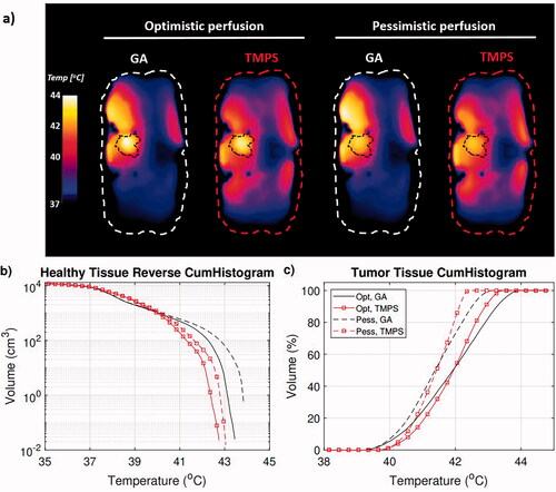
Quantification of the temperature distributions for all three tumor cases can be found in Tables 6 and 7. In all cases, the peak temperature in healthy tissue was lower for the multi-goal TMPS optimization. Accordingly, the volume of healthy tissue above 41 °C and 42 °C is reduced by up to 86%, and the volume above 43 °C up to 100%. In terms of impact (thermal dose), the peak CEM43 exposure of healthy tissue is reduced by at least 26%. The $T_{10}-T_{90}$ metric shows a tumor heating homogeneity improvement by over half a degree for the bladder and pelvic tumor setups, but no improvement was seen for the cervical tumor case, in line with the tumor SAR histograms in Figure 6. Multi-goal TMPS optimization tend to require slightly more power (up to 5%) to achieve the same tumor $T_{50}$ value, indicating that the hotspot reduction is associated with a small reduction of the tumor heating selectivity.

Table 6. Metrics of the temperature distributions obtained with the multi-goal GA optimized and the multi-goal TMPS optimized exposures, for all three tumor cases and for the 100 MHz bladder tumor case (“Optimistic” perfusion thermoregulation model).

Temperature distribution quantification – “Optimistic” perfusion model
			Tumor tissue		Healthy tissue
		Power	T50	T10 –T90	Volume above				TMax	CEM43Max
					40 °C	41 °C	42 °C	43 °C
	Opt. method	[W]	[°C]	[°C]	[cm^3]	[cm^3]	[cm^3]	[cm^3]	[°C]	[min]
	GA	120	41.9	3.0	958	465	140	5	43.5	83
	TMPS	120	41.9	2.3 (−0.7)	987 (+3%)	190 (−59%)	20 (−86%)	0 (−100%)	42.7 (−0.8)	51 (−39%)
Cervix	GA	100	42.3	2.5	1080	345	71	6	44.1	105
	TMPS	105	42.3	2.5 (0)	1117 (+3%)	309 (−10%)	42 (−41%)	2 (−67%)	43.5 (−0.6)	69 (−34%)
Pelvic	GA	34	42.1	2.6	305	44	0.8	0	42.5	19
bone	TMPS	35	42.1	2.1 (−0.5)	294 (-4%)	23 (−48%)	0.15 (−81%)	0	42.3 (−0.2)	14 (−26%)
Bladder	GA	224	41.6	2.7	2138	809	111	2	44.0	104
100 MHz	TMPS	202	41.6	1.4 [−1.3]	2575 (+20%)	333 (−59%)	0.5 (−99.5%)	0 (−100%)	42.4 (−1.6)	23 (−78%)

Table 7. Metrics of the temperature distributions obtained with the multi-goal GA optimized and the multi-goal TMPS optimized exposures, for all three tumor cases and for the 100 MHz bladder tumor case (“Pessimistic” perfusion thermoregulation model).

Temperature distribution quantification – “Pessimistic” perfusion model
			Tumor tissue		Healthy tissue
		Power	T50	T10 –T90	Volume above				TMax	CEM43Max
					40^oC	41^oC	42^oC	43^oC
	Opt. method	[W]	[°C]	[°C]	[cm^3]	[cm^3]	[cm^3]	[cm^3]	[°C]	[min]
Bladder	GA	118	41.4	2.3	1065	568	262	65	44.0	104
	TMPS	118	41.4	1.6 (−0.7)	1164 (+9%)	317 (−44%)	50 (−81%)	0 (−100%)	43.0 (−1.0)	61 (−41%)
Cervix	GA	94	41.3	1.8	1135	413	78	8	44.0	101
	TMPS	98	41.3	1.8 (0)	1160 (+2%)	358 (−13%)	39 (−50%)	2 (−75%)	43.5 (−0.5)	68 (−33%)
Pelvic	GA	48	42.5	2.1	643	292	53	0.2	43.2	55
bone	TMPS	49	42.5	1.6 (−0.5)	654 (+2%)	266 (−9%)	14 (−74%)	0 (−100%)	42.7 (−0.5)	31 (−44%)
Bladder	GA	212	41.1	2.1	2218	1065	271	5	44.1	110
100 MHz	TMPS	196	41.1	0.7 (−1.4)	3153 (+42%)	634 (−40%)	4 (−98.5%)	0 (−100%)	42.6 (−1.5)	26.3 (−76%)

3.5. Lower frequency (100 MHz)

The metrics for the 100 MHz bladder tumor setup can be found in Tables 6 and 7, while distributions and histograms can be seen in Figure 9. Despite the larger focus and the reduced targeting/steering capability, TMPS provides an important benefit. The reason is probably that the lower frequency results in deeper penetration, such that more elements can provide a similar contribution to tumor heating and thus the diversity of available solutions for multiplexing increases, which in turn reduces the time-averaged exposure of healthy tissue.

Figure 9. Treatment of bladder tumor with 100 MHz 4-element applicator: (a) healthy tissue SAR histograms of five Pareto-optimal solutions from GA optimization and from TMPS optimization (the GAs are colored as in Figure 4 and the configuration closest to the center of the TMPS selection region is indicated); (b) axial temperature distribution cross-sections through the tumor (optimistic perfusion model).

4. Discussion

Ideal and worst-case TMPS performance relative to GA optimized single configuration. In this study, we compare a new multi-goal TMPS optimization approach with a multi-goal GA optimization scheme, demonstrating the superiority of the achievable SAR and temperature distributions in terms of hotspot reduction and tumor heating homogeneity. In an ideal scenario, TMPS can identify multiple (n) configurations that perform similarly with regard to the optimization goals, but have no hotspot overlap. With equal time-weights, that would result in a (time-) averaged hotspot SAR that is n-times lower than for a single configuration, while the (time- and space-) averaged tumor SAR is maintained. (Similar considerations also apply for underexposed tumor regions.) As a single steering parameter configuration constitutes a border-case of the TMPS configuration space, it is inherently guaranteed (within the limits of global optimum identification) that the TMPS optimized treatment cannot be inferior. The same argument holds with regard to multi-goal versus single objective optimization. Adding hotspot suppression as additional objective means accepting a reduction of tumor targeting efficiency, for the sake of avoiding hotspots in healthy tissue. Because $SA{R}_{\mathit{TMPS}}\mathrm{ }={\sum }_{i=1}^{N_4}{\omega }_{i}SA{R}_i,$ the first optimization goal $R1=\left(\frac{SA{R}_{\mathit{Aver},\mathit{else}}}{SA{R}_{\mathit{Aver},\mathit{tumor}}}\right)$ becomes: (6) $$R{1}_{\mathit{TMPS}}=\frac{{\sum }_{i=1}^{N_4}{\omega }_{i}SA{R}_{\mathit{Aver},\mathit{else},i}}{{\sum }_{i=1}^{N_4}{\omega }_{i}SA{R}_{\mathit{Aver},\mathit{tumor},i}}=\frac{{\sum }_{i=1}^{N_4}{\omega }_{i}SA{R}_{\mathit{Aver},\mathit{tumor},i}R{1}_i}{{\sum }_{i=1}^{N_4}{\omega }_{i}SA{R}_{\mathit{Aver},\mathit{tumor},i}}=\sum _{i=1}^{N_4}{\omega }_i^{\mathrm{*}}R{1}_i,$$(6) which can be interpreted as a weighted average between the ratios $R{1}_i$ of the contributing configuration with weights ${\omega }_i^{\mathrm{*}}=\frac{{\omega }_{i}SA{R}_{\mathit{Aver},\mathit{tumor}.\mathrm{ }i}}{{\sum }_{j=1}^{N_4}{\omega }_{j}SA{R}_{\mathit{Aver},\mathit{tumor},j}}.$ As such, any TMPS SAR distribution is guaranteed to perform equally well with regard to the first goal as the contributing single configurations (which are selected from a region of similarly performing configurations). Therefore, TMPS can be seen as a strategy to generate exposures that shift the healthy tumor exposure away from hot-spot regions and toward cooler regions – it cannot improve the first goal ($R1$), but it can maintain a similar performance while optimizing the second goal. This is apparent in Figures 4 and 6, where the TMPS strategy produces (i) peak SAR values (tumor-average-normalized) in healthy tissue that are equal or superior to the best GA configuration (GA5), while (ii) reducing the healthy tissue exposure in hot-spots (see Figure 7) and elsewhere (the TMPS curves are below the GA5 curve), and (iii) maintaining the $R1$ performance of the GA3 or GA4 configuration – around which the TMPS-contributing configurations have been selected – by shifting energy from the high-SAR to the low-SAR regions (as evident in the cumulative histogram curve, which is below the GA3/GA4 curve at high SAR values, but above it at low SAR values).

It should be pointed out that in this study the hotspot reduction scheme was tested on a modular applicator design [16] – a design that already eliminates applicator elements with a poor targeting efficiency (and thus, a high relative heating of non-target tissues). It is thus expected, that the presented multi-goal TMPS optimization approach would prove to be even more beneficial when applied to a rigid ring applicator.

SAR versus temperature optimization: There is a fundamental debate in the hyperthermia treatment planning community, whether SAR-based optimization (less uncertainty about dielectric parameters and dosimetric quantities) or temperature-based optimization (large inter- and intra-subject variability of relevant tissue properties, such as perfusion, resulting less reliable predictions; but more directly relevant to the treatment safety and efficacy) is preferable (e.g., [30,31]). In this study, SAR-based optimization was used, but the quantitative analysis was carried out in terms of SAR and temperature. To account for the important perfusion thermoregulation uncertainty, two models were considered, as in [16,32]. However, the presented approach can be readily generalized to temperature-based optimization. Applying the transient heating estimation approach from [33], which is well suited to large exposure volumes and accounts for local thermoregulation and body-core temperature increase, this could even be achieved without large computational overhead.

Scaling: For the comparison of the TMPS- and GA-optimized therapy plans, the SAR scaling has been adjusted to produce matching tumor temperature medians. Clinically, it can be desirable to instead scale them such that hot-spots reach a similar magnitude (at the threshold of patient tolerance or tissue damage). From the results in Tables 6 and 7, as well as Figure 8, it is apparent that this would result in a tumor temperature increase of about 0.5–1.5 °C. This would particularly benefit the Cervix scenario, where tumor exposure is not improved by TMPS with the current scaling, but could be increased by about 0.5 °C when applying hot-spot-limited scaling.

Optimization performance and closed-loop treatment administration: The total computation time depends on the number of voxels and the number of antenna elements. The most time consuming part is the SAR computation for the random generated steering parameter configurations. Additional optimization objectives can be added – e.g., adding a third objective would result in a 3D goal-value space with a 2D-parameterizable Pareto front. Covering that front with sufficient density could demand more configuration sampling (at least when the goals are poorly correlated) – even though the steering parameter space size remains unchanged – potentially increasing the computational effort. Increasing the number of applicator elements will likely result in a significant increase in computational effort. The presented method is easily parallelizable. The TMPS part of the optimization is so fast (less than 5 s in our implementation), that reoptimization based on a precomputed Pareto front is possible during treatment administration. This means that it is possible to react to online feedback (from implanted sensors, other monitoring devices, or the patient).

Implementation: The combination of unbounded local optimization with random configuration generation not only allows to further improve optimization goals but also reduces the risk of missing optimal configurations outside the initial amplitude sampling interval. The threshold for identifying diverse solutions and optimizing the time weights was fixed and identical for all tissues in this study. However, a variable threshold based on tissue properties, such as heat sensitivity (to suppress exposure of sensitive tissues) or heatability, could be used.

Clinical realization: In view of the thermal time constant of living tissue, which is in the order of several tens of seconds, the technical difficulty of supporting sufficiently rapid switching between steering parameters is small. However, existing commercial systems do not currently provide such an interface and would therefore need to be modified.

Generalization: A similar approach could be valuable beyond hyperthermia treatment optimization, e.g., for radiotherapy treatment optimization.

Limitations: The principal limitations of this study are the lack of experimental validation and the small number of investigated cases (three tumor location setups – all of them in the abdominal region – and one modular applicator concept). Furthermore, there is a high degree of variability and uncertainty associated with perfusion. The two studied perfusion models are based on [24–26] and were chosen to match [16], but are likely to not reflect the full range. A small modeling study revealed that in the modeled conditions (strong bolus cooling under the applicator elements) the skin thermoregulation model only affects the outermost 1–2 cm by more than 0.1 °C and thus does not impact the hot-spots, which are situated deeper. Lower fat and muscle perfusion increases with temperature would result in more pronounced hot-spots and are expected to amplify the differences between TMPS and non-TMPS strategies (in closer accordance to the SAR metrics).

5. Conclusions

In this study we proposed a novel hyperthermia therapy optimization scheme, which combines multi-goal SAR optimization with TMPS to simultaneously reduce all hotspots in healthy tissue without introducing new ones by combining minimally correlated configurations. Investigations involving simulated treatments of various tumor configurations showed that the proposed optimization scheme could achieve a reduction of the peak temperature in healthy tissue (by 0.2–1.0 °C, corresponding to a toxicity reduction by at least 26% in terms of thermal dose) and an important reduction of the healthy tissue hotspot volume above 42 °C (by 41–86%), while maintaining or improving tumor heating homogeneity (up to 0.7 °C reduction of $T_{10}-T_{90}$). The currently employed SAR-based tumor exposure and hotspot ratio objective functions could readily be replaced or complemented by other (e.g., temperature-based) objectives. TMPS reoptimization takes less than 5 s, which permits feedback-based (closed-loop) reoptimization during treatment administration. Furthermore, the achieved speed permits clinician to interactively weight conflicting objectives and to select from different visualized optimal solutions. Instead of reducing toxicity by suppressing hotspots, it would also be possible to apply the optimized TMPS configuration with increased power, such that the hotspot intensity remains at the level of an optimized single configuration treatment, but the tumor heating and therapeutic efficacy is increased.

Acknowledgements

We gratefully acknowledge funding by the University of Zurich and the IT'IS Foundation and we thank Dr. Sabine Regel (sr-scientific.com) for the various inputs and thorough review of the manuscript.

Disclosure statement

No potential conflict of interest was reported by the author(s).

Additional information

Funding

The author(s) reported there is no funding associated with the work featured in this article.

References

- Cappiello G, McGinley B, Elahi MA, et al. Differential evolution optimization of the SAR distribution for head and neck hyperthermia. IEEE Trans Biomed Eng. 2017;64(8):758–1885.
- Bardati F, Tognolatti P. Hyperthermia phased arrays pre-treatment evaluation. Int J Hyperthermia. 2016;32(8):911–922.
- Cheng K-S, Stakhursky V, Craciunescu OI, et al. Fast temperature optimization of multi-source hyperthermia applicators with reduced-order modeling of 'virtual sources'. Phys Med Biol. 2008;53(6):1619–1635.
- Iero DAM, Isernia T, Morabito AF, et al. Optimal constrained field focusing for hyperthermia cancer therapy: a feasibility assessment on realistic phantoms. PIER. 2010;102:125–141.
- Köhler T, Maass P, Wust P, et al. A fast algorithm to find optimal controls of multiantenna applicators in regional hyperthermia. Phys Med Biol. 2001;46(9):2503–2514.
- Nguyen PT, Abbosh A, Crozier S. Three-dimensional microwave hyperthermia for breast cancer treatment in a realistic environment using particle swarm optimization. IEEE Trans Biomed Eng. 2017;64(6):1335–1344.
- Canters RAM, Wust P, Bakker JF, et al. A literature survey on indicators for characterisation and optimisation of SAR distributions in deep hyperthermia, a plea for standardisation. Int J Hyperthermia. 2009;25(7):593–608.
- Seebass M, Beck R, Gellermann J, et al. Electromagnetic phased arrays for regional hyperthermia: optimal frequency and antenna arrangement. Int J Hyperthermia. 2001;17(4):321–336.
- Neufeld E, Kyriacou A, Paulides M, et al. Enabling operator interaction in hyperthermia treatment planning using pareto optimization. In Proceedings of the 2010 Society for Thermal Medicine Conference, Clearwater, FL, USA, April 23–26, 2010.
- Kyriakou A, Neufeld E, Fuetterer M, et al. Multi-objective optimization with automatic risk region detection for interactive hyperthermia treatment planning and adjustment. In 30th Annual Meeting of the Society for Thermal Medicine (STM 2013), Palm Beach, Aruba, April 17–21, 2013.
- Kok HP, Haaren PMAV, de Kamer JBV, et al. High-resolution temperature-based optimization for hyperthermia treatment planning. Phys Med Biol. 2005;50(13):3127–3141.
- Zastrow E, Hagness SC, Veen BDV, et al. Time-multiplexed beamforming for noninvasive microwave hyperthermia treatment. IEEE Trans Biomed Eng. 2011;58(6):1574–1584.
- Cappiello G, Drizdal T, Mc Ginley B, et al. The potential of time-multiplexed steering in phased array microwave hyperthermia for head and neck cancer treatment. Phys Med Biol. 2018;63(13):135023.
- Cappiello G, Paulides MM, Drizdal T, et al. Robustness of time-multiplexed hyperthermia to temperature dependent thermal tissue properties. IEEE J Electromagn RF Microw Med Biol. 2020;4(2):126–132.
- MATLAB version 9.3.0.713579 (R2017b). Natick, MA: The Mathworks, Inc., 2017.
- Poni R. 2021. Precision hyperthermia: the role of modular radiofrequency applicators, electrical impedance tomography and online optimization [doctoral dissertation]. ETH Zurich; 2021.
- Gosselin M-C, Neufeld E, Moser H, et al. Development of a new generation of high-resolution anatomical models for medical device evaluation: the virtual population 3.0. Phys Med Biol. 2014;59(18):5287–5303.
- Dressel S, Gosselin M-C, Capstick MH, et al. Novel hyperthermia applicator system allows adaptive treatment planning: preliminary clinical results in tumour-bearing animals. Vet Comp Oncol. 2018;16(2):202–213.
- Capstick MH, Gosselin M-C, Neufeld E, et al. Novel applicator for local RF hyperthermia treatment using improved excitation control. In 2014 XXXIth URSI General Assembly and Scientific Symposium (URSI GASS), 2014, pp. 1–4.
- Schooneveldt G, Kok HP, Bakker A, et al. Clinical validation of a novel thermophysical bladder model designed to improve the accuracy of hyperthermia treatment planning in the pelvic region. Int J Hyperthermia. 2018;35(1):383–397.
- Hasgall P, Neufeld E, Gosselin MC, et al. IT’IS Database for thermal and electromagnetic parameters of biological tissues. Version 4.0, May 15, 2018. VIP21000-04-0. Available from: www.itis.swiss/database 2018.
- Sim4Life version 4.4. Zurich, Switzerland: ZMT ZurichMedTech, 2019.
- Pennes HH. Analysis of tissue and arterial blood temperatures in the resting human forearm. J Appl Physiol. 1948;1(2):93–122.
- Rossmann C, Haemmerich D. Review of temperature dependence of thermal properties, dielectric properties, and perfusion of biological tissues at hyperthermic and ablation temperatures. Crit Rev Biomed Eng. 2014;42(6):467–492.
- Song CW, Chelstrom LM, Aumschild DJ. Changes in human skin blood flow by hyperthermia. Int J Radiat Oncol Biol Phys. 1990;18(4):903–907.
- Lang J, Erdmann B, Seebass M. Impact of nonlinear heat transfer on temperature control in regional hyperthermia. IEEE Trans Biomed Eng. 1999;46(9):1129–1138.
- Sapareto SA, Dewey WC. Thermal dose determination in cancer therapy. Int J Radiat Oncol Biol Phys. 1984;10(6):787–800.
- Van der Gaag M, De Bruijne M, Samaras T, et al. Development of a guideline for the water bolus temperature in superficial hyperthermia. Int J Hyperthermia. 2006;22(8):637–656.
- Neufeld E. High resolution hyperthermia treatment planning. Vol. 52. Switzerland: ETH Zurich; 2008.
- Canters RAM, Paulides MM, Franckena M, et al. Benefit of replacing the sigma-60 by the Sigma-Eye applicator. A Monte Carlo-based uncertainty analysis. Strahlenther Onkol. 2013;189(1):74–80.
- De Greef M, Kok H, Correia D, et al. Optimization in hyperthermia treatment planning: the impact of tissue perfusion uncertainty. Med Phys. 2010;37(9):4540–4550.
- Drizdal T, Paulides MM, van Holthe N, et al. Hyperthermia treatment planning guided applicator selection for sub-superficial head and neck tumors heating. Int J Hyperthermia. 2018;34(6):704–713.
- Neufeld E, Fuetterer M, Murbach M, et al. Rapid method for thermal dose-based safety supervision during MR scans. Bioelectromagnetics. 2015;36(5):398–407.