Validating a simulation model for laser-induced thermotherapy using MR thermometry

Abstract

Objectives

We want to investigate whether temperature measurements obtained from MR thermometry are accurate and reliable enough to aid the development and validation of simulation models for Laser-induced interstitial thermotherapy (LITT).

Methods

Laser-induced interstitial thermotherapy (LITT) is applied to ex-vivo porcine livers. An artificial blood vessel is used to study the cooling effect of large blood vessels in proximity to the ablation zone. The experimental setting is simulated using a model based on partial differential equations (PDEs) for temperature, radiation, and tissue damage. The simulated temperature distributions are compared to temperature data obtained from MR thermometry.

Results

The overall agreement between measurement and simulation is good for two of our four test cases, while for the remaining cases drift problems with the thermometry data have been an issue. At higher temperatures local deviations between simulation and measurement occur in close proximity to the laser applicator and the vessel. This suggests that certain aspects of the model may need some refinement.

Conclusion

Thermometry data is well-suited for aiding the development of simulations models since it shows where refinements are necessary and enables the validation of such models.

Keywords:

• LITT
• MR thermometry
• modeling
• simulation
• experimental validation

1. Introduction

Laser-induced interstitial thermotherapy (LITT) is a minimally invasive procedure for the local thermal treatment of cancer, which is in practice often used to treat tumors in the liver. For this purpose, a special laser applicator is inserted into the tissue close to the tumor. Laser power is applied directly through the applicator and the tissue around the applicator including the tumor is heated up until coagulative effects cause the destruction of the tumor cells.

One of the main issues of LITT is the planning of the treatment, where the practitioner tries to ensure that all of the tumor cells are being destroyed, while healthy tissue should not be damaged if possible. To aid the practitioners, we consider the simulation of LITT and compare our results with measurements from ex-vivo experiments. Particularly, our focus lies on the influence of blood vessels which are known to have a large influence on the treatment as they act as heat sinks (see e.g. [1]).

Models for simulating LITT have been studied for a long time, e.g. in [2–5]. The main effects which have to be considered in such a model are the propagation of radiation and temperature in the tissue, which are typically modeled by systems of partial differential equations (PDEs). Since the radiation is absorbed by the tissue, it is modeled as a source term for the temperature equation. The local optical and thermal properties of the tissue change once coagulation takes place [6] which e.g. increases the absorption rate. Moreover, even the perfusion properties of the tissue are known to change with increasing temperatures [7].

Two problems arise when dealing with simulations for LITT: First, not all parameters of the model are precisely known or easily measurable and, second, validating the simulation results is no simple task due to the complexity of measuring the temperature and tissue damage during the treatment. In our previous study [5], we used a single temperature probe in order to validate the simulation results. However, comparing the temperatures at a single position is not sufficient to validate the simulation and is of course not possible during real treatments. In this paper, we investigate whether thermometry data obtained from MR imaging can be used to validate the simulation results and possibly even help to identify missing parameters. Thermometry uses MR images to derive local temperature measurements. Hence we can not only compare the results of the simulation at a single point, but at the entire image plane of the MR. In particular, we investigate whether the accuracy and resolution of the thermometry measurements are sufficient to validate the simulation results and whether this information can be used to identify certain missing parameters for the model.

For this study, four ablation experiments with ex-vivo pig livers were carried out. MR imaging was used throughout all experiments to derive thermometry measurements. Additionally, a small tube, acting as an artificial blood vessel, was placed into each of the samples. Water was pumped through the artificial vessel to emulate the cooling effect of blood vessels in the tissue which act as heat sinks and influence the treatment. The same settings were simulated with our computer model and the temperatures obtained from thermometry and simulation were compared in the two-dimensional imaging plane.

2. Materials and methods

2.1. Experimental setup

Magnetic resonance-guided laser ablation was applied to four porcine liver samples. The liver was obtained from a slaughterhouse and used approximately 6 h later for the experiments. For the LITT procedure a ND:YAG laser (MY 30, Martin Medizin-Technik, Tuttlingen, Germany) with a wavelength of 1064 nm and a laser power ${\widehat{q}}_{\text{app}}$ of 20 W was used. A laser applicator (Power-Laser-Set; Somatex® Medical Technologies, Teltow, Germany) was inserted into the middle of the liver sample. An optical fiber with a diffuse emission window of 30 mm at the tip delivered the laser radiation into the applicator (Somatex^® Medical Technologies, Teltow, Germany). The diffuser tip generates a symmetrical ellipsoidal heating pattern whose longitudinal axis is aligned with the applicator orientation. The applicator is transparent for the laser radiation and additionally equipped with an internal cooling water circulation system which is used to cool the surface of the applicator and the surrounding tissue. This is done to prevent overheating and thus carbonization of the tissue as well as damage to the applicator and the optical fiber. The temperature $T_{\text{cool}}$ of the cooling water was 20.0 °C.

To emulate blood flow in a vessel in the ablation area, a plastic tube with a diameter of 4 mm was positioned in the liver perpendicular to the applicator shaft (Figures 1 and 2). To position the tube, the liver was pierced with a needle (diameter of 3 mm) so that the tube could be advanced immediately. This was image-guided after positioning the laser applicator in the liver. The distances between the laser applicator and the tubing were 6, 9, 8, and 8 mm in the four liver samples. A roller pump (Dornier Medizintechnik, Wessling, Germany) was used to pass water through the artificial vessel at a flow rate of 60 ml/min. The temperature $T_{\text{vessel}}$ of the water was 20.5 °C.

Figure 1. MR imaging of the experimental setup in axial (a) and coronary (b) orientation. MR images show the liver in the center (1), the agarose gel phantoms in the periphery (2), the laser applicator (3), the plastic tube (4) passing through the liver (partial representation of the plastic tube in a), and bloodless vessels (5). A schematic in axial orientation with the position of the MR slice is shown in (c). The artificial vessel is positioned at right angles to the applicator and the MR imaging plane.

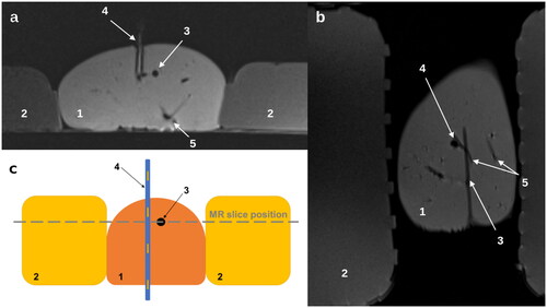
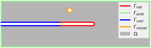
Figure 2. Sketch of the computational domain Ω and the boundary decomposition: radiating surface of the applicator ${\Gamma }_{\text{rad}},$ cooled surface of the applicator ${\Gamma }_{\text{cool}},$ surface of the artificial blood vessel ${\Gamma }_{\text{vessel}},$ and ambient surface of the liver ${\Gamma }_{\text{amb}}.$

The positions in the liver were controlled by MR imaging using the 1.5 T scanner Magnetom Aera (Siemens Healthineers, Erlangen, Germany, Gradient strength = 45 mT/m @ 200 T/m/s, number of channels = 64, coils used: CP Spine Array Coil, Body-18) utilizing a turbo spin echo sequence in coronal and transversal orientation (TR = 700 ms, TE = 12 ms, FOV = 220 × 220 mm,² matrix = 256 × 256). During ablation, a segmented echo planar imaging (seg-EPI) sequence was used for MR thermometry based on the proton resonance frequency shift (PRF) method (TR = 50 ms, TE = 13 ms, flip angle = 12, FOV = 220 × 220 mm,² matrix = 128 × 128, EPI factor = 1, Segments = 3, Echo spacing = 16 ms, one slice in coronal orientation, TA = 2 s).

The PRF method uses the generated image data of the phase shift to calculate a temperature. The method is described in detail in our previous studies [8–10]. The temperature sensitive coefficient α of −0.01 ppm/°C was used to calculate the temperature, which was taken from the work of [10,11]. As described by [12–15], an additional region of interest (ROI) in the phantom (which was not involved by the heating) controlled the B0 field and was used to correct the temperature calculation. Fluoroscopic MR-based thermometry was performed one minute before ablation and for 30 min during ablation at 4-s intervals. Since a homogeneous magnetic field in the object is essential for the PRF method, two agarose gel phantoms were positioned along the liver sample (Figure 1) to optimize the adjustments of the MR system (shimming). The homogeneous phantoms expand the object (liver) for the MR system and thus provide more MR signal to optimize automatic adjustments while reducing susceptibility differences in the peripheral area of the liver. The gel phantoms with an object size of 220 × 90 × 35 mm consisted of saline solution (NaCl content: 0.9%) and 3% agarose. The initial temperatures $T_{\text{init}}$ of the liver samples and phantoms were 16.0 °C, 17.5 °C, 17.5 °C and 18.0 °C. Liver, applicator cooling, and vascular fluid temperatures were measured with fiberoptic temperature probes (TS3, Polytec, Waldbronn, Germany). Measurement of initial liver temperature was performed in the area of subsequent ablation. The temperatures of the cooling and the vessel were measured by inserting the probes into the tubing. A summary of the setup of the four experiments is given in Table 1.

Table 1. Experimental setup for the test cases.

Label	Case 1	Case 2	Case 3	Case 4
Laser Power ${\widehat{q}}_{\text{app}}$ [W]	20	20	20	20
Time laser on $t_{\text{on}}$ [s]	60	60	60	60
Temperature [${}^{°}$C]
-initial $T_{\text{init}}$	16.0	17.5	17.5	18.0
-coolant $T_{\text{cool}}$	20.0	20.0	20.0	20.0
-vessel $T_{\text{vessel}}$	20.5	20.5	20.5	20.5
-ambient $T_{\text{amb}}$	21.8	20.8	20.5	20.8
Distance [mm]
-applicator/tube	6	9	8	8

2.2. Mathematical model

We denote by $\Omega \subset {\mathbb{R}}^3$ the computational domain, which is a subset of the liver geometry. Note, that for the computational domain Ω we do not consider the entire liver, but only a subset given by a sufficiently large box which contains the applicator and the artificial blood vessel. The boundary $\Gamma =\partial \Omega$ consists of the radiating surface of the adjacent applicator ${\Gamma }_{\text{rad}},$ located at the tip of the applicator, the cooled surface of the applicator ${\Gamma }_{\text{cool}},$ the surface at the artificial blood vessel ${\Gamma }_{\text{vessel}},$ and the (artificial) ambient boundary, named ${\Gamma }_{\text{amb}}$ (Figure 2).

The mathematical model is described by a system of partial differential equations (PDEs) for the heat transfer inside the liver, the radiative transfer from the applicator into the liver tissue, and a model for tissue damage (cf. [3–5]), which we explain in the following.

2.2.1. Heat transfer

The heat transfer in the liver tissue is modeled by the well-known bio-heat equation (cf. [16]) (1) $$\begin{array}{c}\rho C_p\frac{\partial T}{\partial t}-\nabla ·\left(\kappa \nabla T\right)+{\xi }_{\mathrm{b}}(T-T_{\mathrm{b}})=Q_{\text{rad}}\hspace{1em}\mathrm{ }\text{in}\mathrm{ }(0,\tau )\times \Omega ,\\ \hspace{1em}\hspace{1em}\hspace{1em}\hspace{1em}\hspace{1em}\hspace{1em}\hspace{1em}\hspace{0.17em}\hspace{0.17em}\hspace{0.17em}T(0,·)=T_{\text{init}}\hspace{1em}\mathrm{ }\text{in}\mathrm{ }\Omega ,\end{array}$$(1) where $T=T(x,t)$ denotes the temperature of the tissue, depending on the position $x\in \Omega$ and the time $t\in (0,\tau ).$ Here, the end time of the simulation is denoted by $\tau >0.$ Further, C_p and ρ are the specific heat capacity and density of the tissue, respectively, and κ is its thermal conductivity. The perfusion rate due to blood flow is denoted by ${\xi }_{\mathrm{b}}$ and the blood temperature by $T_{\mathrm{b}}.$ Note, that in the current ex-vivo study the perfusion rate ${\xi }_{\mathrm{b}}$ is set to zero while the artificial blood vessel is modeled through a boundary condition, which is explained below. Finally, $Q_{\text{rad}}$ is the energy source term due to the irradiation of the laser fiber defined in (9) and the initial tissue temperature distribution is given by $T_{\text{init}}.$

For the heat transfer between the tissue and its surroundings the following boundary conditions are used (2) $$\begin{array}{c}\kappa {\partial }_{n}T={\alpha }_{\text{cool}}(T_{\text{cool}}-T)\hspace{1em}\mathrm{ }\mathrm{ }\mathrm{ }\text{on}\mathrm{ }(0,\tau )\times \left({\Gamma }_{\text{rad}}\cup {\Gamma }_{\text{cool}}\right),\\ \kappa {\partial }_{n}T={\alpha }_{\text{vessel}}(T_{\text{vessel}}-T)\hspace{1em}\mathrm{ }\text{on}\mathrm{ }(0,\tau )\times {\Gamma }_{\text{vessel}}\end{array}$$(2) (3) $$\kappa {\partial }_{n}T=0\hspace{1em}\mathrm{ }\text{on}\mathrm{ }(0,\tau )\times {\Gamma }_{\text{amb}}.$$(3)

Here, n is the outer unit normal vector on Γ. Additionally, ${\alpha }_{\text{cool}}$ and ${\alpha }_{\text{vessel}}$ are the heat transfer coefficients for the water-cooled applicator and the artificial blood vessel, respectively. Here, $T_{\text{cool}}$ and $T_{\text{vessel}}$ are the temperatures of cooling water through the applicator and the artificial vessel, respectively. Note that $T_{\text{cool}}$ and $T_{\text{vessel}}$ are assumed to be constant and independent of the flow rates. This simplification is justified as long as the flow rate is high enough such that the increase in coolant temperature is negligible as also discussed in [5]. Furthermore, the temperature flow through the ambient boundary ${\Gamma }_{\text{amb}}$ is assumed to be zero since the ambient boundary is assumed to be far away from the applicator so that there is no heat flux over this boundary.

2.2.2. Radiative transfer

In general, the irradiation of laser light is modeled by the radiative transfer equation (4) $$s·\nabla I+\left({\mu }_a+{\mu }_s\right)I=\frac{{\mu }_s}{4\pi }\underset{S^2}{\int }P(s·s\prime )I(s\prime ,x)\mathrm{d}s\prime \hspace{1em}\mathrm{ }\text{in}\mathrm{ }{S}^2\times \Omega ,$$(4) where the radiative intensity $I=I(s,x)$ depends on a direction $s\in S^2$ on the unit sphere and the position $x\in \Omega ,$ and μ_a and μ_s are the absorption and scattering coefficients, respectively. In particular, as that radiative transfer happens significantly faster than temperature transfer, we neglect the time-dependence and use this quasi-stationary model. The scattering phase function $P(s·s\prime )$ is given by the Henyey-Greenstein term which reads (cf. [17]) $$P(s·s\prime )=\frac{1-g_{}^2}{{(1+g_{}^2-2g_{}(s·s\prime ))}^{3/2}}.$$

Here, $g_{}\in [-1,1]$ is the so-called anisotropy factor that describes backward scattering for g = −1, isotropic scattering in case $g_{}=0$ and forward scattering for $g_{}=1.$

Due to the high dimensionality of the radiative transfer Equation (4)(4) $$s·\nabla I+\left({\mu }_a+{\mu }_s\right)I=\frac{{\mu }_s}{4\pi }\underset{S^2}{\int }P(s·s\prime )I(s\prime ,x)\mathrm{d}s\prime \hspace{1em}\mathrm{ }\text{in}\mathrm{ }{S}^2\times \Omega ,$$(4) , we use the so-called P₁-approximation to model the radiative energy, the details of which can be found, e.g. in [18]. The P₁-approximation leads to the much simpler three-dimensional diffusion problem (5) $$-\nabla ·(D\nabla \phi )+{\mu }_a\phi =0\hspace{1em}\mathrm{ }\text{in}\mathrm{ }\Omega ,$$(5) where $\phi =\phi (x)$ is the radiative energy and the diffusion coefficient D is given by (6) $$D=\frac{1}{3({\mu }_a+(1-g_{}){\mu }_s)}.$$(6)

For the radiation Equation (5)(5) $$-\nabla ·(D\nabla \phi )+{\mu }_a\phi =0\hspace{1em}\mathrm{ }\text{in}\mathrm{ }\Omega ,$$(5) , we use the following set of boundary conditions (7) $$\begin{array}{cccc}D\frac{\partial \phi }{\partial n}\hfill & =\frac{q_{\text{app}}}{A_{{\Gamma }_{\text{rad}}}}\hspace{1em}\hfill & \hfill & \mathrm{ }\text{on}\mathrm{ }{\Gamma }_{\text{rad}},\hfill \\ D\frac{\partial \phi }{\partial n}\hfill & =0\hspace{1em}\hfill & \hfill & \mathrm{ }\text{on}\mathrm{ }{\Gamma }_{\text{cool}},\hfill \\ D\frac{\partial \phi }{\partial n}+\frac{1}{2}\phi \hfill & =0\hspace{1em}\hfill & \hfill & \mathrm{ }\text{on}\mathrm{ }{\Gamma }_{\text{amb}}\cup {\Gamma }_{\text{vessel}},\hfill \end{array}$$(7) where $q_{\text{app}}$ is the laser power entering the tissue and $A_{{\Gamma }_{\text{rad}}}$ the surface area of the radiating part of the applicator. On the ambient and vessel boundaries a Marshak condition is used, see e.g. [18].

We model the radiation entering the tissue in the following way (8) $$q_{\text{app}}(t)=\{\begin{array}{cc}(1-{\beta }_q)\widehat{q}\hfill & \mathrm{ }\text{if}\mathrm{ }t\ge t_{\text{on}},\hfill \\ 0\hfill & \mathrm{ }\text{otherwise},\mathrm{ }\hfill \end{array}$$(8) where $\widehat{q}$ is the configured laser power, $t_{\text{on}}$ is the time, at which the laser is turned on, and the factor $(1-{\beta }_q)$ models the direct absorption of energy by the coolant (cf. [5]). From the numerical point of view the system given by (5) and (7) is much easier to solve than the original system given by (4). Finally, the radiative energy is used to define the source term for the bio-heat Equation (1)(1) $$\begin{array}{c}\rho C_p\frac{\partial T}{\partial t}-\nabla ·\left(\kappa \nabla T\right)+{\xi }_{\mathrm{b}}(T-T_{\mathrm{b}})=Q_{\text{rad}}\hspace{1em}\mathrm{ }\text{in}\mathrm{ }(0,\tau )\times \Omega ,\\ \hspace{1em}\hspace{1em}\hspace{1em}\hspace{1em}\hspace{1em}\hspace{1em}\hspace{1em}\hspace{0.17em}\hspace{0.17em}\hspace{0.17em}T(0,·)=T_{\text{init}}\hspace{1em}\mathrm{ }\text{in}\mathrm{ }\Omega ,\end{array}$$(1) in the following way (9) $$Q_{\text{rad}}(x)={\mu }_a\phi (x).$$(9)

Remark 1.

Note, that additional source terms become necessary once water starts to evaporater. We refer the reader to our previous work [19], where we have extended our simulation model to account for evaporation, and, e.g. also to [20]. However, in the current study we aimed at keeping the model as simple as possible and, thus, do not account for evaporation, which will introduce an error at higher temperatures. Once larger amounts of water have been evaporated, the transport of vapor within the tissue becomes an issue which must be accounted for in the model as discussed in [19]. In the future, data obtained from thermometry could also help to investigate better vapor transport models which has been a challenging task so far.

2.2.3. Tissue damage and its influence on optical parameters

Remark 2.

Note, that the optical (absorption and scattering coefficients, anisotropy factor) and thermal (conductivity, heat capacity, and density) parameters of the tissue are known to be temperature dependent (see e.g. [6,21,22]). In this paper, we only consider the temperature dependence of the optical parameters with the help of a temperature dependent damage parameter which models the transition between the natural and coagulated states, as detailed previously. For the sake of simplicity of our simulation model, we use constant thermal parameters for our current study. However, we remark that recent developments have come up with refined models which also consider changing thermal parameters and a dependence on the water content of the tissue [23].

The optical parameters ${\mu }_a,{\mu }_s$ and $g_{}$ are very sensitive to changes of the tissue’s state. In particular, once the coagulation of biomolecules starts, these optical parameters change drastically and, as a result, the radiation cannot enter the tissue as deeply as before. Therefore, we model the damage of the tissue as in, e.g. [3,4] with the help of the Arrhenius law, which is given by (10) $$\omega (t,x)=\underset{0}{\overset{t}{\int }}A\exp \left(-\frac{E_a}{RT(s,x)}\right)\mathrm{d}s,$$(10) with so-called frequency factor A, activation energy E_a, and universal gas constant R. This is used to model the change of optical parameters due to coagulation in the following way (11) $${\mu }_a={\mu }_{an}+(1-e^{-\omega })({\mu }_{ac}-{\mu }_{an}),$$(11) (12) $${\mu }_s={\mu }_{sn}+(1-e^{-\omega })({\mu }_{sc}-{\mu }_{sn}),$$(12) (13) $$g_{}=g_n+(1-e^{-\omega })(g_c-g_n),$$(13) where the subscripts n and c indicate properties of native and coagulated tissue, respectively (cf. [4]). The damage dependence of the empirical absorption factor β_q in the radiation source term is defined in a similar way by (14) $${\beta }_q={\beta }_{qn}+(1-e^{-\omega })({\beta }_{qc}-{\beta }_{qn}).$$(14)

This is done because coagulation changes the optical properties of the tissue including the refractive index which influences reflection properties at the applicator-tissue-interface. Therefore, the empirical absorption factor should also change between a native β_qn and a coagulated β_qc state.

2.3. Numerical methods

The mathematical model for radiative heat transfer and the models for vaporization described above were used to simulate the behavior of ex-vivo porcine liver tissue during LITT. The computational geometry was generated using Open Cascade (Open Cascade SAS, Guyancourt, France) and the corresponding mesh was created with Gmsh, version 2.11.0 (cf. [24]). The governing equations were solved with the finite element method in Python, version 2.7, using the package FEniCS, version 2017.2 (cf. [25,26]). For the numerical solution of the PDEs, we first (semi-)discretize the bio-heat equation in time using the implicit Euler method. Then, we use piecewise linear Lagrange elements for the spatial discretization of the temperature and radiative energy. The resulting sequence of linear systems was then solved with the help of PETSc (cf. [27]), where we used the conjugate gradient method with a relative tolerance of $1\times {10}^{-10}.$ Afterwards, the damage function is computed element-wise using a right-hand Riemann sum to discretize the time integral of (10). For a more detailed discussion on the numerical simulation we refer to our previous work [5,19,28].

2.4. Modeling parameters

A number of parameters are needed to model the evolution of temperature, radiation and damage within the liver tissue. A summary of these is given in Table 2. As indicated in the table, most of these parameters were taken from [29–31] (cf. [2]). Moreover, some of the parameters have been fitted for this experimental setting, and the details for the fitting procedure are described below.

Table 2. Modeling parameters for simulating ex-vivo porcine liver tissue with an artificial blood vessel.

Parameter	Value	Source
Optical (native)
Absorption coefficient μan [m^–1]	50	[29]
Scattering coefficient μsn [m^–1]	8000	[29]
Anisotropy factor gn	0.97	[29]
Absorption factor βqn	0.14	[5]
Optical (coagulated)
Absorption coefficient μac [m^–1]	60	[29]
Scattering coefficient μsc [m^–1]	30000	[29]
Anisotropy factor gc	0.95	[29]
Absorption factor βqc	0.35	Fitted
Thermal
Thermal conductivity κ [W m^–1 K^–1]	0.518	[30]
Heat capacity Cp [J kg^–1 K^–1]	3640	[30]
Tissue density ρ [kg m^–3]	1137	[30]
Heat transfer coefficient ${\alpha }_{\text{cool}}$ [W m^–2 K^–1]	250	Fitted
Heat transfer coefficient ${\alpha }_{\text{vessel}}$ [J mol^–1 K^–1]	3500	Fitted
Damage
Damage rate constant A [s^–1]	3.1 ${\times }^{98}$	[31]
Damage activation energy Ea [J mol^–1 K^–1]	$6.3\times {10}^5$	[31]
Universal gas constant R [J mol^–1 K^–1]	8.31	[31]

2.4.1. Fitting missing parameters

The native coolant absorption factor β_qn was determined in [5] from the temperature jump which occurs in the coolant temperature at the moment the laser is switched on. But the data obtained from thermometry suggests that this empirical factor does also change when the tissue around the applicator coagulates. Thus, we have introduced an additional coagulated coolant absorption factor β_qc. For now we also treat the heat transfer coefficients ${\alpha }_{\text{cool}}$ and ${\alpha }_{\text{vessel}}$ as empirical constants even though it would certainly be possible to approximate them using shape and flow characteristics.

This leaves us with three unknown parameters β_qn, ${\alpha }_{\text{cool}}$ and ${\alpha }_{\text{vessel}},$ which were determined from the data. The least-square distance between thermometry temperature $T_{\exp }$ and simulated temperature $T_{\text{sim}}$ was used as objective functions and the L-BFGS-B algorithm [32] from the SciPy optimize package was used to determine the optimal parameters. The resulting parameters were rounded to two significant digits.

2.5. Computational domain and positioning of applicator and vessel

Let D be a box of dimensions 100 × 100 × 100 mm.³ The computational domain $\Omega \subset D$ was generated by cutting the applicator and vessel from this box. The box was positioned in such a way that the applicator lies in the center of the box. The box is large enough such that effects at the ambient boundary ${\Gamma }_{\text{amb}}$ can be neglected.

The coordinate system for the computational domain is inherited from the MR images such that any image point (x, y) corresponds to the point $(x,y,0)\in D.$ So the MR image is embedded in the plane $\{(x,y,z)\in D;z=0\}.$

The position of the artificial vessel can clearly be seen on the MR images and the corresponding center points ${\mathbf{p}}_{\text{vessel}}\in D$ are given in Table 3. The direction of the vessel ${\mathbf{d}}_{\text{vessel}}=(0,0,1)$ is perpendicular to the image plane. The vessel has a diameter of 4 mm and runs through the entire box D.

Table 3. Positions of the applicator and the artificial vessel.

Case Label	Case 1	Case 2	Case 3	Case 4
Applicator
–tip ${\mathbf{p}}_{\text{app}}$ [mm]	(105.6, 120.0, 2.5)	(114.5, 155, 0)	(98.1, 145.3, 1)	(111.3, 131.3, 0)
–direction ${\mathbf{d}}_{\text{app}}$	(0.089, 0.995, 0.042)	(0.033, 0.999, 0)	(-0.115, 0.993, 0.003)	(-0.080, 0.997, 0)
Vessel
–point ${\mathbf{p}}_{\text{vessel}}$ [mm]	(109.3, 86.8, 0)	(122.6, 124.9, 0)	(109.5, 132.7, 0)	(105.3, 114.8, 0)
–direction ${\mathbf{d}}_{\text{vessel}}$	(0, 0, 1)	(0, 0, 1)	(0, 0, 1)	(0, 0, 1)

In the experiments the applicator was aligned with the image plane as closely as possible. However, there is still a slight deviation which can have a significant effect when comparing the measured and simulated temperatures. Therefore, we have corrected the applicator tip position ${\mathbf{p}}_{\text{app}}$ and direction ${\mathbf{d}}_{\text{app}}$ using a parameter fitting with the least-square distance of the temperatures as an objective, analogously to the fitting procedure described previously. The corrected positions which were used for the simulation are given in Table 3.

2.6. Comparing experimental and simulated results

The two-dimensional imaging plane lies withing the three-dimensional computational domain Ω. Thus we can interpolate the simulated temperature $T_{\text{sim}}$ onto the imaging plane and compare it with the measured temperature $T_{\exp }$ from thermometry. We define three regions of interest (ROI) within the imaging plane in order to quantitatively compare mean temperatures and standard deviations: Let Ω_R be a rectangular region around the liver as depicted in Figures 3–6 by a dashed box. Let Ω_V be a circular region with radius 5 mm around the center of the vessel. And let Ω_C be a region of same size contralateral to the vessel, i.e. centered around the position of the vessel mirrored by the applicator. On these ROIs we can integrate the temperatures and thus evaluate the mean measured temperature ${\overline{T}}_{\exp },$ the mean simulated temperature ${\overline{T}}_{\text{sim}},$ and the standard deviation σ between measured and simulated temperature.

Figure 3. Case 1: Comparison between measured $T_{\exp }$ and simulated temperature $T_{\text{sim}}.$ The standard deviation σ is computed within the dashed box, disregarding the hatched area where the measurement is unreliable due to coagulation.

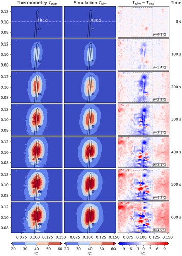
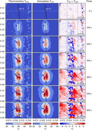
Figure 4. Case 2: Comparison between measured $T_{\exp }$ and simulated temperature $T_{\text{sim}}.$ The standard deviation σ is computed within the dashed box, disregarding the hatched area where the measurement is unreliable due to coagulation. Note: For this case artifacts in the MR thermometry data likely result in faulty temperature measurements.

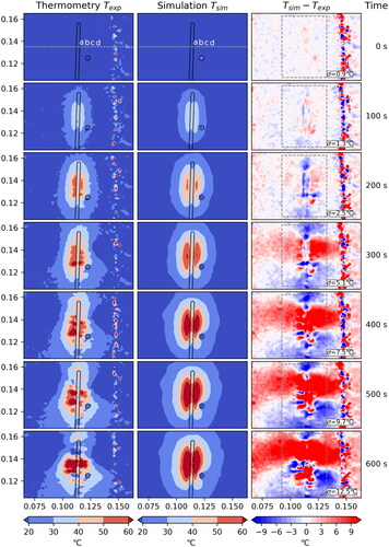
Figure 5. Case 3: Comparison between measured $T_{\exp }$ and simulated temperature $T_{\text{sim}}.$ The standard deviation σ is computed within the dashed box, disregarding the hatched area where the measurement is unreliable due to coagulation.

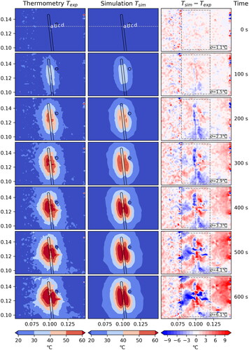
Figure 6. Case 4: Comparison between measured $T_{\exp }$ and simulated temperature $T_{\text{sim}}.$ The standard deviation σ is computed within the dashed box, disregarding the hatched area where the measurement is unreliable due to coagulation. Note: For this case artifacts in the MR thermometry data likely result in faulty temperature measurements.

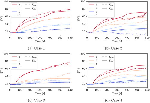
Furthermore, we define four points a, b, c and d with distances 3, 8, 13 and 18 mm to the center of the applicator, respectively. These points are used to compare temperatures over time. Additionally, we define a line to plot a one-dimensional cut through the experimental region. The points as well as the line are highlighted in Figures 3–6.

3. Results

The results for the four experiments Case 1–4 are shown in Figures 3–6, respectively. Each figure shows a comparison between the measured temperature $T_{\exp }$ obtained from MR thermometry in the left column and the simulated temperature $T_{\text{sim}}$ in the middle column from 0 to 600 s into the experiment. For now we limit the comparison to this time window, because afterwards changing tissue properties and increasing vapor transport (not accounted for in the model yet) as well as an increasing drift of the magnetic field become and issue. See Section 4 for a detailed discussion and possible solutions.

The positions of the applicator and the artificial vessel are marked. The right column shows the difference between simulated and measured temperature. Additionally, the standard deviation $\sigma ({\Omega }_R)$ within the active region of the ablation, which is marked by a dashed gray line, is given.

In Figure 7 we compare the measured and simulated temperatures over a line that runs through the middle of the applicator for four different time steps. Moreover, Figure 8 shows the temporal evolution of measured and simulated temperatures at the four points a, b, c, and d.

Figure 7. One-dimensional plot over the line shown in Figures 3–6 to compare measured and simulated temperatures at different time steps during the experiments.

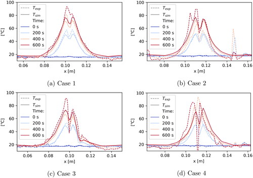
Figure 8. Plot over time at the points a, b, c and d (Figures 3–6) to compare measured and simulated temperatures.

Quantitative results on the influence of the vessel are given in Table 4, where the mean of the measured and simulated temperatures ${\overline{T}}_{\exp }$ and ${\overline{T}}_{\text{sim}}$ as well as the standard deviation σ are given in the regions of interest Ω_V (around the vessel) and Ω_C (contralateral to the vessel).

Table 4. Mean temperatures ${\overline{T}}_{\exp }$ and ${\overline{T}}_{\text{sim}}$ as well as standard deviation σ in regions of interest (ROI) with radius 5 mm around the vessel (Ω_V) and contralateral to the vessel (Ω_C), i.e. around the position of the vessel mirrored by the applicator.

		ROI	0 s	100 s	200 s	300 s	400 s	500 s	600 s
Case1	${\overline{T}}_{\exp }$	ΩV	16.1	21.9	27.4	30.1	30.7	30.3	30.3
		ΩC	16.0	24.8	36.4	41.9	46.3	46.7	48.6
	${\overline{T}}_{\text{sim}}$	ΩV	17.4	23.0	26.1	27.6	28.6	29.2	29.5
		ΩC	16.0	24.4	35.1	41.6	46.0	48.8	50.5
	σ	ΩV	1.7	1.6	3.7	5.4	6.8	8.3	9.4
		ΩC	0.6	1.0	1.2	3.7	7.2	6.5	5.1
Case2	${\overline{T}}_{\exp }$	ΩV	17.7	22.8	29.0	31.8	33.1	34.1	34.3
		ΩC	17.8	23.7	34.4	40.5	46.5	49.6	43.6
	${\overline{T}}_{\text{sim}}$	ΩV	18.4	23.1	26.9	28.7	29.8	30.4	30.7
		ΩC	17.5	23.5	33.7	40.7	45.5	48.1	49.7
	σ	ΩV	1.3	2.1	4.6	4.3	4.1	5.5	7.4
		ΩC	0.7	1.1	1.6	3.2	5.2	6.6	16.4
Case3	${\overline{T}}_{\exp }$	ΩV	17.9	21.6	26.6	29.2	29.9	31.4	32.9
		ΩC	17.5	22.7	33.0	43.2	49.1	53.7	56.9
	${\overline{T}}_{\text{sim}}$	ΩV	18.4	22.9	27.1	29.1	30.4	31.0	31.2
		ΩC	17.5	23.5	34.3	42.0	47.0	49.5	51.1
	σ	ΩV	1.1	1.5	3.0	4.0	5.0	5.5	7.6
		ΩC	1.0	1.2	1.1	1.6	1.9	2.2	3.0
Case4	${\overline{T}}_{\exp }$	ΩV	19.5	26.4	35.8	37.3	36.9	37.2	37.8
		ΩC	18.2	26.0	39.0	43.3	44.1	44.2	45.2
	${\overline{T}}_{\text{sim}}$	ΩV	18.8	25.2	29.6	31.5	33.2	34.3	34.8
		ΩC	18.0	27.3	40.8	49.2	54.9	57.9	59.4
	σ	ΩV	8.5	6.6	11.5	23.9	24.2	31.2	37.1
		ΩC	0.7	1.5	2.9	3.8	3.7	4.7	6.7

A run of the whole simulation pipeline takes about 160 s per case on standard PC hardware. The simulation pipeline consists of preprocessing (geometry and mesh generation), solve of the time-dependent PDE system and postprocessing (generating plots and figures). The solve step alone takes about 40 s. We are using a tetrahedral mesh with about 14,000 elements. If necessary, the pre- and postprocessing steps could be speed up significantly by a more efficient implementation. Making use of parallelization it should also be possible to speed up the solve step by some factor.

4. Discussion

The agreement between measured and simulated temperature is very good for Case 1 (Figure 3) and Case 3 (Figure 5), where we have a standard deviation $\sigma ({\Omega }_R)$ of 4.9 °C and 6.1 °C, respectively, after 600 s. Additionally, the contour lines of the temperatures are very similar. The effect of the artificial vessel is clearly visible and in good agreement between measurement and simulation. The measured data shows minor artifacts which do not cause a problem for the comparison.

For Case 2 (Figure 4) and Case 4 (Figure 6) there seems to be a major problem with the measured data. Figure 4 shows a temperature drift in the thermometry data $T_{\exp }$ which is best observed by the broad red horizontal region in the difference plot. In part, the measured temperature actually decreases, even in distant areas on which the ablation has no influence at all. Furthermore, one observes a vertical line of artifacts probably originating from air sitting between liver and phantoms. A similar effect can be seen in Figure 6. As a consequence, also the computed standard deviations $\sigma ({\Omega }_R)$ are significantly larger, with a value of 12.5 °C and 13.6 °C, respectively, after 600 s. For these reasons, we focus on Case 1 and 3 for the remaining discussion of our results and note that the results for Case 2 and 4 are having the same problems with the thermometry data as described above.

When studying the one-dimensional plots in Figure 7 we again see that, in general, the agreement between measured and simulated data is quite good. For Cases 1 and 3 the curves agree very nicely. Only at the later time steps some deviations occur in close proximity to the applicator. The plot for Case 3 passes through the vessel (at $x\approx 0.11$ m) which also results in some deviation. This suggests that maybe the applicator and vessel models need to be refined. Another reason may be a change in tissue properties at higher temperatures not accounted for in the model. The comparison with thermoemtry data seems to be a powerful tool to further investigate this issue.

The temporal plots in Figure 8 show nearly perfect agreement for Case 1, except for point a. As point a is closest to the applicator, this again suggests that the model may need refinement. For Case 3 the curves agree nicely up to about 350 s into the experiment when they start to deviate. The close proximity of the vessel position might be a possible explanation, which again suggests that the vessel model could require a refinement.

In Table 4 we investigate the vessel model more closely by comparing a region of interest Ω_V around the vessel with the contralateral region Ω_C exactly at the opposite side of the applicator. As one would expect the mean temperatures around the vessel is lower than on the contralateral side. Additionally, the agreement of the mean measured and simulated temperatures in the respective ROIs is quite good. When looking at the standard deviation between measured and simulated temperature, we observe the values are significantly larger around the vessel than in the contralateral region which again suggests that the vessel model may need refinement.

In general, the deviations between measurement and simulation become larger at higher temperatures. To improve the accuracy of the model the following things should be considered: Use a better model for the changing tissue properties [6,23], model the evaporation of water including the transport of vapor [19] and refine the model for the cooling of the applicator as well as the vessel model.

Having error estimates on the thermometry data would help to evaluate its accuracy. The approach from [33] can help to achieve this in the future.

The artifacts encountered in Cases 2 and 4 can result from changes of the magnetic field in the PRF method. A drift of the static magnetic field (B0 drift) can occur at long acquisition times by the scanner system, but its effects influence the whole image and was also corrected in these experiments [12,34,35]. To correct for the drift an additional region of interest (ROI) in the phantom (which was not involved by the heating) was used ([12–15]).

Alt the beginning of the experiments, the temperature of the samples was slightly below room temperature so that a small increase in temperature may also have occurred in the control region. This potential cause for error can easily be fixed in the future by letting the samples adapt to the room temperature.

Since the artifacts are spatially localized and based on the small volume of the liver, susceptibility differences between liver tissue and air may have produced field inhomogeneities during treatment [36]. To reduce these field inhomogeneities, the liver was framed by two agarose gel phantoms (with similar susceptibility as the liver tissue) in the experiments to significantly increase the object volume and thus help stabilize the magnetic field [37,38]. For further optimization, larger gel phantoms that fit the shape of the liver and leave smaller to no air gaps could be chosen as a solution approach. These gel phantoms, which are not optimally adapted to the liver, cause the vertical artifacts due to an air gap. This is presented outside the dashed box in Figures 3–6 and is therefore not taken into account when calculating the standard deviation.

Another limitation is the high temperatures ($>{100}^{°}$C) which arise during LITT and the associated gas evolution in the liver. The gases can disperse in the empty vessels of the ex-vivo liver and lead to incorrect phase values for temperature calculation [36]. This problem mainly exists for ex-vivo experiments where the liver is not perfused. One approach could still be the use of a water bath to fill the liver vessels with water and avoid gas dispersion. However, a water bath in an MR scanner would lead to motion artifacts in the imaging, since the scanner vibrates slightly during the measurements.

5. Conclusion

In this paper, we have investigated the validation of ex-vivo laser induced thermotherapy (LITT) simulations with the help of MR-thermometry data. We presented a mathematical simulation model for LITT and described the experimental setup used to validate our model. Four experiments were carried out, and the temperature measurements obtained from thermometry were found to be very suitable for validating simulation results and identifying missing parameters. Apart from the likely measurement errors in Cases 2 and 4, the data is of high quality and plausible. The resolution of the data is sufficiently high to resolve even small details such as the influence of the artificial blood vessel on the temperature distribution. Simulation results were in good agreement with measurements and it was possible to identify missing parameters from the data. Altogether, thermometry is a powerful tool to validate and improve simulation models, in particular, since measurements are not restricted to pre-selected points, but are available throughout the entire imaging plane.

Disclosure statement

No potential conflict of interest was reported by the author(s).

Additional information

Funding

This work was supported by the Federal Ministry of Education and Research of Germany (BMBF) under [Grant 05M16AMA].

References

- Paul A, Narasimhan A, Kahlen FJ, et al. Temperature evolution in tissues embedded with large blood vessels during photo-thermal heating. J Therm Biol. 2014;41:77–87.
- Puccini S, Bär N-K, Bublat M, et al. Simulations of thermal tissue coagulation and their value for the planning and monitoring of laser-induced interstitial thermotherapy (litt). Magn Reson Med. 2003;49(2):351–362.
- Mohammed Y, Verhey JF. A finite element method model to simulate laser interstitial thermo therapy in anatomical inhomogeneous regions. Biomed Eng Online. 2005;4(1):2.
- Fasano A, Hömberg D, Naumov D. On a mathematical model for laser-induced thermotherapy. Appl Math Modell. 2010;34(12):3831–3840.
- Hübner F, Leithäuser C, Bazrafshan B, et al. Validation of a mathematical model for laser-induced thermotherapy in liver tissue. Lasers Med Sci. 2017;32(6):1399–1409.
- Bianchi L, Cavarzan F, Ciampitti L, et al. Thermophysical and mechanical properties of biological tissues as a function of temperature: a systematic literature review. Int J Hyperthermia. 2022;39(1):297–340.
- Rossmann C, Haemmerich D. Review of temperature dependence of thermal properties, dielectric properties, and perfusion of biological tissues at hyperthermic and ablation temperatures. Crit Rev Biomed Eng. 2014;42(6):467–492.
- Bazrafshan B, Koujan A, Hübner F, et al. A thermometry software tool for monitoring laser-induced interstitial thermotherapy. Biomed Tech. 2019;64(4):449–457.
- Bazrafshan B, Hübner F, Farshid P, et al. Magnetic resonance temperature imaging of laser-induced thermotherapy: assessment of fast sequences in ex vivo porcine liver. Future Oncol. 2013;9(7):1039–1050.
- Bazrafshan B, Hübner F, Farshid P, et al. Temperature imaging of laser-induced thermotherapy (litt) by MRI: evaluation of different sequences in phantom. Lasers Med Sci. 2014;29(1):173–183.
- Rieke V, Butts Pauly K. MR thermometry. J Magn Reson Imaging. 2008;27(2):376–390.
- Kägebein U, Speck O, Wacker F, et al. Motion correction in proton resonance frequency–based thermometry in the liver. Top Magn Reson Imaging. 2018;27(1):53–61.
- Kickhefel A, Rosenberg C, Weiss CR, et al. Clinical evaluation of mr temperature monitoring of laser-induced thermotherapy in human liver using the proton-resonance-frequency method and predictive models of cell death. J Magn Reson Imaging. 2011;33(3):704–12712.
- Kickhefel A, Rosenberg C, Roland J, et al. A pilot study for clinical feasibility of the near-harmonic 2d referenceless prfs thermometry in liver under free breathing using mr-guided litt ablation data. Int J Hyperthermia. 2012;28(3):250–266.
- Rosenberg C, Kickhefel A, Mensel B, et al. Prfs-based mr thermometry versus an alternative t1 magnitude method–comparative performance predicting thermally induced necrosis in hepatic tumor ablation. PLoS One. 2013;8(10):e78559.
- Pennes HH. Analysis of tissue and arterial blood temperatures in the resting human forearm. J Appl Physiol. 1948;1(2):93–122.
- Niemz MH, et al. Laser-tissue interactions. Springer, Berlin Heidelberg, 2007.
- Modest MF. Radiative heat transfer. Academic Press, San Diego, 2003.
- Blauth S, Hübner F, Leithäuser C, et al. Mathematical modeling of vaporization during laser-induced thermotherapy in liver tissue. J Math Ind. 2020;10:1–16.
- Wu X, Zhang K, Chen Y, et al. Theoretical and experimental study of dual-fiber laser ablation for prostate cancer. PLOS One. 2018;13(10):e0206065.
- Guntur SR, Lee KI, Paeng D-G, et al. Temperature-dependent thermal properties of ex vivo liver undergoing thermal ablation. Ultrasound Med Biol. 2013;39(10):1771–1784.
- Mohammadi A, Bianchi L, Asadi S, et al. Measurement of ex vivo liver, brain and pancreas thermal properties as function of temperature. Sensors. 2021;21(12):4236.
- Mohammadi A, Bianchi L, Korganbayev S, et al. Thermomechanical modeling of laser ablation therapy of tumors: sensitivity analysis and optimization of influential variables. IEEE Trans Biomed Eng. 2022;69(1):302–313.
- Geuzaine C, Remacle J-F. Gmsh: a 3-D finite element mesh generator with built-in pre- and post-processing facilities. Int J Numer Meth Engng. 2009;79(11):1309–1331.
- Alnaes MS, Blechta J, Hake J, et al. The fenics project version 1.5. Arch Numer Software. 2015;3(100):9–23.
- Logg A, Mardal K-A, Wells GN, et al. Automated solution of differential equations by the finite element method. Heidelberg: Springer; 2012.
- Balay S, Abhyankar S, Adams MF, et al. PETSc users manual (technical report ANL-95/11 – Revision 3.11). Lemont (IL): Argonne National Laboratory; 2019.
- Andres M, Blauth S, Leithäuser C, et al. Identification of the blood perfusion rate for laser-induced thermotherapy in the liver. J Math Ind. 2020;10:1–20.
- Roggan A, Dorschel K, Minet O, et al. The optical properties of biological tissue in the near infrared wavelength range. In Laser-induced interstitial therapy. Bellingham (WA): SPIE Press; 1995. p. 10–44.
- Giering K, Minet O, Lamprecht I, et al. Review of thermal properties of biological tissues. In Laser-induced interstitial therapy. Bellingham (WA): SPIE Press; 1995. p. 45–65.
- Schwarzmaier H-J, Yaroslavsky IV, Yaroslavsky AN, et al. Treatment planning for mri-guided laser-induced interstitial thermotherapy of brain tumors–the role of blood perfusion. J Magn Reson Imaging. 1998;8(1):121–127.
- Byrd RH, Lu P, Nocedal J, et al. A limited memory algorithm for bound constrained optimization. SIAM J. Sci. Comput. 1995;16(5):1190–1208.
- Fuentes D, Yung J, Hazle JD, et al. Kalman filtered mr temperature imaging for laser induced thermal therapies. IEEE Trans. Med. Imaging. 2012;31(4):984–994.
- Poorman ME, Braškutė I, Bartels LW, et al. Multi-echo mr thermometry using iterative separation of baseline water and fat images. Magn Reson Med. 2019;81(4):2385–2398.
- Odéen H, Parker DL. Magnetic resonance thermometry and its biological applications–physical principles and practical considerations. Prog Nucl Magn Reson Spectrosc. 2019;110:34–61.
- Kuroda K. Mr techniques for guiding high-intensity focused ultrasound (hifu) treatments. J Magn Reson Imaging. 2018;47(2):316–331.
- Saccomandi P, Schena E, Silvestri S. Techniques for temperature monitoring during laser-induced thermotherapy: an overview. Int J Hyperthermia. 2013;29(7):609–619.
- Hübner F, Bazrafshan B, Roland J, et al. The influence of nd: Yag laser irradiation on fluoroptic[textregistered] temperature measurement: an experimental evaluation. Lasers Med Sci. 2013;28(2):487–496