The hot-to-cold spot quotient for SAR-based treatment planning in deep microwave hyperthermia

Abstract

Background

A necessary precondition for a successful microwave hyperthermia (HT) treatment delivered by phased arrays is the ability of the HT applicator to selectively raise the temperature of the entire tumor volume. SAR-based treatment plan (HTP) optimization methods exploit the correlation between specific absorption rate (SAR) and temperature increase in order to determine the set of steering parameters for optimal focusing, while allowing for lower model complexity. Several cost functions have been suggested in the past for this optimization problem. However, their correlation with high and homogeneous tumor temperatures remains sub-optimal in many cases. Previously, we proposed the hot-to-cold spot quotient (HCQ) as a novel cost function for SAR-based HTP optimization and showed its potential to address these issues.

Materials and methods

In this work, we validate the HCQ on a standard ESHO patient repository within single and multi-frequency contexts. We verify its correlation with clinical SAR and temperature indexes, and compare it to HTPs obtained using a commonly accepted cost-function for SAR-based HTP (hot-spot to target quotient, HTQ).

Results and discussion

The results show that low HCQ values produce better SAR (TC₅₀, TC₇₅) and temperature metrics (T₅₀, T₉₀) than HTQ in most patient models and frequency settings. For the deep-seated tumors, the correlation between the clinical indicators and 1/HCQ is more favorable than the correlation exhibited by 1/HTQ.

Conclusion

The validation confirms the ability of HCQ to promote target coverage and hot-spot suppression in SAR-based HTP optimization, resulting in higher SAR and temperature indexes for deep-seated tumors.

Keywords:

• Hyperthermia
• computational modeling
• treatment planning
• cost function
• control systems engineering/treatment optimization
• SAR
• radiofrequency/microwave
• temperature

1. Introduction

In deep microwave hyperthermia (HT) cancer treatment, the tumor temperature is elevated to 40–44 °C for about an hour by a conformal array of antennas called applicator [1,2]. This adjuvant therapy has been shown to enhance the tumor response and survival rate of cancer patients in many clinical trials [3–5]. The antennas radiate coherently at one or more frequencies with different amplitude and phase to generate a focalized power deposition pattern. The aim of the treatment is to reach a therapeutic temperature range in the target volume while not exceeding thermal toxicity thresholds for (nearby) healthy tissues [6,7].

To this end, a preliminary HT treatment planning (HTP) step is prescribed by current guidelines [8]. In this stage, the set of optimal steering parameters (amplitude and phase) for each antenna is determined by means of numerical simulations involving a segmented model of the patient and a model of the applicator in use [9]. Iterative optimization algorithms explore the space of possible solutions and determine the one that minimizes a certain cost function. As the aim of the treatment is to reach and maintain a therapeutic temperature in the target volume for a specified duration, the goal of the optimization should ideally be the temperature itself. To date, a few in-house built and commercial HTP optimization software packages offer the possibility to carry out thermal simulations and optimizations [10]. Thermal HTP can be particularly effective when large blood vessels are present in the vicinity of the tumor [11,12], as these extract a large amount of heat. Thermal simulations can further account for heat redistribution due to convection [13]. These benefits are unfortunately overshadowed in clinical practice by the additional segmentation needed to include vasculature and the longer computation times. A practical solution to obtain a good plan with limited model complexity is to use the specific absorption rate (SAR) distribution as a surrogate to the temperature distribution, thanks to its correlation to the temperature increase [14] and treatment outcome [15]. As a matter of fact, both SAR- and temperature-based HTP optimizers are currently in use in the clinical setting, as both require online adjustments during treatment [16,17]. One clear advantage of SAR, however, is its faster computation speed, which becomes particularly helpful in the case of multi-frequency plans, where the number of variables subject to optimization increases linearly with the number of frequencies considered.

The HTP optimization process should lead to high and homogeneous tumor temperatures for a set temperature limit in the healthy tissues. In general, the temperature increase in the patient during treatment is known to be limited by the occurrence of hot-spots [18]. A hot-spot is defined as a localized temperature increase outside the target volume, and can result in pain and discomfort for the patient, but also induces thermal toxicity in healthy tissue. When a hot-spot is reported by the patient or detected by thermal probes, the power of the applicator device has to be lowered or redistributed to different channels [16,17]. Consequently, the temperature achievable in the tumor will be constrained by the maximum power than can be radiated into the patient without causing hot-spots. The location and severity of hot-spots is not straightforward to predict, because they arise from the inhomogeneity of the patient anatomy together with the finite aperture of the applicator array and its steering settings.

In SAR, hot-spots are detectable as local power deposition peaks [14]. As such, they can be addressed during the HTP optimization stage. This is a well-known problem that has been tackled in various ways [19]. Some approaches make use of convex programming to shape the SAR according to some (constrained) quadratic criterion [20–23]. While direct and exact, these methods need to make assumptions on the predicted location and intensity of the SAR peaks to assemble the constraint mask. This might lead to sub-optimal solutions as the SAR peaks depend on the steering solution itself, and their tracking is better achieved by non-linear operators [24], which however cannot be solved for directly. In fact, the current practice in SAR-based optimization relies on the non-linear hot-spot to target quotient (HTQ) [25]. The HTQ identifies the hot-spot(s) as the highest first percentile of the SAR distribution outside the target. The percentile sub-volume needs to be recomputed for each solution, requiring an iterative procedure. By minimizing the HTQ, the average SAR deposition in the tumor increases while the most prominent hot-spot in the healthy tissues is suppressed.

Despite their prominent role in HTP, hot-spots represent only part of the challenge in HT heating. The second fundamental element of a successful treatment is the homogeneity of the thermal dose administered to the tumor, which can be expressed in terms of the minimum temperature achieved in the target [26]. Ideally, all regions of the delineated target volume should reach 43 °C for the treatment to be effective. This condition, however, is not directly addressed by the definition of HTQ, because its denominator is a mere average of the SAR values across the whole target, which implicitly neglects the inhomogeneities in SAR deposition. As a result, some areas of the tumor, so called cold-spots, may remain untreated as they fail to reach the prescribed thermal dose. A low correlation between 1/HTQ and the temperature achieved by at least 90% of the target volume (T₉₀) supports this concern [27]. Due to the paramount importance of the T₉₀ metric, which has been shown to directly correlate with clinical outcome [28], it is crucial that SAR-based optimizations yield HTPs that strive for the highest possible T₉₀.

To this end, we have recently proposed a novel cost function for SAR-based HTP optimization, the hot-to-cold spot quotient (HCQ) [29]. Together with hot-spots in healthy tissues, this cost function also identifies cold-spots in the target volume as the average SAR in the lowest percentile. The definition of the healthy tissue and tumor percentiles in HCQ makes the values obtained from different HTPs and patients quantitatively comparable. Our preliminary data indicated that HCQ is capable of yielding treatment plans exhibiting a good compromise between hot-spot suppression (low HTQ) and target coverage (high TC₂₅, [15]) than conventional SAR-based optimizations.

The aim of this study is to validate the HCQ as goal function for the optimization of single and multi-frequency HTP on a set of six patient models that cover some of the most common HT treatment sites. The models have been made publicly available by the Erasmus Medical Center (EMC, Rotterdam, The Netherlands) via the European Society of Hyperthermic Oncology (ESHO) [30,31]. We benchmark the SAR and temperature distributions of the HCQ-optimal plans against the plans obtained by optimizing for the conventional cost function, the HTQ. We further investigate the sensitivity of the HCQ metric to the percentile value for hot- and cold-spot identification. Finally, we compare the correlation of 1/HCQ and 1/HTQ with clinical SAR (TC₅₀, TC₇₅) and temperature (T₅₀, T₉₀) indicators.

2. Method

In the following subsections, we describe in detail the validation protocol from patient and applicator modeling to the quantitative assessment of the thermal distributions.

2.1. Patient models

Six representative patient models have recently been prepared as a means for standardization in HTP development, validation and comparison [31]. The models include two head and neck patients, one with a nasopharyngeal tumor (Alex) and one post-operative oropharyngeal case (Murphy) with metal dental implants. Two breast models represent patients with a superficial tumor (Venus) and a deep-seated tumor (Luna). The last two models are for pelvic targets and include a rectal (Will) and a cervical (Clarice) case. All models are shown in Figures 1 and 2.

The models are provided as already segmented volume matrices. The head and neck models are segmented into 16 biological tissues (tumor, muscle, fat, sclera, vitreous humor, optical nerve, spinal cord, cartilage, eye lens, cerebrum, cerebellum, cartilage, brain stem, thyroid, bone and lung) plus internal air and metal implants where applicable. The breast models are segmented into six tissues (tumor, bone, breast gland, skin, muscle and fat) and exhibit no internal air lumina. The pelvis models are segmented into four tissues (tumor, muscle, fat and bone) plus internal air.

The three body sites are sampled with different resolutions: the head and neck models have a resolution of 2.5 mm, the pelvis models 5.0 mm and the breast models 1.0 mm. To reduce the computational burden, we down-sample the breast models to 2.0 mm using a winner-takes-all strategy [32], in line with the recommendations of the reference paper for the dataset [31].

2.2. Tissue properties

Material properties are retrieved from the IT’IS database [33] for each healthy tissue in the dataset, as prescribed by the reference paper [31]. The properties include density (ρ, [kg/m³]), dispersive relative permittivity (ϵ, [1]) and dispersive conductivity (σ, [S/m]), specific heat capacity (c_p, [J/kg/K]), thermal conductivity (κ, [W/m/K]), heat transfer rate (q_t, [ml/min/kg]), and heat generation rate (Q_g, [W/kg]). All thermal properties are taken under normothermic conditions.

Dispersive dielectric tumor properties are obtained as an average of all malignant tissue properties reported by Joines et al. [34], as recommended by Paulides et al. [31]. Other tumor properties are taken directly from the reference paper [31]: ρ= 1090 [kg/m³], c_p = 3421 [J/kg/K] and κ= 0.49 [W/m/K]. The paper does not provide details regarding the origin of these values. The given heat transfer rate under thermal stress for the tumor is q_t=94.4 [ml/min/kg].

2.3. Applicator design

Customized array applicators are designed for each patient. Two topologies are employed: cylindrical for neck and pelvis models, semi-spherical for breast models. The applicators utilize ultra wide-band (UWB) self-grounded bow-tie antennas [35], and the operating frequency band is selected for each target region according to the expected focal size and penetration depth [36–38]. In particular, the band is 400–800 MHz for the neck models, 500–1000 MHz for the breast models and 150–300 MHz for the pelvis models. The antennas are immersed in a water bolus which encloses the target body region, to achieve dielectric matching and implement skin cooling. The thickness of the water bolus, defining also the distance of the antenna ground plane to the body, is 5 cm for the neck models, 4 cm for the breast models and 12 cm for the pelvis models.

Since the scope of this study is limited to the evaluation and comparative assessment of the HCQ in HTP optimization, we summarize only in brief the design procedure of the applicators:

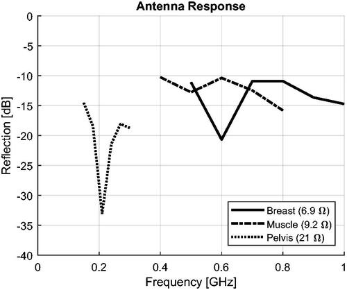
1. Optimize the antenna proportions to provide a good response and radiation pattern across the intended operating octave. Figure 3 shows the resulting geometries and Figure 4 reports the reflection coefficient of each antenna (S11 normalized to the reported real impedance).

2. Obtain the bolus dimensions by fitting an ellipsoidal cylinder or sphere over the shape of the target body region, maintaining as much a possible the specified bolus thickness.

3. Construct the antenna array by inserting as many antennas as possible while respecting the minimum distance between antennas to limit cross coupling.

Figure 1. Schematic of the patient models and the applicator. The water bolus is shown in blue. The patient model is shown in gray. (a) and (b) show the 14-channel two-row cylindrical applicator for Alex. (c) and (d) show the 16-channel two-row cylindrical applicator for Murphy. (e) and (f) show the 10-channel spherical applicator for Venus.

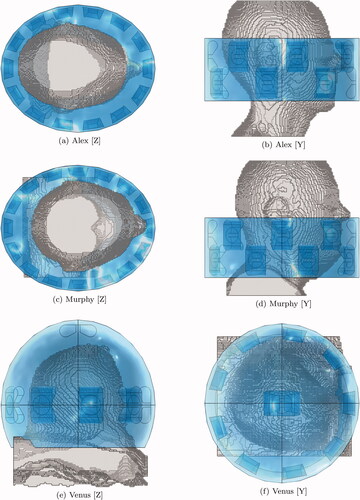
Figure 2. Schematic of the patient models and the applicator. The water bolus is shown in blue. The patient model is shown in gray. (a) and (b) show the 8-channel spherical applicator for Luna. (c) and (d) show the 14-channel two-row cylindrical applicator for Will. (e) and (f) show the 14-channel two-row cylindrical applicator for Clarice.

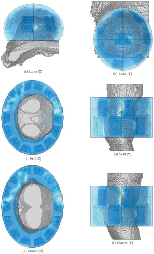
Reiterating the design procedure for each patient model results in six applicators, as illustrated in Figures 1 and 2. Each applicator has a different number of antennas (Alex = 14, Murphy = 16, Luna = 8, Venus = 10, Clarice = 14, Will = 14). While the personalization of the applicator array might be impracticable in the clinical setting, it provides us with a heterogeneous set of test cases for a more robust assessment of the HTP optimization in different setups.

Figure 3. Antenna models utilized to assemble the applicators at the three selected operating bands. The illustrations are not to scale, in order to highlight the relative differences. (a) and (b) show the geometry optimized for a pelvis phantom, length 15.2 cm. (c) and (d) show the geometry optimized for a muscle phantom, length 6 cm. (e) and (f) show the geometry optimized for a breast phantom, length 5 cm.

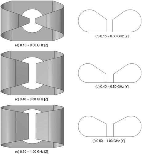
Figure 4. Reflection coefficients of the antenna models calculated at their (real) radiation impedance. The impedance is shown in the legend.

2.4. Electromagnetic simulations

Electromagnetic simulations are performed in COMSOL Multiphysics^®, a FEM-based commercial software [39]. Mesh resolutions vary from λ/20 in proximity of the metal antenna parts, to λ/5 in regions far from the peak field gradients, where λ is the wavelength at the highest operating frequency. The patient models are uploaded in the COMSOL project after converting the volumetric tissue masks to CAD shapes. The three-dimensional distributions of the material properties inside the patient are captured by custom space-varying functions. Air is modeled as vacuum, while distilled water is modeled as a dispersive first-order Debye model. The surface of metal implants is treated as perfect electric conductor. At the domain boundaries, absorbing conditions (PML) are defined.

At this simulation stage, the E-field distributions inside the patient are calculated for each antenna at each operating frequency. We solve for three frequency points for each patient, which are minimum, maximum and center frequency within the applicator’s operating band. Thus, the frequency sweep is [400, 600, 800] MHz for the neck models, [500, 750, 1000] MHz for the breast models and [150, 225, 300] MHz for the pelvis models.

2.5. Treatment planning

The SAR-based HTP optimization is carried out for each model to produce single and multi-frequency treatment plans. The plans are obtained at the minimum, the center and the maximum frequency, and at binary combinations of these, for a total of six operating frequency settings. The optimization setup is identical for all patients, and for the comparative analysis we alter only the cost function.

The HCQ is the goal we propose for SAR-based HTP-optimization, and is defined as follows [29]: (1) $${\text{HCQ}}_{\mathrm{p}}=\frac{{\overline{\text{SAR}}}_{{\mathrm{R}}_{\mathrm{q}}}}{{\overline{\text{SAR}}}_{{\mathrm{T}}_{\mathrm{p}}}}$$(1) where SAR_Tp is the average SAR in the lowest p-percentile of target (tumor) tissue, while SAR_Rq is the average SAR in the highest q-percentile of remaining (healthy) tissue. To render the HCQ metric comparable between different patients and targets, the percentiles are related as follows: (2) $$\mathrm{q}=\mathrm{p}\frac{\left|\mathrm{T}\right|}{\left|\mathrm{R}\right|}$$(2) where ǁ denotes the volume of the argument (T target, R remaining). This relationship results in the hot- and cold-spot masks having the same volume p·|T|, as shown in Figure 5. As one of the aims of this study is to determine the optimal target percentile p, we let p vary from 1% (the SAR value at the single point of minimum inside the target) to 99% (the average of all SAR values inside the target) and obtain HTPs and corresponding thermal distributions for a range of values in between these extremes.

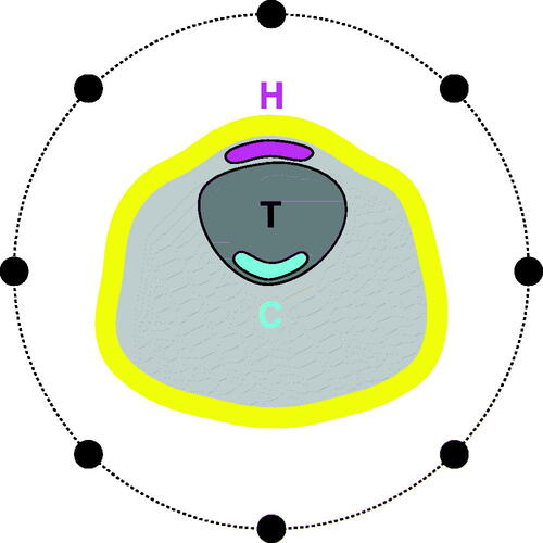
Figure 5. Illustrating the hot-spot (H, magenta) and cold-spot (C, cyan) sub-volumes. Schematic of neck section with target volume T and a ring applicator (black dots). Both H and C are equal to a fraction p of the target volume. The first centimeter of skin (yellow) is excluded from the spot evaluation. Note that the hot- and cold-spot sub-volumes are not necessarily contiguous sub-sets of the target T and the remaining tissue R, respectively.

The benchmark cost function for SAR-based HTP-optimization is the HTQ, defined as follows [14]: (3) $$\mathrm{HTQ}=\frac{{\overline{\text{SAR}}}_{\mathrm{R}1}}{{\overline{\text{SAR}}}_{\mathrm{T}}}$$(3) where SAR_R1 is the average SAR in the highest 1-percentile of remaining (healthy) tissue, while SAR_T is the average SAR in the target (tumor) tissue. The HTQ, however, is not a set standard. Recently, a modification has been suggested to fix the hot-spot size to 50 ml to address scaling issues [27,31]. Nevertheless, the form (3) remains the most characterized in the literature and we therefore use it for the comparison. For completeness, we report in Appendix A a second set of treatment plans obtained by fixing the hot-spot size to 50 ml (HTQ’). The correlation of 1/HTQ’ with the SAR indices is lower, while the correlation with the temperatures indices is higher. The absolute target coverage and temperatures; however, become lower on average. As the fixed hot-spot modification does not fundamentally alter the behavior of HTQ, we hereon consider only the classic definition (3).

The optimization process determines the set of steering parameters that minimizes the value of the cost function when evaluated over a patient model. Upon evaluation, the steering parameters are applied to the individual E-fields computed by the FEM solver, and the total array field at frequency f is determined by superposition: (4) $${\mathrm{E}}_{\mathrm{f}}(\mathrm{x},\mathrm{ }\mathrm{y},\mathrm{ }\mathrm{z}\mathrm{)}=\sum _{\mathrm{c}}{\mathrm{p}}_{\mathrm{f},\mathrm{c}}{\mathrm{E}}_{\mathrm{f},\mathrm{c}}\mathrm{(}\mathrm{x},\mathrm{ }\mathrm{y},\mathrm{ }\mathrm{z}\mathrm{)}$$(4) where p_f,c and E_f,c are the complex steering parameter and E-field distribution relative to channel c at frequency f.

The conversion to SAR is carried out in MATLAB^® [40] according to the following: (5) $$\text{SAR}\mathrm{(}\mathrm{x},\mathrm{ }\mathrm{y},\mathrm{ }\mathrm{z})=\sum _{\mathrm{f}}\frac{1}{2}\frac{{\mathrm{\sigma }}_{\mathrm{f}}\mathrm{(}\mathrm{x},\mathrm{ }\mathrm{y},\mathrm{ }\mathrm{z}\mathrm{)}}{\mathrm{\rho }\mathrm{(}\mathrm{x},\mathrm{ }\mathrm{y},\mathrm{ }\mathrm{z}\mathrm{)}}{\parallel {\mathrm{E}}_{\mathrm{f}}\mathrm{(}\mathrm{x},\mathrm{ }\mathrm{y},\mathrm{ }\mathrm{z}\mathrm{)}\parallel }^2$$(5) where E_f is the focused E-field distribution obtained above. The SAR distribution is further convoluted to an averaging spherical kernel of varying size. At each point, the size of the kernel is expanded until it covers 1 g of patient tissue, excluding anything that is not patient. Thus, at the patient surface, water from the bolus and air from the background are excluded from the averaging process.

In the evaluation of the SAR distribution, we exclude the first centimeter of patient surface that is in direct contact with the water bolus. This allows us to model the cooling effect of the water bolus, which effectively extracts heat from the skin and counteracts the high SAR deposition in the first layers of tissue [41]. This step is realized by expanding the bolus mask in the 3D matrix model with a morphological operation using a spherical kernel of radius 1 cm. Consequently, the skin surface that is in contact with air is not subjected to this exclusion.

The optimization problem is solved using the particle swarm global minimization algorithm [42]. The algorithm is configured to solve for a vector of variables composed of amplitude and phase for each channel and for each frequency, for a total of n_v = 2·n_c ·n_f variables, where n_c is the number of channels and n_f is the number of frequencies. As the complexity of the optimization landscape increases with the number of dimensions (variables), we set the number of particles to n_v to attain the same likelihood of finding the global minimum regardless of the problem size [43]. The algorithm is halted when the relative change in the cost value falls below 1% for n_v consecutive iterations. Naturally, treatment plans considering multiple frequencies require longer computation times than single-frequency ones. The solution is further refined using a local gradient descent (lsqnonlin). All algorithms are readily available in MATLAB. To speed up the computations, the SAR calculations are performed in single precision on a high-speed GPU. With the above settings, the optimizations take on average the times reported in Table 1. The HCQ plans require slightly more computation time than the HTQ ones. The increased time is not due to a greater computational complexity, but to the higher number of iterations needed to converge (not shown).

Table 1. Average computation times for HTQ and HCQ₃₀ in single- and multi-frequency settings.

	HTQ	HCQ30
Single frequency	85 s	129 s
Dual frequency	487 s	677 s

Measured on a 24-core Intel Xeon 2.6 GHz. The SAR matrix computations are performed on a nVidia Quadro RTX 6000.

2.6. Thermal simulations

Thermal simulations are also carried out in COMSOL Multiphysics^®, but with domain restricted to the biological tissues only. The mesh resolution is set to vary from r/3 at material interfaces to r·3 in the material bulks, where r is the patient model resolution.

The heat transfer rate q_t [ml/min/kg] is converted to blood perfusion rate ω_b [1/s] using the known value of tissue density. A similar transformation is done to obtain the basal metabolic rate Q_m [W/m³] from the available heat generation rate Q_g [W/kg]. For the metal implants in Murphy, we utilize the mechanical and thermal properties of the titanium alloy Ti-6 Al-4 V, solid and oxidized at 816 °C, as this is one of the most common solutions for dental implants [44]. The thermal properties of this alloy at 43 °C are: ρ = 4428 [kg/m³], c_p = 547 [J/kg/K], κ = 7.2 [W/m/K].

At the interface between patient and air or water, heat flux boundary conditions modeling the convective extraction of heat are implemented. The chosen convection coefficient for skin/air is 8 W/m[²/K] [45], while the coefficient for skin/water is 100 [W/m²/K] [41]. In all test cases, both the air and the water temperatures are set to 20 °C.

The external heat source, or power loss distribution (PLD), is prepared by applying the steering parameters according to the HTP: (6) $$\text{PLD}\mathrm{(}\mathrm{x},\mathrm{ }\mathrm{y},\mathrm{ }\mathrm{z}\mathrm{)}=\sum _{\mathrm{f}}\frac{1}{2}\mathrm{\sigma }\left(\mathrm{x},\mathrm{y},\mathrm{z},\mathrm{f}\right){\parallel \mathrm{E}\left(\mathrm{x},\mathrm{y},\mathrm{z},\mathrm{f}\right)\parallel }^2$$(6)

The relationship between SAR and PLD is straightforward. However, the PLD matrix is not manipulated with mass averaging or surface exclusion. The PLD distribution is iteratively scaled until the maximum temperature in the remaining (healthy) tissue reaches 43 °C as a conservative limit to prevent thermal damage [6], also considering the known wide uncertainties between simulated and measured temperatures (≈2 °C) [46].

2.7. Evaluation metrics

We quantitatively assess the SAR and temperature distributions for each HTP. According to clinical practice, tumor coverage is evaluated by the indexed temperatures T₅₀ and T₉₀ metrics [8], which represent the lowest temperature achieved in the highest 50% and 90% of the target volume, respectively. These metrics have been shown to directly correlate with clinical outcome [47].

In SAR-based assessment, we evaluate the iso-contour target coverage (TC_n) for n = 50% and n = 75%, defined as: (7) $${\text{TC}}_{\mathrm{n}}=\frac{\left|{\mathrm{T}}^{\prime }\right|}{\left|\mathrm{T}\right|}\left[\mathrm{\%}\right],{\mathrm{T}}^{\prime }\mathrm{}|\mathrm{}\text{SAR}\left({\mathrm{T}}^{\prime }\right)\hspace{0.17em}\ge \hspace{0.17em}\mathrm{n}·\text{SAR}\left(\mathrm{R}\cup \mathrm{T}\right)$$(7)

that is, the fraction of target volume subjected to SAR values greater than a fraction n of the maximum SAR peak in the whole patient. The TC₂₅ metric has been shown to be a prognostic factor for local control in HT [15], while the TC₅₀ metric has been shown to correlate with the clinical temperature indicators T₅₀ and T₉₀ in the head and neck [27]. In this study, due to the extensive SAR processing consisting of both averaging and exclusion of surface layers, the SAR distributions do not exhibit sharp peaks nor strong gradients. Typically, the highest SAR values can be found in the first layer of tissue where the energy losses of the incident wave are the strongest. Exclusion of this layer leads to the reduction of the overall detected SAR peak by orders of magnitude, as the wave attenuates exponentially while penetrating the tissue. The additional mass-smoothing further dampens the deeper SAR peaks. Because of this, the resulting SAR values in the target volume become easily higher than 25% of the overall SAR peak. Consequently, the TC₂₅ metric (and TC₅₀ in the breast models) saturates at 100% for most plans. Therefore, we report values of target coverage only for the 50% or 75% of the peak SAR depending on which one is most informative.

2.8. Correlation analysis

In total, 36 treatment plans (6 patients, 6 frequency combinations) are obtained for each cost function definition. On these evaluation points, we carry out a correlation analysis between the inverse of the cost value (1/HTQ, 1/HCQ) and each HTP quality indicator (TC₅₀, TC₇₅, T₅₀ and T₉₀). The metric is the standard Pearson’s correlation coefficient r.

3. Results

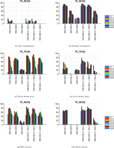
The values of the SAR indicator TC are reported for all patients and treatment plans in Figure 6. As this metric varies widely and saturates for different patients regardless of the cost function used for optimization, we report the value at the fraction that is most relevant for the tumor site. The single-frequency plans exhibit a clear frequency dependent trend. Within the studied bands, the lowest frequency yields best coverage, even in smaller tumors (Venus). The addition of a second frequency is beneficial in Venus, Luna and Clarice, especially when HCQ is used as cost function. Overall, the HCQ optimal solutions yield systematically higher coverage than the HTQ optimal ones, except in Alex. However, the selection of the percentile p has a strong impact on the overall performance of HCQ. Low percentile values yield higher coverage with the maximum coverage often achieved at the lowest value of p = 1%.

Figure 6. Treatment plan values of target coverage (SAR) for each patient, frequency combination, and optimization cost function. The cost function is color-coded in the legend. (a), (b), (g), and (h) report values of TC₅₀ for the neck and pelvis models. (d) and (e) report values of TC₇₅ for the breast models, as TC₅₀ saturates at 100% for these patients.

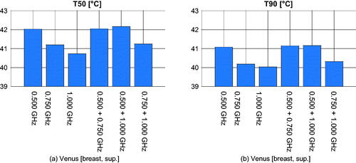
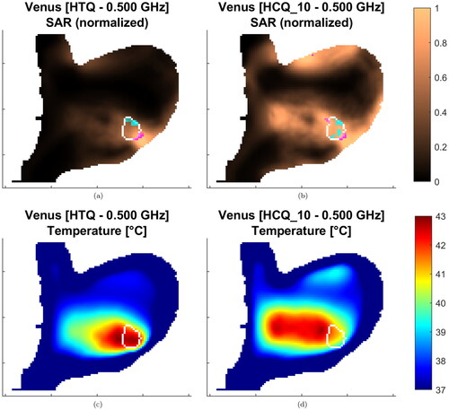
The values of the T₅₀ and T₉₀ indicators for the resulting temperature distributions are presented in Figures 7 and 8. The temperature variations highlight the heterogeneity of the patient dataset. In a similar way as in the SAR analysis, the HCQ-based HTPs perform equally or better than the HTQ ones. As an example, the SAR and temperature distributions for Alex in a multi-frequency HTP are shown in Figure 9. The HCQ extends the SAR deposition to cover the entire target, which leads to higher tumor temperatures. The SAR distributions of the individual frequencies support the homogeneous heating with complementary patterns (not shown). One notable exception in the set is the superficial breast tumor in Venus. The SAR and thermal distributions of both HTQ and HCQ plans for this patient are illustrated in Figure 10. The SAR distribution after HCQ optimization is more homogeneous than in the HTQ case. However, the heating pattern is affected by the proximity of the water bolus. HTQ is favored by this mechanism and achieves almost 1.5 °C higher T than the HCQ solution. In all remaining cases, HCQ yields temperature indexes up to half a degree higher than the HTQ solution, and is particularly beneficial in Alex and Will with almost 1 °C higher T₉₀.

Figure 7. Treatment plan values of 50-percentile tumor temperature (T₅₀) for each patient, frequency combination, and optimization cost function. The cost function is color-coded in the legend. The maximum temperature anywhere in the healthy tissues is 43 °C.

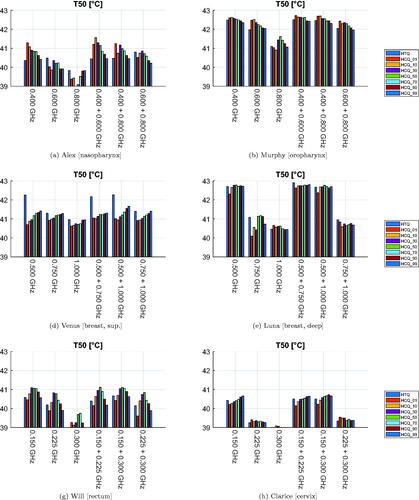
Figure 8. Treatment plan values of 90-percentile tumor temperature (T₉₀) for each patient, frequency combination, and optimization cost function. The cost function is color-coded in the legend. The maximum temperature anywhere in the healthy tissues is 43 °C.

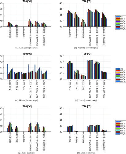
Figure 9. Treatment plans at 400 + 600 MHz for Alex. The SAR is normalized to the highest value in the patient. Transverse sections at target center. The target is delineated in white. The magenta/cyan voxels represent locations of highest/lowest SAR (hot-spot/cold-spot), excluding the first centimeter of tissue from the skin surface.

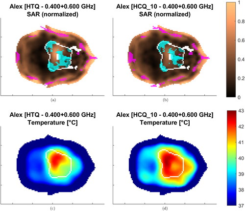
Figure 10. Treatment plans at 500 MHz for Venus. The SAR is normalized to the highest value in the patient. Sagittal sections at target center. The target is delineated in white. The magenta/cyan voxels represent locations of highest/lowest SAR (hot-spot/cold-spot), excluding the first centimeter of tissue from the skin surface.

The correlation coefficients between the inverse of the cost functions and the clinical indicators are summarized in Table 2. Values of cross-correlation between clinical indicators are also included. We report the values obtained for deep-seated targets, i.e., excluding the superficial case of Venus, and for the entire dataset (within parenthesis). In the first case, the HCQ evaluated at a low percentile (p ≤ 30%) exhibits a high correlation with both the target coverage indicators TC₅₀, TC₇₅ and the temperature indicators T₅₀, T₉₀. HTQ, on the other hand, is adequately correlated with TC₅₀, but the correlation deteriorates for other indicators, confirming that tumor coverage is not captured by this metric. The overall correlation is preserved for HTQ when the superficial case (Venus) is included, but the correlation of HCQ with the temperature indicators drops on average by 5 points with T₅₀ and by 8 points with T₉₀. Simultaneously, the optimal percentile shifts toward higher volume fractions, p≈50%. It is worth noting that the cross-correlation between SAR and temperature indicators also decreases substantially, loosing up to 31 points between TC₇₅ and T₉₀. To better visualize the relationships between cost functions and clinical indicators, Figures 11 and 12 display the dispersion plots and the fitted linear regression models for HTQ and HCQ₃₀.

Figure 11. Dispersion plots and linear regression models for the relationship between HTQ and the clinical indicators. Model fit on all treatment plan values excluding samples relative to Venus.

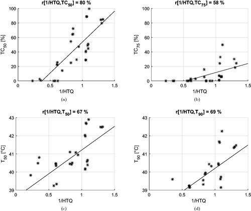
Figure 12. Dispersion plots and linear regression models for the relationship between HCQ₃₀ and the clinical indicators. Model fit on all treatment plan values excluding samples relative to Venus.

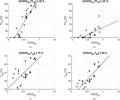
Table 2. Correlation coefficients between the inverse of the cost functions (HTQ, HCQ) and the clinical indicators (T, TC).

r [%]	TC 50	TC 75	T50	T90
1/HTQ	80 (82)	58 (55)	67 (70)	69 (73)
1/HCQ01	90 (91)	69 (80)	59 (49)	79 (61)
1/HCQ10	93 (94)	71 (76)	68 (58)	83 (65)
1/HCQ30	92 (93)	67 (68)	70 (62)	85 (72)
1/HCQ50	92 (93)	69 (68)	72 (67)	84 (76)
1/HCQ70	88 (89)	65 (64)	70 (67)	76 (73)
1/HCQ90	77 (78)	52 (54)	65 (66)	61 (62)
1/HCQ99	67 (68)	45 (47)	55 (57)	47 (50)
TC 50	−100−	70 (72)	70 (64)	81 (73)
TC 75	70 (72)	−100−	69 (43)	75 (44)
T50	70 (64)	69 (43)	−100−	93 (94)
T90	81 (73)	75 (44)	93 (94)	−100−

The main value is obtained excluding the results from Venus, while the value between parenthesis is obtained including the results from Venus. The best correlation coefficient for each indicator is highlghted in yellow. The last four rows report the cross-correlation between clinical indicators.

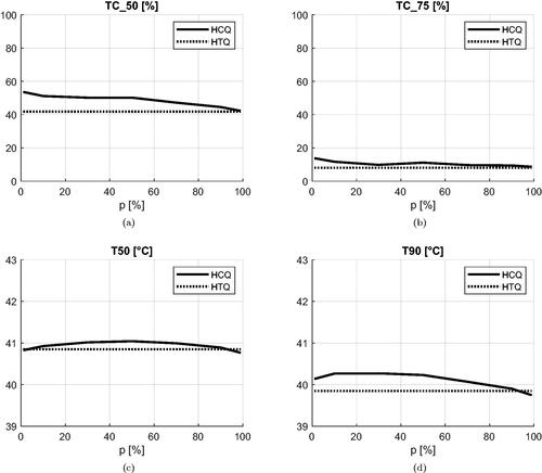
To address the question of the sensitivity of HCQ to the target percentile parameter, we report in Figure 13 the average values of the clinical indicators as a function of p. While the SAR indicators peak at p = 1%, the temperature indicators are maximized at larger percentiles. The optimal percentile for T₅₀ is p = 50%, while T₉₀ is highest at p = 10%, although high values are obtained up to p ≤ 50%. Overall, HCQ achieves higher SAR and temperature values than HTQ for most percentile settings.

Figure 13. Average value of each clinical indicator as a function of the HCQ target percentile parameter p (solid line). The average values relative to HTQ are also reported for comparison (dotted line). The average is taken across all treatment plans excluding samples relative to Venus.

4. Discussion

According to clinical evidence, treatment planning in HT therapy should always strive to achieve high temperatures everywhere in the target volume, as this is crucial for a successful outcome [48–50]. This requirement is represented by the clinical indicators T₅₀ and T₉₀. SAR-based optimization is a means to obtain the desired temperature distribution in the treated region, as shown for instance in [14,17,51], and temperature changes have been shown to accurately follow SAR-based steering during treatment [52].

Still, SAR is not temperature, and the relationship between local SAR and local temperature is not straightforward. Therefore, it is of paramount importance that the goal in SAR-based treatment planning translates to optimal values of temperature indicators. Numerous efforts have been spent in this regard, as summarized by [19]. To date, the routine in clinical SAR-based optimization is to minimize the HTQ, which has been shown to correlate with T₅₀ in pelvic tumors [14]. The relationship between 1/HTQ and the temperature indicators T₅₀ and T₉₀ has been further examined in head and neck carcinomas [27] and shown to be sub-optimal for many cases (≤ 60%). A possible explanation is the fact that HTQ considers the average SAR in the whole target volume, implicitly neglecting areas of low deposition (cold-spots). Another limitation of HTQ is the definition of the hot-spot as a percentile of healthy tissue, which makes the resulting value sensitive to volumetric changes in patient segmentation. A possible workaround is to keep the hot-spot sub-volume constant, for instance 50 ml as proposed in [31]. In Appendix A, we show that this is only a partial solution to the problem, which leads to both higher and lower correlation with the clinical indicators and lower absolute values in general. This might be due to HTQ not truly considering the actual target volume size. Furthermore, HTQ might not easily generalize to octave UWB optimizations where the size of the focal spot, and potentially even the size of the hot-spots, can vary double-fold.

To improve on this aspect, we have proposed the HCQ as a means to obtain high and homogeneous SAR deposition in the target, while limiting the most prominent hot-spot [29]. HCQ is a non-linear metric, since the identification of the hot-and cold-spots involves a percentile operation. Unlike quadratic metrics, the HCQ cannot be reduced to a direct function of the steering parameters only. Instead, the whole SAR distribution has to be screened upon each evaluation. This has the drawback of requiring iterative optimization procedures. On the other hand, this also enables the HCQ to better capture the requirements of a good HT treatment plan than quadratic measures. Previously, we observed that HCQ has the potential to extend SAR deposition in cold regions of the target. The current work, which benchmarks the performances of HCQ against a commonly used cost-function on a comprehensive set of patients, confirms this claim. In the deep seated targets, HCQ yields systematically higher values than HTQ in all clinical indicators. Moreover, in at least three cases (Alex, Murphy and Luna), the multi-frequency HCQ-optimal treatment plans increase the temperature indicators T₅₀ and T₉₀ by up to half a degree with respect to the best single-frequency or HTQ solutions. Despite the discrepancies between absolute temperature predictions by thermal simulations and clinically measured values [46], the gain is nevertheless relevant in view of the proven accuracy in predicted relative temperature changes [53].

The behavior of the multi-frequency plans, however, is not consistent. In a number of specific cases (for example, Alex HCQ₁₀ 400 MHz versus 400 + 800 MHz), the addition of a second frequency leads to lower absolute temperatures. Thus, while not conclusive, these results follow our previous findings that, in a multi-frequency setting, the HCQ-optimal solution can, but is not guaranteed to, achieve broader target coverage by exploiting complementary SAR deposition patterns [54]. A clear relationship between frequency set, patient anatomy, and temperature increase has yet to be uncovered. Due to the peculiar shape of the target volume in Alex, one could argue that the addition of a second frequency might be beneficial when the tumor is irregular, such as when it is composed of several mass centers. Of course, further studies are required to verify this, and to quantitatively assess the potential gain in temperature versus the additional costs and technical difficulties that must be overcome to clinically deploy a multi-frequency system. In particular, multi-frequency treatments require complex RF cascades that can either multiplex several frequencies into each channel, with independent phase and amplitude control for each frequency and channel, or finely interleave different operating modes in time [20,55].

We carried out the analysis on a patient repository prepared by ESHO, which is meant to be the first step toward the creation of a standard for the quantitative comparison of different HTP optimization strategies. The dataset is accompanied by a benchmark paper [31]. Presently, however, we do not aim for a direct comparison between the results reported here and those reported in the benchmark paper, because the differences between our methods are too broad to allow meaningful comparisons. Rather, we intend to provide a fair comparison between HTQ and HCQ when applied under the same conditions (applicator design, patient, target, SAR processing, optimization algorithm). Nevertheless, we include a discussion on potential differences for completeness.

In the reference paper [31], three patient models are devoted to SAR-based optimization, and another three are reserved to temperature-based optimization. To increase the statistical significance of our results, we carried out HTP optimizations for all six patients. Our thermal simulations result in slightly different tumor temperatures than those reported in [31], even when applying HTQ as cost function. There might be several reasons behind these deviations. The major difference lies in the applicator design. In our study, all patients are treated with tailored applicators based on more efficient antennas than the monopoles used in the benchmark. The arrays are assembled by maximizing the number of antennas with given constraints on the minimum distance between them, while the distance between each antenna and the patient is kept as close as possible to the optimum. This results in a higher number of antennas per applicator than in [31], except in the breast models. Thermal modeling can also be a factor. We applied a water bolus convection coefficient of 100 W/m[²/K], an average value in the range reported by [41] and previously adopted by [56]. The benchmark paper [31] recommends a maximum value of 40 [W/m²/K], with space for adjustments. However, it is not entirely clear whether this applies to the air/skin or the water/skin interface. Finally, we strictly followed the material properties reported in [33], while the benchmark paper applies adjustments for thermal stress (muscle, fat and breast) and custom baseline values for breast gland. In this study, however, we are interested in the correlation between HCQ and the HTP indicators, and therefore, we opted for a worst case scenario without perfusion enhancements.

This study indicates that HCQ is an effective metric for SAR-based treatment planning, providing high correlation with the temperature indicators for targets located deeply in the body, where the cooling effect of the water bolus is negligible. If the tumor is closer to the surface, the overall correlation between SAR and temperature degrades. This can be seen in the lower part of Table 2, where the cross-correlations between SAR and temperature indicators are reported. When the superficial case (Venus) is excluded, the correlation between TC and T is high (average r ≈ 74%). On the other hand, when the whole dataset is considered, the correlation drops severely (average r ≈ 56%). This degradation affects the HCQ-based plan for Venus, where it performs worse compared to HTQ. Although one case is not statistically significant for a general conclusion, it is possible to identify a rationale behind this specific result by visual inspection of the SAR and temperature distributions (Figure 10). In SAR, the main hot-spot of the HTQ-optimal solution lies in the layer of healthy tissue between the tumor and the water bolus. Normally, this deposition peak would limit the maximum power to the tumor, which in turn would result in poor coverage of its deeper parts. However, due to the cooling effect of the water bolus, the hot-spot is efficiently suppressed, leading to preferential power absorption and thus high temperatures in the tumor. The HCQ-optimal solution, conversely, extends the SAR deposition deeper in the target. As a consequence, the main deposition peak arises on the proximal side of the tumor. This hot-spot, however, is not counterbalanced by cooling, and becomes the limiting factor in the power scaling. It is known that the water bolus has a direct effect on the temperature distribution up to a couple of centimeters from the skin surface, a behavior that has been thoroughly characterized as depending on the water temperature and the quality of the contact at the skin/bolus interface [41]. If part of the target volume lies in this superficial layer, as is the case for Venus, the bolus itself becomes a heat source (or sink) to be considered in the treatment plan. In such cases, temperature-based optimization strategies might be more appropriate, as they can account for the heat extraction of the bolus via boundary conditions. The temperature of the water bolus itself can even be included in the vector of optimization parameters to achieve the desired temperature of 43 °C everywhere in the target [57]. Of course, this mechanism needs to be verified on a broader set of superficial tumors.

Although the choice of an appropriate cost function is crucial to achieve an adequate SAR-based treatment plan, other parameters play an important role as well. In fact, the SAR optimization relies on the assumption that the SAR and temperature distributions are spatially correlated. For this to be true, the raw SAR distribution must be treated with a smoothing filter. This problem has been thoroughly addressed in the literature [58–60], resulting in number of proposed averaging schemes. In our investigations, we have identified the 1 g tissue mass scheme as most suitable for our purposes. Concurrently, the correlation of SAR and temperature can be further enhanced by the exclusion of the first centimeter of tissue that is in contact with the water bolus [41]. Only under these conditions can the HCQ achieve high correlation with the temperature indicators. The strength of this relationship can also be inferred from Figure 13, where the peak T₅₀ is obtained for the 50-percentile HCQ, while the peak T₉₀ is achieved for the 100 − 90 = 10-percentile HCQ. Note that the exclusion of SAR regions from the evaluation of the HCQ does not prevent the enforcement of local SAR exposure limits for safety reasons [61,62]. Constrained global optimization algorithms can be utilized to solve for the HCQ in this case [63], by evaluating the constraint over the whole SAR distribution.

5. Conclusion

This work validates the HCQ as goal for SAR-based treatment planning on a heterogeneous patient repository. The HCQ-based optimization yields high tumor temperatures and exhibits high correlation with clinical SAR and temperature indicators. This correlation is a result of the metric definition, along with careful pre-processing of the SAR distribution. The results indicate that HCQ-optimal treatment plans can achieve higher and more homogeneous temperatures in the target than plans based on current SAR approaches. In a few cases, the use of HCQ as cost function promotes the exploitation of additional operating frequencies to increase target coverage. The use of multiple frequencies can improve a plan in specific instances, but the benefit is not consistent and has to be characterized in future studies. The validation performed on a set of six patient models that cover some of the most common HT treatment sites demonstrates that HCQ is a powerful and robust goal in HTP optimization, provided the target is located far from the range of effect of the water bolus. For superficial targets, the correlation between SAR and temperature is degraded, and temperature-based treatment planning optimization strategies might prove more suitable.

Disclosure statement

No potential conflict of interest was reported by the authors.

Additional information

Funding

This work was supported by Vetenskapsrådet [No. 2021-04935].

Appendix A. Results for HTQ with fixed 50 ml hot-spot size

We report here the results relative to the treatment plans obtained using the following modified definition of HTQ with a fixed hot-spot size [27,31]: (8) $${\text{HTQ}}^{’}\text{=}\frac{{\overline{\mathrm{SAR}}}_{\mathrm{R}50}}{{\overline{\mathrm{SAR}}}_{\mathrm{T}}}$$(8) where R₅₀ is the 50 ml sub-volume of remaining tissue with the highest SAR values. The overall results are shown as scatter plots in Figure A1. These can be compared to Figure 11 where the traditional definition of HTQ (Eq. 3(3) $$\mathrm{HTQ}=\frac{{\overline{\text{SAR}}}_{\mathrm{R}1}}{{\overline{\text{SAR}}}_{\mathrm{T}}}$$(3) ) has been used. The correlation with the SAR indicators TC is lower (7.5 points on average), while the correlation with the temperature indicators T is remarkably higher (21 points on average). However, the absolute index values do not improve, but rather worsen. The SAR indicator TC₅₀ for the HTQ’-optimal plans (excluding Venus) becomes 37% on average (compare 48% for HTQ and 58% for HCQ₃₀), while TC₇₅ becomes 5% on average (compare 11% for HTQ and 20% for HCQ₃₀). The average T₅₀ is 40.8 °C (compare 41.0 °C for HTQ and 41.0 °C for HCQ₃₀), while the average T₉₀ is 39.8 °C (compare 40.0 °C for HTQ and 40.2 °C for HCQ₃₀). In the specific case of Venus, the temperatures drop remarkably with respect to the plans based on the classic HTQ. These are reported in Figure A2, to be compared with the blue bars in Figures 7(d) and 8(d). The T values for HTQ’ are almost half a degree lower than their HTQ counterparts. While not conclusive, these results suggest that the modification (8) does not address the fundamental limitation of HTQ in modeling the target coverage as effectively as HCQ. While HTQ’ exhibits a slightly higher (relative) correlation with the temperature indexes than HCQ, we believe the latter is still preferable as it consistently leads to higher absolute values, especially in the cold-spots.

Figure A1. Dispersion plots and linear regression models for the relationship between HTQ^′ and the clinical indicators. Model fit on all treatment plan values excluding samples relative to Venus.

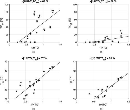
Figure A2. Treatment plan values of T₅₀ and T₉₀ obtained using HTQ^′ for Venus at each frequency combination.

References

- Kok HP, Cressman EN, Ceelen W, et al. Heating technology for malignant tumors: a review. Int J Hyperthermia. 2020;37(1):711–741.
- Paulides M, Trefna HD, Curto S, et al. Recent technological advancements in radiofrequency-andmicrowave-mediated hyperthermia for enhancing drug delivery. Adv Drug Delivery Rev. 2020;163–164:3–18.
- Elming PB, Sørensen BS, Oei AL, et al. Hyperthermia: the optimal treatment to overcome radiation resistant hypoxia. Cancers. 2019;11(1):60.
- Issels RD, Lindner LH, Verweij J, et al. Effect of neoadjuvant chemotherapy plus regional hyperthermia on long-term outcomes among patients with localized high-risk soft tissue sarcoma: the EORTC 62961-ESHO 95 randomized clinical trial. JAMA Oncol. 2018;4(4):483–492.
- Datta N, Ord´õnez SG, Gaipl U, et al. Local hyperthermia combined with radiotherapy and-/or chemotherapy: recent advances and promises for the future. Cancer Treat Rev. 2015;41(9):742–753.
- Yarmolenko PS, Moon EJ, Landon C, et al. Thresholds for thermal damage to normal tissues: an update. Int J Hyperthermia. 2011;27(4):320–343.
- Sapareto SA, Dewey WC. Thermal dose determination in cancer therapy. Int J Radiat Oncol Biol Phys. 1984;10(6):787–800.
- Bruggmoser G, Bauchowitz S, Canters R, et al. Quality assurance for clinical studies in regional deep hyperthermia. Strahlenther Onkol. 2011;187(10):605–610.
- Kok H, Wust P, Stauffer PR, et al. Current state of the art of regional hyperthermia treatment planning: a review. Radiat Oncol. 2015;10(1):1–14.
- Kok H, Crezee J. Progress and future directions in hyperthermia treatment planning. In: 2017 First IEEE MTT-S International Microwave Bio Conference (IMBIOC). IEEE, Piscataway (NJ). 2017. p. 1–4.
- Gavazzi S, van Lier AL, Zachiu C, et al. Advanced patient-specific hyper-thermia treatment planning. Int J Hyperthermia. 2020;37(1):992–1007.
- Kok H, Kotte A, Crezee J. Planning, optimisation and evaluation of hyperthermia treatments. Int J Hyperthermia. 2017;33(6):593–607.
- Schooneveldt G, Dobšíček Trefná H, Persson M, et al. Hyperthermia treatment planning including convective flow in cerebrospinal fluid for brain tumour hyperthermia treatment using a novel dedicated paediatric brain applicator. Cancers. 2019;11(8):1183.
- Canters R, Franckena M, van der Zee J, et al. Optimizing deep hyperthermia treatments: are locations of patient pain complaints correlated with modelled SAR peak locations? Phys Med Biol. 2011;56(2):439–451.
- Lee HK, Antell AG, Perez CA, et al. Superficial hyperthermia and irradiation for recurrent breast carcinoma of the chest wall: prognostic factors in 196 tumors. Int J Radiat Oncol Biol Phys. 1998;40(2):365–375.
- Kok HP, Korshuize-van Straten L, Bakker A, et al. Online adaptive hyperthermia treatment planning during locoregional heating to suppress treatment-limiting hot spots. Int J Radiat Oncol Biol Phys. 2017;99(4):1039–1047.
- Rijnen Z, Bakker JF, Canters RA, et al. Clinical integration of software tool VEDO for adaptive and quantitative application of phased array hyperthermia in the head and neck. Int J Hyperthermia. 2013;29(3):181–193.
- Shoji H, Motegi M, Osawa K, et al. Output-limiting symptoms induced by radiofrequency hyperthermia. Are they predictable? Int J Hyperthermia. 2016;32(2):199–203.
- Canters R, Wust P, Bakker J, et al. A literature survey on indicators for characterisation and optimisation of SAR distributions in deep hyperthermia, a plea for standardisation. Int J Hyperthermia. 2009;25(7):593–608.
- Kuehne A, Oberacker E, Waiczies H, et al. Solving the time-and frequency-multiplexed problem of constrained radiofrequency induced hyperthermia. Cancers. 2020;12(5):1072.
- Bellizzi GG, Drizdal T, van Rhoon GC, et al. The potential of constrained SAR focusing for hyperthermia treatment planning: analysis for the head & neck region. Phys Med Biol. 2018;64(1):015013.
- Mestrom R, Van Engelen J, Van Beurden M, et al. A refined eigenvalue-based optimiza-tion technique for hyperthermia treatment planning. In: The 8th European Conference on Antennas and Propagation (EuCAP 2014). IEEE, Piscataway (NJ). 2014. p. 2010–2013.
- K¨ohler T, Maass P, Wust P, et al. A fast algorithm to find optimal controls of multiantenna applicators in regional hyperthermia. Phys. Med. Biol. 2001;46(9):2503–2514.
- Zanoli M, Trefn´a HD. Suitability of eigenvalue beam-forming for discrete multi-frequency hyperthermia treatment planning. Med Phys. 2021;48(11):7410–7426.
- Canters R, Franckena M, Paulides M, et al. Patient positioning in deep hyperthermia: influences of inaccu-racies, signal correction possibilities and optimization potential. Phys Med Biol. 2009;54(12):3923–3936.
- Sherar M, Liu FF, Pintilie M, et al. Relationship between thermal dose and outcome in thermoradiotherapy treatments for superficial recurrences of breast cancer: data from a phase III trial. Int J Radiat Oncol Biol Phys. 1997;39(2):371–380.
- Bellizzi GG, Drizdal T, van Rhoon GC, et al. Predictive value of SAR based quality indicators for head and neck hyperthermia treatment quality. Int J Hyperthermia. 2019;36(1):455–464.
- Triantopoulou S, Efstathopoulos E, Platoni K, et al. Radiotherapy in conjunction with superficial and intracavitary hyperthermia for the treatment of solid tumors: survival and thermal parameters. Clin Transl Oncol. 2013;15(2):95–105.
- Zanoli M, Trefn´a HD. Combining target coverage and hot-spot suppression into one cost function: the hot-to-cold spot quotient. In: 2021 15th European Conference on Antennas and Propagation (EuCAP). IEEE, Piscataway (NJ). 2021. p. 1–4.
- Bellizzi GG, Sumser K, VilasBoas-Ribeiro I, et al. Standardization of patient modeling in hyperthermia simulation studies: introducing the erasmus virtual patient repository. Int J Hyperthermia. 2020;37(1):608–616.
- Paulides MM, Rodrigues DB, Bellizzi GG, et al. ESHO benchmarks for computational modeling and optimization in hyperthermia therapy. Int J Hyperthermia. 2021;38(1):1425–1442.
- James BJ, Sullivan DM. Creation of three-dimensional patient models for hyperthermia treatment planning. IEEE Trans Biomed Eng. 1992;39(3):238–242.
- Hasgall PA, Di Gennaro F, Baumgartner C, et al. IT’IS Database for thermal and electromagnetic parameters of biological tissues. Version 4.1. DOI:10.13099/VIP21000-04-1 Itis.swiss/database. 2018.
- Joines WT, Zhang Y, Li C, et al. The measured electrical properties of normal and malignant human tissues from 50 to 900 MHz. Med Phys. 1994;21(4):547–550.
- Takook P, Persson M, Gellermann J, et al. Compact self-grounded Bow-Tie antenna design for an UWB phased-array hyperthermia applicator. Int J Hyperthermia. 2017;33(4):387–400.
- Seebass M, Beck R, Gellermann J, et al. Electromagnetic phased arrays for regional hyperthermia: optimal frequency and antenna arrangement. Int J Hyperthermia. 2001;17(4):321–336.
- Paulides MM, Vossen SH, Zwamborn AP, et al. Theoretical investigation into the feasibility to deposit RF energy centrally in the head-and-neck region. Int J Radiat Oncol Biol Phys. 2005;63(2):634–642.
- Kok H, De Greef M, Borsboom P, et al. Improved power steering with double and triple ring waveguide systems: the impact of the operating frequency. Int J Hyperthermia. 2011;27(3):224–239.
- COMSOL AB, Stockholm, Sweden. COMSOL Multiphysics® v. 5.6 11. 2020.
- The MathWorks Inc, Natick, Massachusetts. MATLAB R2021. 2021.
- Van der Gaag M, De Bruijne M, Samaras T, et al. Development of a guideline for the water bolus temperature in superficial hyperthermia. Int J Hyperthermia. 2006;22(8):637–656.
- Clerc M. Particle swarm optimization. Vol. 93. Hoboken (NJ): John Wiley & Sons; 2010.
- Pedersen MEH. Good parameters for particle swarm optimization. Tech Rep HL1001. Copenhagen, Denmark: Hvass Lab; 2010. p. 1551–3203.
- Liu X, Chen S, Tsoi JK, et al. Binary titanium alloys as dental implant materials - a review. Regen Biomater. 2017;4(5):315–323.
- Verhaart RF, Verduijn GM, Fortunati V, et al. Accurate 3D tempera-ture dosimetry during hyperthermia therapy by combining invasive measurements and patient-specific simulations. Int J Hyperthermia. 2015;31(6):686–692.
- Aklan B, Zilles B, Paprottka P, et al. Regional deep hyperthermia: quantitative evaluation of predicted and direct measured temperature distributions in patients with high-risk extremity soft-tissue sarcoma. Int J Hyperthermia. 2019;36(1):169–184.
- Bakker A, van der Zee J, van Tienhoven G, et al. Temperature and thermal dose during radiotherapy and hyperthermia for recurrent breast cancer are related to clinical outcome and thermal toxicity: a systematic review. Int J Hyperthermia. 2019;36(1):1023–1038.
- Refaat T, Sachdev S, Sathiaseelan V, et al. Hyperthermia and radiation therapy for locally advanced or recurrent breast cancer. Breast. 2015;24(4):418–425.
- Franckena M, Fatehi D, de Bruijne M, et al. Hyperthermia dose-effect relationship in 420 patients with cervical cancer treated with combined radiotherapy and hyperthermia. Eur J Cancer. 2009;45(11):1969–1978.
- Jones EL, Oleson JR, Prosnitz LR, et al. Randomized trial of hyperthermia and radiation for superficial tumors. J Clin Oncol. 2005;23(13):3079–3085.
- Verduijn G, de Wee E, Rijnen Z, et al. Deep hyperthermia with the HYPERcollar system combined with irradiation for advanced head and neck carcinoma–a feasibility study. Int J Hyperthermia. 2018;34(7):994–1001.
- Kok HP, Ciampa S, de Kroon-Oldenhof R, et al. Toward online adaptive hyperthermia treatment planning: correlation between measured and simulated specific absorption rate changes caused by phase steering in patients. Int J Radiat Oncol Biol Phys. 2014;90(2):438–445.
- Kok H, Schooneveldt G, Bakker A, et al. Predictive value of simulated SAR and temperature for changes in measured temperature after phase-amplitude steering during locoregional hyperthermia treatments. Int J Hyperthermia. 2018;35(1):330–339.
- Zanoli M, Trefn´a HD. Iterative time-reversal for multi-frequency hyperthermia. Phys Med Biol. 2021;66(4):045027.
- Trefn´a HD, Martinsson B, Petersson T, et al. Multifrequency approach in hyperthermia treatment planning: impact of frequency on SAR distribution in head and neck. In: 2017 11th European Conference on Antennas and Propagation (EUCAP). IEEE, Piscataway (NJ). 2017. p. 3710–3712.
- Kumaradas J, Sherar M. Edge-element based finite element analysis of microwave hyperthermia treatments for superficial tumours on the chest wall. Int J Hyperthermia. 2003;19(4):414–430.
- Dobšíček Trefná H, Crezee J, Schmidt M, et al. Quality assurance guidelines for superficial hyperthermia clinical trials. Strahlenther Onkol. 2017;193(5):351–366.
- Razmadze A, Shoshiashvili L, Kakulia D, et al. Influence of specific absorption rate averaging schemes on correlation between mass-averaged specific absorption rate and temperature rise. Electromag-netics. 2009;29(1):77–90.
- Hirata A, Fujiwara O. The correlation between mass-averaged SAR and temperature elevation in the human head model exposed to RF near-fields from 1 to 6 GHz. Phys Med Biol. 2009;54(23):7227–7238.
- Bakker J, Paulides M, Neufeld E, et al. Children and adults exposed to electromagnetic fields at the ICNIRP reference levels: theoretical assessment of the induced peak temperature increase. Phys Med Biol. 2011;56(15):4967–4989.
- IEEE recommended practice for determining the peak spatial-average specific absorption rate (SAR) in the human head from wireless communications devices: measurement techniques. IEEE Std. 1528;2013:1–246.
- Kroesen M, van Holthe N, Sumser K, et al. Feasibility, SAR distribution, and clinical outcome upon reirradiation and deep hyperthermia using the hypercollar3D in head and neck cancer patients. Cancers. 2021;13(23):6149.
- Venter G. Review of optimization techniques. In: Blockley R, Shyy W, editors. Encyclopedia of Aerospace Engineering. John Wiley & Sons; 2010. DOI:10.1002/9780470686652.eae495