Bayesian change-point modelling of the effects of 3-points-for-a-win rule in football

ABSTRACT

We examine the effects of the 3-points-for-a-win (3pfaw) rule in the football world. Data that form the basis of our analyses come from seven leagues around the world (Albania, Brazil, England, Germany, Poland, Romania, and Scotland) and consist of mean goals and proportions of decided matches over a period of about six years before- and about seven years after the introduction of the rule in the respective leagues. Bayesian change-point analyses and Shiryaev-Roberts tests show that the rule had no effects on the mean goals but, indeed, had increasing effects on the proportions of decided matches in most of the leagues studied. This, in turn, implies that while the rule has given teams the incentive to aim at winning matches, such aim was not achieved by scoring excess goals. Instead, it was achieved by scoring enough goals in order to win and, at the same time, defending enough in order not to lose. Our results are in accordance with recent findings on comparing the values of attack and defense - that, in top-level football, not conceding a goal is more valuable than scoring a single goal.

KEYWORDS:

• Bayesian inference
• Bayes factor
• change-point models
• excitement index
• football
• Shiryaev–Roberts change point detection scheme
• three-points-for-a-win rule

2010 MATHEMATICS SUBJECT CLASSIFICATION:

• 62F15

1. Introduction

1.1. Background

Prior to 1981, the point-awarding system in football (soccer) was 2 points for a win, 1 point for a draw, and 0 point for a loss. A 3-points for a win (3pfaw) system was introduced first in England in 1981 with the aim to provide teams with incentive to aim at winning games. This, in turn, was expected to lead to more offensive and, hence, more exciting football that would increase public attendance.

According to Anderson and Sally [1], the 3pfaw rule is the legacy of Jimmy Hill (1928–2015) who ‘had long thought that football had become too defensive and dull, too uninteresting for spectators’. He felt that goals had become rarer with every passing season and, hence, change was needed for professional football to thrive. Hill's far-reaching proposal was that ‘victory should be rewarded with three points, rather than two, to make wins more valuable’. After a trial in the 1970s, the Football Association (FA) in England was convinced of Hill's idea and implemented it in 1981. Since the experiment in England was judged as success, FIFA followed it in 1995 and commanded member countries to award three points for a victory. The then general secretary of FIFA, Sepp Blatter, is cited in Anderson and Sally [1] labelling the rule as the most important decision taken by FIFA in rewarding attacking soccer where the reward was 50 per cent greater. The expected result was, thus, encouraging teams to take risks leading to more goals which, in turn, leads to more entertainment and more spectators. Finding out whether the change worked as intended calls for more accurate methodological procedures and this is the main goal of the present paper.

The above-mentioned objective of the 3pfaw system, encouraging teams to aim at winning matches, was expected to be reflected in either increased number of goals per match, increased number of decided matches (decreased draws), or both.

Some researchers have attempted to measure the effect of the reform in various ways and with diverging results. For instance, Brocas and Carrillo [4] analyse the dynamics of the game strategies of teams using game theory and observe that, under the 3pfaw rule, teams tend to play more defensively rather than playing offensive football. Dilger and Geyer [7], on the other hand, apply regression model on data from the German league and conclude that the introduction of the 3pfaw rule has significantly increased the mean goals as well as the proportion of decided matches. Such observation is supported by Moschini [15] who uses a game-theoretic model to investigate the effects of the 3pfaw rules in 35 different countries and concludes that the rule has led to statistically significant increase in the number of expected goals and decrease in the number of drawn matches. In contrast, Hon and Parinduri [12] use regression discontinuity design on data from the German league and find no evidence that 3pfaw makes the games more decisive, increases the number of goals, or decreases goal differences. Skinner and Freeman [21] use Bayesian methods to determine how often the team with greater ability actually wins a football match. Anderson and Sally's [1] analyse various aspects of football games from top-levels leagues. One of their main findings is that it is statistically more valuable to prevent a goal than to score one.

1.2. Excitement index approach

Aylott and Aylott [2] define an Excitement Index (EI) by combining points allocated to decided matches and to each goal scored. A decided match is allocated 1 point while a match that ends in a draw is allocated 0 point. Further, each goal scored in a match is allocated 0.2 points and the EI for each year and country is computed as a sum of these points. The allocation of points to decided matches and scored goals is in accordance with the intended aim of the 3pfaw rule (increase the proportion of decided matches and the number of goals). They then plot the EI-values for each of the seven leagues and years (from about 6 years before and about 7 years after the 3pfaw rule). Based on the trends in the EI for each league (and another plot of aggregated effect of the 3pfaw on EI in all seven leagues), Aylott and Aylott [2] conclude that there was an increase in excitement after the introduction of 3pfaw rule but that it took some years for the rule to take full effect.

A drawback in the above approach is that no formal test is made to see if the differences between the Excitement Indexes before and after the introduction of the 3pfaw are statistically significant. Moreover, the definition of Excitement Index is in itself questionable and subjective. For instance, a match that ends with 3-0 win for the home-team will have an Excitement Index of 1.6 but a match that ends with 0-3 win for the away-team or even in a 4-4 draw will also have the same value (EI=1.6). Yet, it is hard to conclude that these three matches are equally exciting as this is subjective and depends on the observer's ‘taste’, whether she or he is a neutral observer or supports the home- or away-team, etc.

1.3. The current study

The drawback outlined above calls for a statistically well grounded, theoretically appropriate, and empirically evident alternative to measure the effects of the 3pfaw rule. In the present paper, we use Bayesian change-point modelling [18] to re-analyse the data in [2]. We use Bayes Factors, posterior probabilities, and Shiryaev-Roberts test statistics [19,20,24,25], as evidence in support for or against a no-change model. Our empirical results do not lend support to changes in the mean goals after the introduction of the 3pfaw rule in any of the leagues studied. On the other hand, we find strong evidence for increase in the proportions of decided matches after the 3pfaw rule in at least five of the seven leagues studied. Further, our results show that the effects of the 3pfaw rule on the proportion of decided matches was immediate in some of the leagues and did not take long time to take full effect. This, in turn, implies that the 3pfaw rule has encouraged teams to aim more at winning matches (even marginally) than at scoring excess goals. In other words, the 3pfaw rule which was expected to make football more offensive has, in fact, made it both offensive and defensive.

In Section 2, we introduce the data sets and provide results from preliminary analyses using standard statistical methods. In Section 3, we describe the Bayesian change-point model in general and how it can be applied to the data sets at hand. Section 4 presents empirical findings from fitting the Bayesian change-point model to mean goals and proportions of decided matches. In Section 5, we compare our approach with the Shiryaev–Roberts test statistics which is common in the change point detection literature. Section 6 summarises the findings of the paper by way of concluding remarks and suggestions for future work.

2. The data sets

The data sets that form the basis for this study come from seven leagues around the world - Albania, Brazil, England, Germany, Poland, Romania, and Scotland where the 3pfaw rule was introduced in 1996, 1994, 1981, 1995, 1995, 1994, and 1994, respectively [2]. The data for each league contains information on the number of games, mean goals per game, and proportion of decided matches in each of the six years before introduction of the 3pfaw rule and seven years after the introduction of the rule. According to Aylott and Aylott [2], these seven leagues were maximally heterogeneous in different aspects like geographic location, history, wealth, country size, population size, and the time of introduction of the 3pfaw rule and were selected in order to avoid or minimise any kind of correlations across the selected cases.

We begin our analyses by conducting t-tests for equality between mean goals before and after the 3pfaw and, separately, tests of association between period (before or after the 3pfaw rule) and match-outcomes (drawn or decided). The relevant data are obtained by aggregating data from the 6 years before the 3pfaw rule and those from seven years after the 3pfaw rule.

2.1. Mean goals per match

Table 1 contains mean goals from the seven leagues under study over a period of about 6 years prior to the introduction of the 3pfaw (indicated by ‘−’ in the first column) and about 7 years after (indicated by ‘+’ in the first column). See also Figure A1 in the Appendix for a plot of the mean goals.

Table 1. Mean goals in 7 football leagues within about 6 years before and about 7 years after the introduction of the 3pfaw rule.

Years	Albania	Brazil	England	Germany	Poland	Romania	Scotland
$-5.5$	2.42	2.01	2.57	2.79	2.02	3.21	2.69
$-4.5$	2.63	1.89	2.64	2.62	2.41	2.92	2.73
$-3.5$	2.42	2.21	2.60	2.58	2.22	2.76	2.67
$-2.5$	2.27	2.29	2.56	2.62	2.61	2.49	2.71
$-1.5$	2.26	2.53	2.57	2.54	2.34	2.63	2.80
$-0.5$	2.19	2.40	2.47	2.63	2.40	2.44	2.51
$+0.5$	2.23	2.50	2.60	2.70	2.53	2.94	2.65
$+1.5$	2.28	2.72	2.77	2.64	2.50	2.63	2.69
$+2.5$	2.56	2.78	2.75	2.61	2.39	2.85	2.71
$+3.5$	2.58	2.88	2.72	2.61	2.53	2.91	2.80
$+4.5$	2.80	2.78	2.80	2.76	2.81	2.90	2.74
$+5.5$	2.81	2.89	2.60	2.86	2.56	2.98	2.81
$+6.5$	3.04	2.86	2.62	3.02	2.51	2.61	2.71

Source: Aylott and Aylott [2].

In Table 2 we present results from t-tests for equality of population means across the seven leagues.

Table 2. Results from tests of equality between mean goals before and after the 3pfaw.

	Albania	Brazil	England	Germany	Poland	Romania	Scotland
Mean (before)	2.37	2.22	2.58	2.62	2.32	2.73	2.68
Mean (after)	2.61	2.79	2.69	2.75	2.54	2.83	2.73
Var (before)	0.02	0.05	0.002	0.01	0.04	0.09	0.01
Var (after)	0.08	0.02	0.008	0.026	0.016	0.026	0.002
T-values	1.94	3.28	2.35	1.72	2.28	0.84	1.19
T(0.025;11)	2.20	2.20	2.20	2.20	2.20	2.20	2.20
T(0.05;11)	1.80	1.80	1.80	1.80	1.80	1.80	1.80

The results indicate that a two-sided test at 5% level shows significant differences between the mean goals for Brazil, England, and Poland. In a one-sided test at 5% level of significance (with the prior expectation that the rule increases mean goals), even Albania shows significant differences between mean goals (in addition to Brazil, England, and Poland). The above results provide some general picture of the phenomenon under investigation. However, it is to be recalled that they are obtained by aggregating the mean goals over the 6 years before the 3pfaw rule and comparing it with another mean that is obtained by aggregating the mean goals over the seven years after the 3pfaw rule.

2.2. Proportions of decided matches

Table 3 contains proportions of decided matches from the seven leagues under study over the same period as for the mean goals in the previous sub-section (see also Figure A2 in the Appendix).

Table 3. Proportions of decided matches in 7 football leagues within about 6 years before and 7 years after the 3pfaw rule.

Years	Albania	Brazil	England	Germany	Poland	Romania	Scotland
$-5.5$	0.749	0.662	0.723	0.697	0.625	0.863	0.712
$-4.5$	0.777	0.637	0.721	0.676	0.679	0.830	0.707
$-3.5$	0.774	0.648	0.691	0.656	0.644	0.797	0.734
$-2.5$	0.725	0.690	0.704	0.700	0.724	0.778	0.737
$-1.5$	0.723	0.705	0.721	0.704	0.654	0.784	0.740
$-0.5$	0.788	0.719	0.720	0.683	0.654	0.791	0.689
$+0.5$	0.761	0.732	0.726	0.703	0.745	0.817	0.739
$+1.5$	0.834	0.786	0.737	0.717	0.742	0.850	0.744
$+2.5$	0.850	0.695	0.740	0.686	0.742	0.824	0.744
$+3.5$	0.821	0.743	0.757	0.699	0.750	0.837	0.738
$+4.5$	0.794	0.775	0.754	0.706	0.738	0.843	0.761
$+5.5$	0.862	0.743	0.726	0.719	0.771	0.853	0.751
$+6.5$	0.809	0.770	0.727	0.757	0.714	0.754	0.747

Source: Aylott and Aylott [2].

In Table 4 we present results from tests for association between period (before or after the rule) and match-outcomes (drawn or decided). The frequencies are obtained by adding corresponding values in Table 2 of Aylott and Aylott [2] over the years before the 3pfaw rule and those after the rule. The results in Table 4 show that there are strong associations between the periods and the match-outcomes. This is true for all the leagues except Romania where the p-value associated with the ${\chi }^2$ (Chi-square) is 0.10 though even the p-value for the ${\chi }^2$ for Germany is also not as small as for the other countries.

Table 4. Results from tests of associations between the 3pfaw rule and match outcomes.

	Albania
	Drawn	Decided	Total	% decided	${\chi }^2$
Before	$580$	$1837$	$2417$	$76$
After	$432$	$1965$	$2397$	$82$	$25.87$ $(p=0.000)$
Total	$1012$	$3802$	$4814$	$79$
	Brazil
	Drawn	Decided	Total	% decided	${\chi }^2$
Before	$438$	$937$	$1375$	$68$
After	$519$	$1543$	$2062$	$75$	$18.35$ $(p=0.000)$
Total	$957$	$2480$	$3437$	$72$
	England
	Drawn	Decided	Total	% decided	${\chi }^2$
Before	$3488$	$8680$	$12168$	$71$
After	$3718$	$10480$	$14198$	$74$	$20.27(p=0.000)$
Total	$6720$	19160	26366	73
	Germany
	Drawn	Decided	Total	% decided	${\chi }^2$
Before	$1367$	$3011$	$4378$	$69$
After	$1232$	$3052$	$4284$	$71$	$6.27$ $(p=0.012)$
Total	$2599$	$6063$	8662	70
	Poland
	Drawn	Decided	Total	% decided	${\chi }^2$
Before	$572$	$1130$	$1702$	66
After	$482$	$1396$	$1878$	$74$	$27.11$ $(p=0.000)$
Total	$1054$	$2526$	$3580$	$71$
	Romania
	Drawn	Decided	Total	% decided	${\chi }^2$
Before	$354$	$1482$	$1836$	$81$
After	$558$	$1718$	$2076$	$83$	$2.70$ $(p=0.100)$
Total	$712$	$3200$	$3912$	$82$
	Scotland
	Drawn	Decided	Total	% decided	${\chi }^2$
Before	$1283$	$3298$	$4581$	$72$
After	$1291$	$3797$	$5088$	$75$	$8.56$ $(p=0.003)$
Total	$2574$	$7095$	$9669$	$73$

3. Bayesian change-point models

A change-point model assumes that a sequence of random variables $y_1,\dots ,y_T$ follows a distribution F before a change-point, say k, and follows another distribution G after the change-point [22]. The distributions F and G need not be the same and they may be known or unknown.

The change-point parameter, k, is unknown and is assumed to take on values in the set $\varkappa =\{1,2,\dots ,T\}$ where T is the length of the observation period. Evidence about whether a change occurred during the period of study is provided by testing a null hypothesis $H_0:k=T$ (no change) against $H_0:k<T$.

Change-point models have been applied in different areas like economics [26] and cognitive science [8,11]. Raftery and Akman [18] derive the posterior for the change-point model in Poisson process and use Bayes Factors to compare this model with a model that assumes a constant rate. Carlin et al. [5] develop Bayesian hierarchical models for change-point problems while Smith [22] considers cases of the change-point in the binomial and normal distributions. Lee [14] investigates, in a Bayesian framework, change-points in exponential family of distributions. Carlin et al. [5] and Chin Choy and Broemeling [6] study the problem of a single change-point in linear models using the Bayesian framework while Bauwens and Rombouts [3] and Van den Hout et al. [23] study a more general case of multiple change-points in linear models. Petrone and Raftery [16] investigate change point problems using a non-parametric Bayesian approach.

Despite the abundance of literature in the area of change-point models no previous study (to the best of our knowledge) has applied change-point modelling to assess the effect of the 3pfaw rule. In the next two sub-sections we apply Bayesian change-point modelling to analyse the mean goals and the proportions of decided matches in the data previously analysed by Aylott and Aylott [2].

3.1. Bayesian change-point model for mean goals

We consider the case where F and G are known and our interest is in inference about the parameters in the models as well as testing whether a change-point model is adequate for the data at hand. We assume that the mean goals per match, Y , follow a normal distribution with mean ${\mu }_1$ and variance ${\sigma }_1^2$ until the kth year. After the kth year, the mean goals per match follow a normal distribution with mean ${\mu }_2$ and variance ${\sigma }_2^2$ : (1) $\begin{array}{rl}{\mathbf{Y}}_t& \sim N\left({\mu }_1,{\sigma }_1^2\right),t=1,\dots ,k\\ {\mathbf{Y}}_t& \sim N\left({\mu }_2,{\sigma }_2^2\right),t=k+1,\dots ,T.\end{array}$(1) Further, following Gill [10], we assume Inverse gamma (IG) conjugate prior for the variances and conjugate normal prior for the means (which, in turn, are conditional on the variances): (2) $\begin{array}{rl}& p\left({\sigma }_j^2|{\alpha }_j,{\beta }_j\right)\propto {\left({\sigma }_j^2\right)}^{-\left({\alpha }_j-1\right)}\exp \left(-\frac{1}{{\sigma }_j^2}{\beta }_j\right),j=1,2\end{array}$(2) (3) $\begin{array}{rl}& p\left({\mu }_j|{\sigma }_j^2/s_j,m_j\right)\propto {\left({\sigma }_j^2\right)}^{-\left(1/2\right)}\exp \left(-\frac{1}{2{\sigma }_j^2/s_j}{\left({\mu }_j-m_j\right)}^2\right),j=1,2,\end{array}$(3) where the prior for ${\mu }_j$ is explicitly conditional on ${\sigma }_j^2$ and $m_j$ is prior mean. The parameter $s_j$ is the so-called confidence parameter that measures strength of belief in the prior specification [10].

The change-point, k, is assumed to be discrete uniform over $\{1,2,\dots ,13\}$ a priori since there are T=13 data points (6 years before- and 7 years after the introduction of the rule): $f\left(k\right)=\frac{1}{T}.$ Further, ${\mu }_1,$ ${\mu }_2$, and k are assumed to be independent of each other. The resulting joint posterior is then (4) $p\left({\mu }_j,{\sigma }_j^2,k|y\right)\propto p\left(y|{\mu }_j,{\sigma }_j^2\right)p\left({\sigma }_j^2|{\alpha }_j,{\beta }_j\right)p\left({\mu }_j|{\sigma }_j^2,s_j,m_j\right)p\left(k\right).$(4) Following the procedure in Gill [10], it can be shown that the conditional posterior distributions for ${\sigma }_j^2$, j=1,2 are given by (5) $\begin{array}{rl}& {\sigma }_1^2|y,k\sim IG\left({\alpha }_1+\frac{k}{2}-\frac{1}{2},{\beta }_1+\frac{1}{2}\sum _{t=1}^k{\left(y_t-{\overline{y}}_1\right)}^2\right)\end{array}$(5) (6) $\begin{array}{rl}& {\sigma }_2^2|y,k\sim IG\left({\alpha }_2+\frac{T-k}{2}-\frac{1}{2},{\beta }_2+\frac{1}{2}\sum _{t=k+1}^T{\left(y_t-{\overline{y}}_2\right)}^2\right),\end{array}$(6) and the conditional posterior distributions for the means ${\mu }_j$, $j=1,2,$ are given by (7) $\begin{array}{rl}& {\mu }_1|y,{\sigma }_1,k\sim N\left(\frac{m_1{s}_1+k{\overline{y}}_1}{k+s_1},\frac{{\sigma }_1^2}{k+s_1}\right)\end{array}$(7) (8) $\begin{array}{rl}& {\mu }_2|y,{\sigma }_2,k\sim N\left(\frac{m_s{s}_s+\left(T-k\right){\overline{y}}_2}{\left(T-k\right)+s_2},\frac{{\sigma }_2^2}{\left(T-k\right)+s_2}\right)\end{array}$(8) where ${\overline{y}}_1=\left(1/k\right)\sum _{t=1}^k{y}_t,$ and ${\overline{y}}_2=\left(1/\right(T-k\left)\right)\sum _{t=k+1}^T{y}_t.$

Finally, the conditional posterior distribution of the change-point parameter is given by (9) $p\left(k|y,{\mu }_1,{\mu }_2,{\sigma }_1^2,{\sigma }_2^2\right)=\frac{L\left(y;k,{\mu }_1,{\mu }_2\right)}{\sum _{k=1}^{T}L\left(y;k,{\mu }_1,{\mu }_2\right)},$(9) where (10) $L\left(y;k,{\mu }_1,{\mu }_2\right)\propto {\left({\sigma }_1^2\right)}^{-\left(k/2\right)}{\left({\sigma }_2^2\right)}^{-\left(\right(T-k\left)/2\right)}\exp \left\{\begin{array}{c}-\frac{1}{2{\sigma }_1^2}\sum _{t=1}^k{\left(y_t-{\mu }_1\right)}^2-\\ -\frac{1}{2{\sigma }_2^2}\sum _{t=k+1}^T{\left(y_t-{\mu }_2\right)}^2\end{array}\right\}.$(10) Thus, the problem reduces to sampling from the joint posterior distributions above. We use the Gibbs sampling algorithm that samples iteratively from the above conditional posterior distributions. We simulate 12000 Gibbs sampling replications where the first 2000 are treated as burn-in and discarded from the analyses. The following values were used in the prior distributions while modelling mean goals: ${\alpha }_1={\alpha }_2=2,$ ${\beta }_1={\beta }_2=1,$ $s_1=s_2=1,$ $m_1=m_2=2.$ We also tried with different values of these parameters (within their respective admissible intervals) but found no appreciable differences in the estimated parameters and, more importantly, in the values of Bayes Factors.

3.2. Bayesian change-point model for proportions of decided matches

Let $d_t$ denote the number of decided matches out of a total of $N_t$ matches in year t $(t=1,\dots 13)$. Our model assumes that $d_t$ follows a binomial distribution with parameters $N_t$ and θ until the kth year. After the kth year, $d_t$ follows a binomial distribution with parameters $N_t$ and λ: (11) $\begin{array}{rl}{d}_t& \sim \mathrm{B}\mathrm{i}\mathrm{n}\left(N_t,\theta \right),t=1,\dots ,k\\ d_t& \sim \mathrm{B}\mathrm{i}\mathrm{n}\left(N_t,\lambda \right),t=k+1,\dots ,T,\end{array}$(11) where θ and λ are the probabilities that a randomly selected match in year t is decided (not drawn).

Further, we assume conjugate beta priors for the parameters θ and λ which is a special case of the prior in Smith [22] and that θ, λ, and k are independent of each other: (12) $\begin{array}{rl}\theta & \sim \mathrm{B}\mathrm{e}\mathrm{t}\mathrm{a}\left(a_1,b_1\right)\\ \lambda & \sim \mathrm{B}\mathrm{e}\mathrm{t}\mathrm{a}\left(a_2,b_2\right),\end{array}$(12) where $a_i$ and $b_i$ are hyper-parameters, and (13) $f\left(k\right)=\frac{1}{T}.$(13) The joint posterior of the parameters is given by (14) $p\left(\theta ,\lambda ,k|d_1,\dots ,d_T\right)\propto p\left(d_1,\dots ,d_T|\theta ,\lambda ,k\right)p\left(\theta |a_1,b_1\right)p\left(\lambda |a_2,b_2\right)p\left(k\right).$(14) Following the procedure in Smith [22], the conditional posterior densities for each parameter can easily be derived as follows: (15) $\begin{array}{rl}& \theta |\lambda ,k,d_1,\dots ,d_T\sim \mathrm{B}\mathrm{e}\mathrm{t}\mathrm{a}\left(a_1+\sum _{t=1}^k{d}_t,b_1+\sum _{t=1}^k\left(N_t-d_t\right)\right)\end{array}$(15) (16) $\begin{array}{rl}& \lambda |\theta ,k,d_1,\dots ,d_T\sim \mathrm{B}\mathrm{e}\mathrm{t}\mathrm{a}\left(a_2+\sum _{t=k+1}^T{d}_t,b_2+\sum _{t=k+1}^T\left(N_t-d_t\right)\right)\end{array}$(16) (17) $\begin{array}{rl}& p\left(k|d,\theta ,\lambda \right)=\frac{L\left(d;k,\theta ,\lambda \right)}{\sum _{k=1}^{T}L\left(d;k,\theta ,\lambda \right)},\end{array}$(17) where (18) $L\left(d;k,\theta ,\lambda \right)={\theta }^{\sum _{t=1}^k{d}_t}{\left(1-\theta \right)}^{\sum _{t=1}^k\left(N_t-d_t\right)}{\lambda }^{\sum _{t=k+1}^T{d}_t}{\left(1-\lambda \right)}^{\sum _{t=k+1}^T\left(N_t-d_t\right)}.$(18) Again, the problem reduces to sampling from the joint posterior distributions above and we use Gibbs sampling algorithm that samples iteratively from the above conditional posterior distributions. We simulate 12000 Gibbs sampling iterations where the first 2000 are treated as burn-in and discarded from the analyses. The following values are used in the prior distributions while modelling proportions of decided matches: $a_1=a_2=1$, $b_1=b_2=1$. Again, we tried with different values of these parameters (within their respective admissible intervals) but found no differences in the estimated parameters or the values of Bayes Factors.

3.3. Model comparisons using Bayes factors

Bayes Factors provide a magnitude of the evidence contained in the data that is in favour of one model, say Model 2 (in our case a change-point model) over another model, say Model 1 (in our case no change-point model). The general form of Bayes Factor (with models 1 and 2 denoted by $M_1$ and $M_2$, respectively) is (19) $B{F}_{21}=\frac{P\left(D|M_2\right)}{P\left(D|M_1\right)}=\frac{P\left(M_2|D\right)/P\left(M_2\right)}{P\left(M_1|D\right)/P\left(M_1\right)}=\frac{P\left(M_2|D\right)/P\left(M_1|D\right)}{P\left(M_2\right)/P\left(M_1\right)}=\frac{\mathrm{P}\mathrm{o}\mathrm{s}\mathrm{t}\mathrm{e}\mathrm{r}\mathrm{i}\mathrm{o}\mathrm{r}\mathrm{o}\mathrm{d}\mathrm{d}\mathrm{s}}{\mathrm{P}\mathrm{r}\mathrm{i}\mathrm{o}\mathrm{r}\mathrm{o}\mathrm{d}\mathrm{d}\mathrm{s}},$(19) where D denotes data. From the above equation it is clear that smaller values of Bayes Factor indicate that the data support Model 1 (that no change has taken place) while larger values of Bayes Factor indicate that the data support Model 2 (that a change has taken place). Kass and Raftery [13] provide the following guidelines in comparing models: $\begin{array}{rl}2\ast ln\left(B{F}_{21}\right)<0& :\text{Evidence in favour of Model 1}\\ 0<2\ast ln\left(B{F}_{21}\right)\le 2& :\text{Insignificant evidence against Model 1}\\ 2<2\ast ln\left(B{F}_{21}\right)\le 6& :\text{Substantial evidence against Model 1}\\ 6<2\ast ln\left(B{F}_{21}\right)\le 10& :\text{Strong evidence against Model 1}\\ 2\ast ln\left(B{F}_{21}\right)>10& :\text{Decisive evidence against Model 1}\end{array}$ For more on Bayes Factors, see for instance Gill [10], Kass and Raftery [13], and Raftery [17].

4. Empirical findings

4.1. Results from analyses of mean goals

Plots of posterior distributions of the mean goals for the seven leagues, the change-point k, and differences between the means are presented in Figure A3 (see Appendix). We observe that the plots of the posterior distributions of mean goals before and after the 3pfaw rule overlap in all the seven leagues (panels a–g in Figure A3). Further, the posterior distributions of the change-points k for all leagues (panel h) are almost flat indicating the posterior distributions of k resemble their corresponding priors (discrete uniform) – which is an indication of no change within the study period. Lastly, the differences between the posterior means after and before the 3pfaw (panel i) are centred around zero for all leagues – again indicating no differences between the corresponding mean-goals before and after the 3pfaw rule. In Table 5, we summarise posterior estimates of the parameters of interest across the seven leagues (with D, again, denoting data).

Table 5. Posterior estimates from the analysis of mean goals.

	Albania	Brazil	England	Germany	Poland	Romania	Scotland
$E\left(k\right|D)$	9	7.85	9.65	9.5	9.16	9.61	9.73
$E\left(k\right|D)-6.5$	2.5	1.35	3.15	3.00	2.66	$3.11$	3.23
$E\left({\mu }_1\right|D)$	2.24	2.16	2.46	2.48	2.25	2.60	2.53
$E\left({\mu }_2\right|D)$	2.60	2.66	2.47	2.61	2.42	2.55	2.52

The results in Figure A3 indicate lack of evidence in support of the change-point model. But, to avoid subjectivity we compute the corresponding Bayes Factors, as shown in Table 6, for comparing a change-point model in mean goals against a no-change model. The posterior probabilities are the proportions of times (out of the 10000 replications) where a mean goal after the 3pfaw rule, ${\mu }_2$, is greater than its counterpart before the 3pfaw rule, ${\mu }_1$. Note, however, these do not tell the magnitude of difference between the mean goals and even a difference in the 10th decimal may contribute to the proportion.

Table 6. Posterior probabilities and Bayes Factors for changes in mean goals.

	$P({\mu }_2>{\mu }_1)$	$2\ast ln\left(B{F}_{21}\right)$	Evidence
Albania	0.83	$-0.04$	Model 1 favoured (no change)
Brazil	0.90	$+0.55$	Insignificant evidence (no change)
England	0.54	$-0.52$	Model 1 favoured (no change)
Germany	0.65	$-0.44$	Model 1 favoured (no change)
Poland	0.69	$-0.43$	Model 1 favoured (no change)
Romania	0.49	$-0.43$	Model 1 favoured (no change)
Scotland	0.51	$-0.57$	Model 1 favoured (no change)

Thus, on the basis of the guidelines for Bayes Factors presented in Section 3.3, we can argue that the 3pfaw rule did not have any effect on the mean goals in any of the seven leagues studied. The results here differ from those in our preliminary analyses using t-tests to compare means and where we got a significant difference in at least three countries. But, as already pointed out there, the change-point model utilises the data more efficiently (as it does not require aggregation) and, hence, we will base our conclusions on the results in this section.

4.2. Results from analyses of proportions of decided matches

Plots of posterior distributions of the proportions of decided matches for the seven leagues, the change-point k, and differences between the proportions of decided matches are presented in Figure A4 in the Appendix. We observe that the plots of the posterior distributions of proportions of decided matches before and after the 3pfaw rule are far apart for some leagues (Albania, Brazil, England, Poland) while they overlap in some of the countries (Romania, for instance). Further, the posterior distributions of the change-points k (panel h) are flat for one-two leagues (resembling their corresponding priors) but have peaks in most of the other leagues (indicating they are well-updated by the data).

More importantly, the differences between the posterior proportions of decides matches after and before the 3pfaw (panel i) are centred to the right of zero for most of the leagues indicating higher proportions of decided matches after the 3pfaw rule. We summarise the posterior estimates of the parameters in Table 7.

Table 7. Posterior estimates from the analysis of proportions of decided matches.

	Albania	Brazil	England	Germany	Poland	Romania	Scotland
$E\left(k\right|D)$	7	6.5	7	11	6	11	7.5
$E\left(k\right|D)-6.5$	0.5	0.0	0.5	4.5	−0.5	4.5	1
$E\left(\theta \right|D)$	0.76	0.68	0.71	0.69	0.66	0.82	0.72
$E\left(\lambda \right|D)$	0.83	0.75	0.74	0.74	0.74	0.77	0.75

Comparing models of no-change point with a change-point model with regard to the proportions of decided matches, we get the posterior probabilities and Bayes Factors presented in Table 8.

Table 8. Posterior probabilities and Bayes Factors for changes in proportions of decided matches.

	$P(\lambda >\theta )$	$2\ast ln\left(B{F}_{21}\right)$	Evidence
Albania	1	$+11.08$	Model 2 favoured decisively (change)
Brazil	1	$+3.63$	Model 2 favoured substantially (change)
England	1	$+4.26$	Model 2 favoured substantially (change)
Germany	1	$+0.30$	Insignificant evidence (no change)
Poland	1	$+7.52$	Model 2 favoured strongly (change)
Romania	0.17	$-1.60$	Model 1 favoured (no change)
Scotland	0.99	$-1.04$	Model 1 favoured (no change)

Again, on the basis of the guidelines for Bayes Factors, we can argue that the 3pfaw rule did, indeed, have a strong effect in increasing the proportions of decided matches in at least four of the leagues studied (Albania, Brazil, England, and Poland). There is also marginal (insignificant) evidence of its effect in Germany but it has not affected at all the outcomes in the Romanian and Scottish leagues. These results based on Bayes Factors also seem to be consistent with those obtained in our preliminary analyses using Chi-square tests of association using aggregated data.

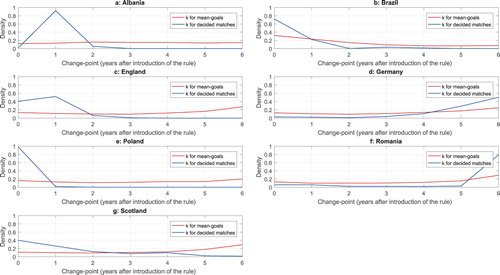
Finally, Figure A5 in the Appendix presents posterior distributions of the change-points, k, for the seven leagues, separately. One can easily see that while the curves corresponding to means goals are flat (indicating the data do not update the discrete uniform prior) the curves corresponding to proportions of decided matches have peaks at various points within the study period - thereby supporting the change-point model.

5. Comparison with the Shiryaev–Roberts change point detection scheme

An alternative approach common in the change-point literature is the Shiryaev–Roberts (SR) change point detection scheme [19,20] which, according to Vexler and Hutson [24], can also be considered as Bayes factor type test. Following the notation of our Section 3.2, the null hypothesis (no change) is $H_0:d_t\sim f_0=\mathrm{B}\mathrm{i}\mathrm{n}\left(N_t,\theta \right),t=1,\dots ,T$ while the alternative hypothesis (change) is $H_1:d_t\sim f_0=\mathrm{B}\mathrm{i}\mathrm{n}\left(N_t,\theta \right),t=1,\dots ,k{d}_t\sim f_1=\mathrm{B}\mathrm{i}\mathrm{n}\left(N_t,\lambda \right),t=k+1,\dots ,T.$ The Shiryaev–Roberts (SR) test statistic is then given by (see Chapter 4 in [24]): (20) $SR=\sum _{t=1}^{T}f\left(t\right)\frac{\int \prod _{t=k}^T{f}_1\left(d_t|\lambda \right)p\left(\lambda \right)\mathrm{d}\lambda }{\int \prod _{t=k}^T{f}_0\left(d_t|\theta \right)p\left(\theta \right)\mathrm{d}\theta },$(20) where $f\left(t\right)$ is the prior distribution of the change-point. Substituting the discrete uniform prior distribution assumed in Equation (13(13) $f\left(k\right)=\frac{1}{T}.$(13) ) the above test-statistic reduces to: (21) $S{R}_k^T=\frac{1}{T}\sum _{t=1}^T\frac{\int \prod _{t=k}^T{f}_1\left(d_t|\lambda \right)p\left(\lambda \right)\mathrm{d}\lambda }{\int \prod _{t=k}^T{f}_0\left(d_t|\theta \right)p\left(\theta \right)\mathrm{d}\theta }.$(21) The null hypothesis is rejected for large values of $S{R}_k^T$, say if $S{R}_k^T>$ C, where the critical value C can be found by Monte Carlo evaluations as described in Chapter 16 in Vexler et al. [25]. Chap. 12 of the same book [25] provides an example on computing the $S{R}_k^T$-statistic and comparing its power with that of the cumulative sum (CUSUM) method.

Application of the above test to our data on mean-goals and proportions of decided matches gave the results in Table 9.

Table 9. Results (in log-scales) from Shiryaev–Roberts change point detection tests.

		Albania	Brazil	England	Germany	Poland	Romania	Scotland
Mean Goals	SR-Stat.	5.70	10.25	3.78	5.48	2.69	0.90	1.88
	Crit. Value	7.13	7.12	7.15	7.08	6.98	7.22	7.12
Prop. decided	SR-Stat.	14.30	8.45	8.70	3.65	10.83	1.56	2.80
matches	Crit. Value	3.03	3.03	3.08	3.06	3.04	3.10	3.04

The results in the upper and lower panels of Table 9 are in accordance with those in Tables 6 and 8, respectively, except for the mean goals for Brazil and proportion of decided matches for Germany. In Tables 6 and  8 the Bayes factors for these entries showed insignificant evidence to reject the null hypothesis (of no change) while in Table 9 the null hypothesis is rejected. This difference can be explained by the fact that the Shiryaev-Roberts approach rejects the null hypothesis if the $S{R}_k^T$-statistic is larger than the critical value $\mathbf{C}$ (regardless of the size of the difference) while the Bayes factor provides information about the degree of evidence in support of the alternative hypothesis.

6. Discussion

We have proposed and applied a Bayesian change-point model to measure the effects of the 3-points-for-a-win rule in the football world. Our model is statistically well-grounded and, more importantly, much less subjective compared to previous approaches used to analyse the same data sets. One of the strengths in our approach is that we let the time for change, if any, to be part of the model and estimate it together with other parameters of interest.

Our results do not support a change-point model for mean goals in any of the leagues studied. On the other hand, the results provide strong evidence for a change-point model for the proportion of decided matches in most of the leagues studied. Such results were supported when we compared our method with the Shiryaev-Roberts method that is common in the change point detection literature.

This, in turn, implies that the 3pfaw rule has given teams the incentive to win matches (rather than draw). However, this was achieved not by scoring ‘too many’ goals but, rather, by scoring enough goals in order to win and, at the same time, defending enough in order not to lose.

For instance, a hypothetical match that could have ended in a 2-2 draw before the 3pfaw rule might end in a 1-0 or 2-1 win after the 3pfaw rule. Such a match contributes towards increasing the proportion of decided matches but not towards increasing the mean goals scored per match.

The current study is limited to only seven leagues and over a shorter period before and after the introduction of the 3pfaw rule (only about 7 years). This, in turn, corresponds to the 1990s (late 1970s to early 1980s in the case of England). However, our results are supported by the findings in Anderson and Sally's [1] book which is based mostly on league matches during the 2001/02–2010/11 seasons. One of the key findings reported in the book is that it was statistically more valuable to prevent a goal than to score one.

Nevertheless, future investigations can examine if our results hold over longer periods or for other leagues. They can also consider the literature on the uncertainty of outcome hypothesis as well as the new literature on surprise, suspense, upset, etc. and other factors influencing the change in goals scored over time.

Our hope is that the current contribution serves as an inspiration to investigators to attempt one or more of the extensions outlined above.

Acknowledgments

We are grateful to the Associate Editor who suggested us to compare our method to the Shiryaev–Roberts change point detection scheme and directed us to valuable references describing and illustrating the method [24,25]. This has given us a new insight for the present and future works. Comments from two anonymous referees were of great value in revising the paper. Previous versions of this paper [9] have been presented at two of the regular seminars at the Department of Statistics, Stockholm University and at the 27th Nordic Conference in Mathematical Statistics, Tartu (Estonia), 25–29 June 2018. The authors would like to thank participants at those occasions and particularly to Daniel Thorburn and Frank Miller of Stockholm University for constructive comments and suggestions.

Disclosure statement

No potential conflict of interest was reported by the authors.

ORCID

Gebrenegus Ghilagaber https://orcid.org/0000-0002-2910-8432

Correction Statement

This article has been republished with minor changes. These changes do not impact the academic content of the article.

Appendix

Figure A1. Trends in mean goals before and after introduction of 3pfaw rule across seven leagues.

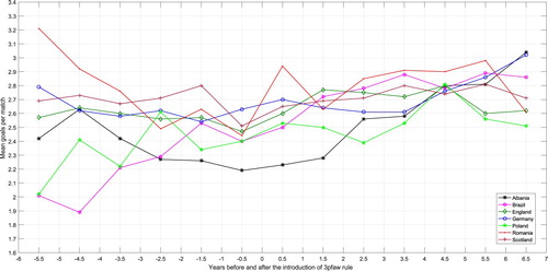
Figure A2. Trends in proportions of decided matches before and after introduction of the 3pfaw rule across seven leagues.

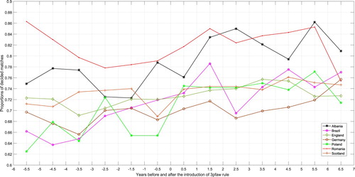
Figure A3. Posterior distributions of mean goals before and after the 3pfaw rule in seven leagues (a–g), change-points (h), and differences in mean goals (i).

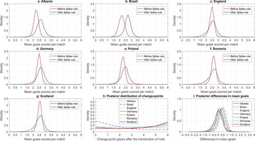
Figure A4. Posterior distributions of proportions of decided matches before and after the 3pfaw rule (a–g), change-points (h), and differences in proportions (i).

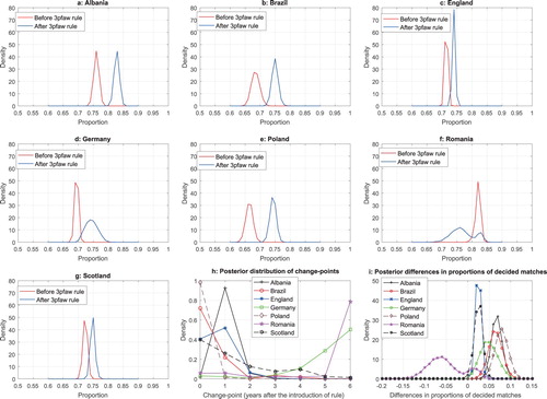
Figure A5. Posterior distributions of change-points (k) for mean-goals (red) and proportions of decided matches (blue) across the seven leagues studied.

References

- C. Anderson and D. Sally, The Numbers Game: Why Everything You Know About Footbal is Wrong, Penguin Books Ltd., London, 2014.
- M. Aylott and N. Aylott, A meeting of social science and football: Measuring the effects of three points for a win, Sport Soc. 10 (2007), pp. 205–222. doi: 10.1080/17430430601147047
- L. Bauwens and J.V.K. Rombouts, On marginal likelihood computation in change-point models, Comput. Statist. Data Anal. 56 (2012), pp. 3415–3429. doi: 10.1016/j.csda.2010.06.025
- I. Brocas and J.D. Carrillo, Do the “three-point victory” and “golden goal” rules make soccer more exciting?, J. Sports Econ. 5 (2004), pp. 169–185. doi: 10.1177/1527002503257207
- B.P. Carlin, A.E. Gelfand, and A.F.M. Smith, Hierarchical Bayesian analysis of change-point problems, Appl. Stat. 41 (1992), pp. 389–405. doi: 10.2307/2347570
- J.H. Chin Choy and L.D Broemeling, Some Bayesian inferences for a changing linear model, Technometrics 22 (1980), pp. 71–78. doi: 10.2307/1268385
- A. Dilger and H. Geyer, Are three points for a win really better than two? a comparison of German soccer league and cup games, J. Sports Econ. 10 (2009), pp. 305–318. doi: 10.1177/1527002508327521
- A. Dominicus, S. Ripatti, N.L. Pedersen, and J. Palmgren, A random change-point model for assessing variability in repeated measures of cognitive function, Stat. Med. 27 (2008), pp. 5786–5798. doi: 10.1002/sim.3380
- G. Ghilagaber and P. Munezero, Bayesian change-point modelling of the effects of 3-points-for-a-win rule in football, Research Report 2018:3, Department of Statistics, Stockholm University, 2018.
- J. Gill, Bayesian methods - a social and behavioral sciences approach, 2nd ed., Chapman and Hall/CRC, London, 2008.
- C.B. Hall, J. Ying, L. Kuo, and R.B. Lipton, Bayesian and profile likelihood change-point methods for modeling cognitive function over time, Comput. Statist. Data Anal. 42 (2003), pp. 91–109. doi: 10.1016/S0167-9473(02)00148-2
- L.Y. Hon and R.A. Parinduri, Does the three-point rule make soccer more exciting? evidence from a regression discontinuity design, J. Sports Econ. 17 (2016), pp. 377–395. doi: 10.1177/1527002514531790
- R.E. Kass and A.E. Raftery, Bayes factors, J. Am. Statist. Assoc. 90 (1995), pp. 773–795. doi: 10.1080/01621459.1995.10476572
- C.-B. Lee, Bayesian analysis of a change-point in exponential families with applications, Comput. Statist. Data Anal. 27 (1998), pp. 195–208. doi: 10.1016/S0167-9473(98)00009-7
- G.C. Moschini, Incentives and outcomes in a strategic setting: The 3-points-for-a-win system in soccer, Econ. Inq. 48 (2010), pp. 65–79. doi: 10.1111/j.1465-7295.2008.00177.x
- S. Petrone and A.E. Raftery, A note on the Dirichlet process prior in Bayesian nonparametric inference with partial exchangeability, Statist. Probab. Lett. 36 (1997), pp. 69–83. doi: 10.1016/S0167-7152(97)00050-3
- A.E. Raftery, Hypothesis testing and model selection, W.R. Gilks, S. Richardson and D. Spiegelhalter, eds., Markov Chain Monte Carlo in Practice, Chapman & Hall, New York, 1996, pp. 163–188.
- A.E. Raftery and V.E. Akman, Bayesian analysis of a Poisson process with a change-point, Biometrika 73 (1986), pp. 85–89. doi: 10.1093/biomet/73.1.85
- S.W. Roberts, A comparison of some control chart procedures, Technometrics 8 (1966), pp. 411–430. doi: 10.1080/00401706.1966.10490374
- A.N. Shiryaev, On optimum methods in quickest detection problems, Theory Probab. Appl. VIII (1963), pp. 22–46. doi: 10.1137/1108002
- G.K. Skinner and G.H. Freeman, Soccer matches as experiments: How often does the ‘best’ team win?, J. Appl. Stat. 36 (2009), pp. 1087–1095. doi: 10.1080/02664760802715922
- A.F.M. Smith, A Bayesian approach to inference about a change-point in a sequence of random variables, Biometrika 62 (1975), pp. 407–416. doi: 10.1093/biomet/62.2.407
- A. Van Den Hout, G. Muniz-Terrera, and F.E. Matthews, Change-point models for cognitive tests using semi-parametric maximum likelihood, Comput. Statist. Data Anal. 57 (2013), pp. 684–698. doi: 10.1016/j.csda.2012.07.024
- A. Vexler and A.D. Hutson, Statistics in the Health Sciences: Theory, Applications, and Computing, Chapman & Hall/CRC, Boca Raton, FL, 2018.
- A. Vexler, A.D. Hutson, and X. Chen, Statistical Testing Strategies in the Health Sciences, Chapman & Hall/CRC, Boca Raton, FL, 2016.
- B. Western and M. Kleykamp, A Bayesian change-point model for historical time series analysis, Polit. Anal. 12 (2004), pp. 354–374. doi: 10.1093/pan/mph023