Evaluation of robust outlier detection methods for zero-inflated complex data

ABSTRACT

Outlier detection can be seen as a pre-processing step for locating data points in a data sample, which do not conform to the majority of observations. Various techniques and methods for outlier detection can be found in the literature dealing with different types of data. However, many data sets are inflated by true zeros and, in addition, some components/variables might be of compositional nature. Important examples of such data sets are the Structural Earnings Survey, the Structural Business Statistics, the European Statistics on Income and Living Conditions, tax data or – as in this contribution – household expenditure data which are used, for example, to estimate the Purchase Power Parity of a country.

In this work, robust univariate and multivariate outlier detection methods are compared by a complex simulation study that considers various challenges included in data sets, namely structural (true) zeros, missing values, and compositional variables. These circumstances make it difficult or impossible to flag true outliers and influential observations by well-known outlier detection methods.

Our aim is to assess the performance of outlier detection methods in terms of their effectiveness to identify outliers when applied to challenging data sets such as the household expenditures data surveyed all over the world. Moreover, different methods are evaluated through a close-to-reality simulation study. Differences in performance of univariate and multivariate robust techniques for outlier detection and their shortcomings are reported. We found that robust multivariate methods outperform robust univariate methods. The best performing methods in finding the outliers and in providing a low false discovery rate were found to be the generalized S estimators (GSE), the BACON-EEM algorithm and a compositional method (CoDa-Cov). In addition, these methods performed also best when the outliers are imputed based on the corresponding outlier detection method and indicators are estimated from the data sets.

KEYWORDS:

• Outlier detection
• zeros
• robust methods
• household expenditures

2010 MATHEMATICS SUBJECT CLASSIFICATION:

• 62H86

1. Introduction

Data quality is an important issue in quantitative data analysis. A critical aspect of the data quality monitoring is outlier detection, especially also in data sets including missing values or/and zero-inflated variables. Classical statistical methods are sensitive to outliers and may be led, consequently, to a distorted picture of the reality due to the presence of outlier values, leading to erroneous conclusions. Therefore, the identification of values which either are obviously erroneous or may have high influence on statistical methods is a major task. Especially for large data sets the automatized detection of outliers becomes an important task.

A general view on outliers, historical remarks and literature:

In the literature the term outlier is not defined uniformly nor are the definitions for an outlier connected to only one mathematical formula. Many authors became aware of outliers already quite a long time ago. For example, [5] considered outliers in a rather philosophical manner in his Novum Organum. The choice of means in presence of outliers was investigated in [21]. Errors in measurements were already discussed in [37], and they introduced trimming as a sound statistical method [see also 33]. It was suggested to leave one (the largest observed value) out of five observed values. In the work [30] it was mentioned that ‘An outlier is an observation that deviates so much from other observations as to arose suspicion that it was generated by different mechanism’. And [6] wrote ‘An outlying observation, or outlier, is one that appears to deviate markedly from other members of the sample in which it occurs’. According to our study, we define an outlier as a data point that behaves differently than the majority of data points which are assumed to follow some underlying model; a similar definition can be found in [26].

Some of these attempts to define outliers are ‘rule based’ approaches – the identification by data specific edit rules developed by subject matter experts followed by deletion and imputation. However, these rules – even though efficient and important in many situations – are strictly deterministic and ignore the probabilistic component. In addition, they are extremely labour intensive. It should be noted that deterministic methods are not topic of this paper, and for details we refer to [16]. We also mention that outlier detection methods for time series are not the topic of this paper; we refer to [27,38]. Many univariate and multivariate outlier detection methods can be named, but only few can deal with complex data sets. As an example, the rank-based method of [31] is suited to detect outliers in continuous data sets without missing values and zeros. Even [30] already wrote that ‘the problem of outliers is one of the oldest in statistics’, but – as just mentioned – still there is a lack for outlier detection methods that account for problems with missing values, zero-inflation and special kinds of data such as compositional data and non-symmetric distributions. The paper [56] already considered outlier detection methods on complex business survey samples and compared also some methods that are evaluated in the following.

However, we want to go some steps further especially by discussing a greater variety of outlier detection methods and by allowing for more deviations from ‘normality’ in terms of missing values, zero-inflation and non-symmetric compositional distributions. These challenges are described in the following.

Missing values:

Especially survey data often contain missing values, therefore the outlier detection methods must be able to work with incomplete data, either by imputation of missing values in advance or by imputation procedures implemented within the method.

Zero-inflation:

In surveys on monetary values, often several monetary variables are collected in order to capture the economic situation of an entity [9]. This holds, for example, for business surveys, where many particular types of expenditures may be asked as this is the case for expenditure data collected by almost any state of the world and committed to the World Bank. Such kind of surveys are based on elaborated questionnaires; they typically include unit- and item non-responses and zero inflated distributions. Zero-inflation occurs because a particular entity usually only has information on a subset of the possible dimensions. The zero inflation occurs, for example, in multi-faceted economic situations. Not all people have, for example, income related to agriculture in income surveys, or not all retired persons may have labour income. For a non-smoking family it is also not very likely that they have expenditures on tobacco, for example. Only a few methods can deal with zero-inflated data. While for univariate methods the outlier detection method may just be applied to the observed part only, this is not a trivial problem in higher dimensions. Multivariate methods are often not designed to deal with this problem. Exceptions are, for example, the method of [9].

Non-symmetric distributions:

It is also challenging for outlier detection methods to deal with the size effect of families, farms or businesses and, very important, to deal with potential skewed distributions – in particular survey data are often skewed. Note that most of the univariate and multivariate outlier detection methods assume symmetric distributions, and an appropriate transformation of variables (or the use of special robust methods for skewed data [32]) is thus an important step before outlier detection algorithms are applied. Additional difficulties arise from compositional parts in a data set, where the components (e.g. household expenditure variables) are not independent from each other. For example, if the expenditures on alcohol and tobacco will be raised in a particular household, the household can (frequently) spend less money on other expenditures. This leads to compositional data analysis and to the log-ratio methodology [2,22] that has also been used recently for outlier detection [24,54].

Complex surveys and survey weights:

Survey data are mostly conducted with a complex sampling design leading to a possible different design weight for each individual. If so, the naming convention is to use the wording complex survey data. Through calibration procedures finally each individual is connected to a survey weight. Whenever one deals with complex surveys, mostly estimations are done in a weighted (design-based) manner. All univariate outlier detection methods investigated in this study consider sample weights, the epidemic algorithm [7] and the BACON-EEM method [8] is the only multivariate method considered in this study that can deal with survey weights.

True outliers, influential observations and outliers:

The previously given definitions about outliers do not distinguish between data points with extreme erroneous values (measurement errors, non-representative outliers), and data points which are true values but are too distant from the rest of the data so that they will have huge influence on classical estimators (representative outliers) [13]. In practice it has to be mentioned that it is not always possible to distinguish between measurement errors or a genuine, but very extreme observation. In general we thus use outlier methods to detect data points which have the potential of being an outlier. Such data points are sometimes also referred to as potential outliers.

Properties of robust methods:

Statistical outlier detection methods are usually built around some sort of robust statistical estimate. Such estimators are characterized by not being strongly influenced by outliers which enables them to produce reliable estimates although extreme values are present in the data. The robustness of an estimator T is typically characterized by either the 'influence function' (IF) or the 'breakdown point' (BP). The IF describes the sensitivity of a single outlier (or very small amount of contamination) on an estimator T, and for estimation methods, including various outlier detection methods, one prefers estimators T with bounded IF. Contrary to the IF, which describes the influence on the estimator T by small amounts of contamination, the breakdown point specifies the minimal amount of contamination for which the estimator is no longer able to produce a useful estimation value. The maximal achievable breakdown point is 50$\mathrm{\%}$, since for a value higher than 50$\mathrm{\%}$ the bigger share of the outliers could be considered 'genuine' data. Logically, an outlier detection method should itself not be influenced by outliers, thus any outlier detection method should be robust, optimally with a bounded IF, with a high breakdown point and high statistical efficiency.

Variety of methods:

Next to mostly non-robust outlier detection methods [see, e.g. 1] and hundreds of (mostly univariate) outlier detection methods, a broad variety of robust outlier detection methods exists in the literature. Such robust statistical methods have been studied for quite some time now and a variety of different methods has been developed not only for the purpose of detecting outliers, but also for gaining reliable estimations on data that are potentially corrupted by outliers or contain a lot of noise. Since the variety of robust statistical methods is quite large it can be difficult to assess which method is most appropriate for the underlying data sets. For a recent overview of outlier detection methods, see [60].

Outline of the paper:

In this work, we explore the impact of a variety of robust statistical outlier detection methods on large household expenditure data and finally assess their performance within a simulation study. The rest of this work is structured as follows: Section 2 will give a brief overview of the robust estimates which were used. Section 3 presents empirical results of these statistical outlier detection methods applied on one of the data sets, followed by Section 4 which presents a simulation study to assess the performance of the used outlier detection methods applied on large household expenditure data.

2. Methods under consideration

In the following, a pre-selected set of robust univariate and robust multivariate outlier detection methods is reviewed and evaluated.

Univariate methods – favored for their simplicity – can be informal graphical methods like histograms, boxplots, dot plots; quartile methods to create allowable ranges for the data, or robust methods, e.g. based on robust univariate location and scale estimates.

Multivariate methods are still rarely used in this context, although most of the surveys collect multivariate data.

2.1. Univariate methods

In terms of one-dimensional data, outliers are solely those points which are 'far enough' away from the main bulk of the data. In order to locate these points, one way is to estimate location and scale of a data sample in a robust way. For example, all observations which fall outside the range of location plus/minus a multiple of the scale can be considered as outliers. We did not consider non-robust methods because it is well-known that these methods cannot adequately detect outliers, and we did not consider methods based on quantiles, because hereby a number of observations are classified as outliers even if there are no outliers in a data set. The chosen methods are listed in Table 1 and briefly explained in the following.

Table 1. Overview of univariate and multivariate outlier detection methods addressed.

Kind	Method	Reference	Specifics
univariate	IQR	–	used in combination with Box-Cox transformation
	MAD	–	used in combination with Box-Cox transformation
	boxplot	–	very common outlier detection method
	adjusted boxplot	[58]	extension of boxplot for skewed data
	Pareto tail modelling	[4,20,35,59]	used for skewed data and uses sophisticated replacement of outlier
multivariate	M-estimate	[43]	generalization of Maximum Likelihood estimate
	S-estimate	[15,40]	high BP with low efficiency
	MM-estimate	[52]	high BP with high efficiency
	MCD-estimate	[47]	affine equivariant
	MVE-estimate	[47]	affine equivariant
	Stahel Donoho estimate	[18,50,51]	incorporates weights corresponding to the 'outlyingness' of a data point
	OGK-estimate	[17,44]	combines bivariate covariance estimator defined by [29] with PCA
	BACON-EEM	[8]	able to deal with missing values
	EA	[7]	simulates an epidemic in the data
	GSE	[14]	extension to S-estimate
	TSGS	[39]	treats cell-wise outliers before applying GSE
	CoDa-Cov	[54]	treats data in compositional context

As a robust estimator of location we use the Median, and for the scale either the interquartile range (IQR) or the median absolute deviation (MAD), both standardized to produce a normal-consistent estimate of the standard deviation. The constant was chosen equal to 3, since this represents a common outlier detection rule, and in case of normal distribution, the interval mean plus/minus 3 times standard deviation theoretically contains more than 99$\mathrm{\%}$ of the possible realizations.

Applying these methods to household expenditure data could yield problematic results since expenditure data are typically skewed to the right. Naturally, if it can be assumed that the distribution of a variable is log-normal, it would be reasonable to apply the logarithm, since this would lead to a symmetric normal distribution. However, this assumption does not always hold and we therefore used the Box-Cox transformation [11] to account for the skewness. The Box-Cox transformation relies on one parameter λ. For $\lambda =0$ it equals to the log-transformation. The appropriate value of λ can be estimated via maximum likelihood or a robust regression approach. The robust regression approach was taken into account since the Box-Cox transformation could be influenced by extreme values. Considering the sorted data values $0<x_1\le \dots \le x_i\le \dots \le x_n$, then the Box-Cox transformed values with the Box-Cox parameter λ are defined as $x_i^{(\lambda )}=(x_i^{\lambda }-1)/\lambda$ if $\lambda \ne 0$ and $x_i^{(\lambda )}=\log x_i$ otherwise. We consider the linear model (1) $x_i^{(\lambda )}=\alpha +\beta z_i+u_i,$(1) with α, β and λ as real parameters, and $z_i$ as the $i/n$th quantile of the standard normal distribution. Furthermore, the errors $u_i$ are considered i.i.d., independent of $z_i$ and $\mathbb{E}[u_i]=0$. Then the Box-Cox parameter λ can be estimated by applying MM-regression to the responses $x_i^{(\lambda )}$ for given λ, and λ is chosen such that the robust residual auto-correlation ${\rho }_n(\lambda )$ is minimized [42]. To combine the Box-Cox transformation with outlier detection we first transformed the data and applied the outlier detection methods, robust locations plus/minus constant times robust scale, on the transformed data. Afterwards the boundaries beyond which outliers can be found are transformed back and are applied onto the untransformed data to detect outliers.

Another univariate outlier detection method which can cope with right skewed data incorporates Pareto tail modelling [20,35]. By estimating a cut-off point beyond which a Pareto distribution can be fitted to the right tail of the data one can declare outliers as those points that are larger than a certain quantile of the fitted Pareto distribution. The cut-off point used was the Van Kerm's rule of thumb [57], and the Pareto distribution was fitted using a partial density component estimator [4,59].

In addition to the previously mentioned methods, the boxplot and the adjusted boxplot [58] were used to detect outliers in the univariate case. The adjusted boxplot adjusts the term $1.5\pm IQR$ of the original boxplot rule to better accomodate skewed data. Hereby, the medcouple (MC) [12] is used as a measure of skewness, and observations outside $[Q_1-1.5e^{-4MC}IQR;Q_3+1.5e^{3MC}IQR]$ are marked as outlier, with $Q_1$ and $Q_3$ being the first and third quantiles.

The data used contain survey sample weights. The sampling weights are considered for univariate outlier detection methods. For example, the median is replaced by the weighted median, the cut-off point and scale parameter of the semi-parametric Pareto tail modelling method are estimated in a weighted manner [4], etc.

2.2. Multivariate methods

For multivariate data the task of declaring outliers is not as simple as in the univariate case. Data points that are just ‘far’ away from the data centre do not need to be actual outliers. Instead, outliers in the multivariate case are data points that are not in correspondence with the structure of the main bulk of the data. A very prominent measure which incorporates the structure of the data is the so-called squared Mahalanobis distance $M{D}_i^2$. Given a data matrix $\mathbf{X}\in {\mathbb{R}}^{n\times p}$ with n observations ${\mathbf{x}}_i$, for $i=1,\dots ,n$, containing p measurements, the squared Mahalanobis distance for the i-th observation $M{D}_i^2$ is defined by (2) $M{D}_i^2=({\mathbf{x}}_i-\overline{\mathbf{x}}{)}^t{\mathbf{S}}^{-1}({\mathbf{x}}_i-\overline{\mathbf{x}}),$(2)

with $\overline{\mathbf{x}}$ as the sample mean and $\mathbf{S}$ as the sample covariance matrix. In case of data following a multivariate normal distribution the squared Mahalanobis distance $M{D}_i^2$ is approximately ${\chi }_p^2$ distributed with p degrees of freedom. Therefore, observations with high squared Mahalanobis distance are possible candidates for outliers. A common rule is to declare data points as outliers if they exceed the 97.5$\mathrm{\%}$ quantile of the ${\chi }_p^2$ distribution, ${\chi }_{p;0.975}^2$. The squared Mahalanobis distance, however, can be subject to so called masking and swamping [see also 48]. To address this problem it is necessary to use robust estimates for location and covariance. In the literature one can find many different robust estimators for location $\mathbf{T}$ and covariance $\mathbf{C}$ which differ in their statistical properties and in their computational efficiency.

The different robust estimators used are as follows (see also Table 1). The M-estimate [43] which presents a generalization of the Maximum Likelihood estimate. For the M-estimate it can be shown that the asymptotic breakdown point is bounded by $1/p$. For the empirical calculations a so called constrained M-estimate, also abbreviated with CM-estimate, as described in [46] was used.

The S-estimate [15,40] incorporates M-scale estimates with a robust estimation of the scale.

The MM-estimate [52] uses an S-estimate with high breakdown point as a preliminary scale estimate and combines this preliminary estimate with a 'better' tuned ρ-function to gain an efficient estimate with high breakdown point.

The minimum covariance determinant (MCD) and minimum volume ellipsoid (MVE) [47] estimate determines location and covariance by the covariance matrix of at least half of the data points, having a minimal determinant or minimal volume, respectively.

The Stahel Donoho [18,50,51] estimate incorporates weights corresponding to the 'outlyingness' of a data point. The OGK-estimate [17,44] uses the robust bivariate covariance estimator $s_{jk}$ proposed by [29] and combines it with a principal component decomposition.

The BACON-EEM [8] algorithm is composed of the BACON algorithm [10] starting from a robust centre and subsequently selecting observations. It has been modified by the authors to deal with sample weights and missing cells, e.g. when one or multiple values of an observation ${\mathbf{x}}_i$ are missing. The epidemic algorithm (EA) [7] starts an epidemic from the estimated centre of the data and is thus a density-based method. Similar to the BACON-EEM, the EA is able to deal with missing cells in the data. For the calculations the BACON-EEM was initialized using the squared marginal Mahalanobis distance and the EA was used in connection with the Euclidean distance and a linear transmission function. It has to be noted that the EA algorithm does not compute a robust estimate for location and covariance and this method was only used in addition to the other methods since it presents a very different approach to outlier detection.

The Generalized S-estimate (GSE) [14] and the Two-Step Generalized S-estimate (TSGS) [39] are extensions to the S-estimator that simultaneously deal with outliers and missing data. The TSGS even incorporates a preprocessing step to detect cell-wise outliers and sets them to missing before applying the GSE.

Finally, an outlier detection method which is a slight adaptation from the function compareMahal in the R-package robCompositions [53,54] is selected. This method can deal with missing cells and zeros, and treats the data as compositional data. A short description of this method applied to a data matrix $\mathbf{X}\in {\mathbb{R}}^{n\times p}$ works as follows:

1. Impute the missings and zeros in $\mathbf{X}$ with the k-nearest-neighbour algorithm [36], with k = 5, resulting in ${\mathbf{X}}_{imp}$.

2. Split ${\mathbf{X}}_{imp}$ into subsets according to the structure of the missing values or zeros in $\mathbf{X}$, meaning that every resulting subset contains only those observations which contained missing values or zeros in the same cells in $\mathbf{X}$.

3. For each subset rearrange the order of the columns in ${\mathbf{X}}_{imp}$ such that all columns that did contain missing values or zeros in $\mathbf{X}$ for this subset are listed first.

4. Apply the isometric log-ratio transformation [22] to ${\mathbf{X}}_{imp}$ with reordered columns and calculate the covariance estimate using the Minimum Covariance Estimator [49].

5. In each subset use the parts of the covariance matrix, where the subset had no missing values or zeros in $\mathbf{X}$. Calculate robust Mahalanobis distances and use a threshold rule (based on ${\chi }^2$ distribution), see [54].

It has to be noted that this method only detects outliers regarding the composition of an observation (in fact, the ratios between the variables are taken) and it does not consider the absolute values. Note that the method itself relies on (a specific) isometric log-ratio transformation. Since this isometric log-ratio transformation is permutation invariant, it can be shown that the outlier detection method is also permutation invariant, i.e. reordering of the variables in a data set does not change the results. This method will be denoted as CoDa-Cov for the rest of this paper. Note that with this approach outliers can be detected on subsets even if they contain more columns than rows.

For reasons of clarity, the presented outlier detection methods are – as already mentioned – summarized in Table 1.

2.3. Replacement of outliers

Obviously, the aim of this study is to detect outliers and not to impute them. However, in the numerical studies we also aim to estimate indicators from the data sets where outliers are automatically detected by an outlier detection method and then modified specifically to the outlier detection method. This allows to not only consider false discovery rates in simulation studies, but also to evaluate the estimation of important indicators, which is the main issue for the used data sets for organizations like the World Bank.

Univariate outliers are replaced by either the upper or lower boundary which declare the range of ‘good’ data points. As for the Pareto tail modelling, outliers are replaced by resampling values from the fitted distribution [see also 3].

Multivariate outliers are replaced by winsorizing them onto the 97.5$\mathrm{\%}$ tolerance ellipse, created by the robust estimate of location and covariance. In the case of the EA and the BACON-EEM the algorithms do not produce robust estimates of location and covariance. To achieve comparable results between the methods, the 97.5$\mathrm{\%}$ tolerance ellipse is created by classical estimates of location and covariance from all infected data points, in case of the EA and in case of the BACON-EEM the estimates of location and covariance from the last steps are used to create the tolerance ellipse. For the CoDa-Cov method the tolerance ellipses are calculated for each subset using the needed parts of the corresponding MCD estimate.

3. Empirical results

3.1. Provided data and data structure

The data used were provided by the World Bank and contain household expenditure data from five different countries, namely Albania, Mexico, India, Malawi and Tajikistan. The household data sets resulted from large household surveys conducted in each of these countries in the years 2007, 2008, 2010, 2009, and 2010 respectively. In order to use the same methodology and terminology the data sets were harmonized by the World Bank [19] using a standardized framework for goods and services, namely the basic headings used by the International Comparison Program (ICP) 2005. Besides socio-demographic characteristics of each household as well as information on the household structure, including household size, education and age structure of the household members, the data sets include yearly household expenditures in local currency. The yearly household expenditures of each data set are factorized by 4 different category codes, namely the ICP basic headings, the ICP class, the ICP group and ICP category, for which every code represents a rougher grouping of the former. For the ICP basic headings, consisting of 107 different expenditure categories, the number of zeros in each category is quite substantial throughout all data sets. Therefore, we used the roughest grouping (ICP category), containing 13 main expenditure categories. Even when analysing only the main categories, the amount of zeros can for some categories exceed 50$\mathrm{\%}$ of the corresponding sample size. In some cases the amount is even over 80$\mathrm{\%}$ or 90$\mathrm{\%}$ of the sample size.

A common non-robust estimator that is calculated with household expenditure data is the so called Gini coefficient [28,41]. In this context the Gini coefficient measures the inequality of expenditures in terms of monetary value between the surveyed households. Since the data were generated through large surveys, extreme values or measurement errors can occur, with a potential effect on the Gini coefficient [see also 4]. Therefore, it would be beneficial to detect and impute outliers beforehand. An important issue was that the position of true outliers was not known beforehand and neither was the true value of the Gini coefficient. Nevertheless, looking at the value of the Gini coefficient after different outlier detection methods and adjustments have been applied, gives insight on how strongly these detection schemes influence the level of the Gini coefficient.

3.2. Data preparation

Before applying the outlier detection methods one must first deal with the zeros in the data. In case of univariate outlier detection methods, if a household should happen to have no listed yearly expenditures it will be discarded for the outlier detection. For the multivariate case the high number of zeros would heavily influence the robust estimates for location and covariance. Therefore, these zeros will be treated as missing values and imputed before outlier detection. The algorithms which are able to deal with missing values are the EA, the BACON-EEM, the GSE, the TSGS and the CoDa-Cov. For the other methods it is necessary to select a pre-processing step. In order to keep the influence of the missing values to a minimum they will be imputed using the k-nearest-neighbour algorithm [36], with k = 5.

3.3. Numerical results

Results have been derived from the data from all five countries, however, the results from one country (Albania) are in focus here in order to stay in the page limits. This data set consists of 3600 observations on households, and it was already investigated in a technical report by the authors, see [23]. We extend these analyses in the following.

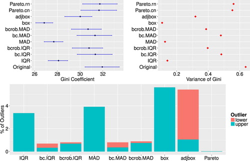
For the underlying data the univariate outlier detection methods were applied on the total household expenditures per household. The results shown in Figure 1 present on the top left side the estimated values for the Gini coefficient after the outlier detection schemes have been applied and outliers have been adjusted. IQR, MAD, box and adjbox indicate the use of the interquartile range, the median absolute deviation, the boxplot or the adjusted boxplot for outlier detection. The abbreviations bc and bcrob indicate that in these cases the Box-Cox transformation and the robustification of the Box-Cox transformation, respectively, were applied together with the IQR or MAD. For Pareto modelling the detected outliers have either been replaced by values drawn from the fitted Pareto distribution (denoted by Pareto.rn), or the corresponding weights for the outliers have been set to 1 and the weights for the other observations have been re-calibrated accordingly (denoted by Pareto.cn) [4,23]. The 95$\mathrm{\%}$ confidence intervals for the estimated Gini coefficients are represented by blue horizontal lines. The variances of the estimated Gini coefficient can be found for all univariate outlier detection methods in Figure 1, top right. The variances and confidence intervals of the Gini coefficient were calculated with a bootstrap (100 bootstrap replicates), in which the sample weights are re-calibrated in every bootstrap sample using geographical information provided by the data sets. The percentages of detected outliers are shown on the bottom barchart (Figure 1). The different colours indicate upper and lower outliers. It can be seen that only outlier detection methods which do account for skewed data detect lower outliers. Furthermore, the number of flagged outliers by those detection schemes that do not account for skewness is rather substantial. In combination with the top part of Figure 1 it is clear that the corresponding Gini coefficients are heavily influenced after the adjustment of these outliers. Except for the Pareto tail modelling approach, methods which adjust for the skewness of the data detect quite a large number of lower outliers. For the adjusted boxplot method, the number of lower outliers is especially high and thus this method performs not well in this case. The detection of lower outliers might be important in general, but the influence of lower outliers on the Gini coefficient is small. In other words, if the data contain true outliers and the estimated Gini coefficient thus will be biased, then this is mainly caused by upper outliers.

Figure 1. Top: Estimates of the Gini coefficient (left) and variance of the Gini coefficient (right) for the Albanian data set after univariate outlier detection methods as well as outlier imputation have been applied. Bottom: Share of upper and lower outliers for each outlier detection scheme applied to the Albanian data set.

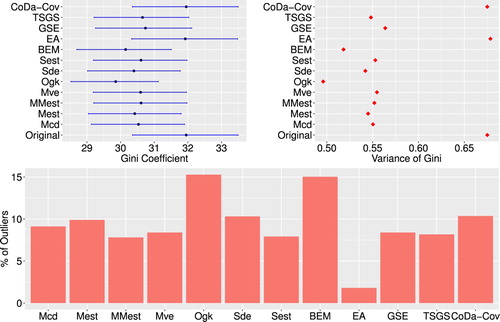
The multivariate outlier detection methods are applied on the household expenditure data set using the ICP category code. To summarize, the used estimators or methods consist of the M-estimator (Mest), the MM-estimator (MMest), the S-estimator (Sest), the MCD estimator (Mcd), the MVE estimator (Mve), the Stahel-Donoho estimator (Sde), the OGK estimator (Ogk), the epidemic algorithm (EA) the BACON-EEM (BEM), GSE (GSE), the TSGS (TSGS) and the CoDa-Cov method (CoDa-Cov). The R-package modi is used to calculate the BACON-EEM and the epidemic algorithm, for the calculation of the GSE and TSGS the R-package GSE is used, and for the CoDa-Cov method the code is available in the R-package robComposition. The rest of the robust estimates for location and covariance were calculated with the R-package rrcov [55]. Many of these methods have tuning parameters affecting e.g. the breakdown point or the efficiency. We used the default parameters as they are implemented in the R-package rrcov. For most of the methods the household expenditure data were log-transformed beforehand. This was necessary since most of the methods rely on elliptical symmetry of the data distribution. For the EA and the CoDa-Cov method the data were not transformed by the logarithm. The former does not require the data to be of elliptical shape and the latter treats the data in a compositional context.

Figure 2 shows the results for the estimates for the Gini coefficient and share of detected outliers for each multivariate outlier detection method applied to the Albanian household expenditure data. In contrast to the case of univariate outlier detection methods, the results for the Gini coefficients do not differ so much among the applied methods. Only the results for the OGK estimator, the epidemic algorithm and the CoDa-Cov differ slightly more from the results of the other methods. The same can be noted for the share of detected outliers. The results for the multivariate outlier detection methods are quite similar and it is therefore not clear which of the multivariate methods performed best. Even in comparison with the use of univariate methods it is not clear if univariate or multivariate outlier detection methods should be preferred. To address this problem, we conducted a simulation study to see how the different methods performed on data which were generated based on the Albanian household expenditure data.

Figure 2. Top: Estimates of Gini coefficient (left) and variance of Gini coefficient (right) for the Albanian data set after multivariate outlier detection methods as well as outlier imputation have been applied. Bottom: Share of outliers detected by multivariate outlier detection methods for the Albanian household data.

4. Simulation study

This simulation study extends results already partly presented in a technical report of the authors, see [23]. Due to the fact that the number and position of the ‘real’ outliers in the data sets are unknown and there is no knowledge about a ‘true’ Gini value, it is difficult to decide which method performs ‘better’ in the sense of ‘more reliable’. Differences in the performance are expected just by the different theoretical properties of the estimators. Furthermore, one could expect that multivariate methods outperform univariate methods just becasue multivariate information is used. However, this is not as clear when we are interested in estimating an indicator such as the Gini coefficient. A simulation study should give deeper insights.

The simulation study addresses two important issues:

1. Simulate a data set that represents important properties of the data set provided by the World Bank.

2. The number and position of ‘true’ outliers must be known.

4.1. Simulated data

We generate data for which the distribution is based on the distribution of the expenditure data from the Albanian data set. It is important to note that expenditure data listed by expenditure categories are considered as compositional data, therefore we will take this into account when generating new data. Our design to simulate data consists of the following steps:

1. The zeros in the Albanian data set are first imputed using the k-nearest-neighbour algorithm [36].

2. Since the data are considered as compositional data, the data set is first represented in orthonormal isometric logratio (ilr) coordinates. Since the specific choice of ilr coordinates would not alter the results, we represent the data in pivot coordinates, see [25].

3. The data set in ilr coordinates is split into a 'clean' and a 'contaminated' data set. The former one should contain most likely no outliers whereas the latter should contain mostly outliers. Univariate as well as multivariate outlier detection schemes applied previously were used to partition the observations into the two groups. More precisely, the clean data set contains only observations that have not been flagged by any of the outlier detection schemes as outliers. This resulting data set consists of 2687, out of 3600, most likely uncontaminated observations. The contaminated data set contains observations that were flagged as outliers by the majority of the outlier detection methods. These are all observations that were flagged as outliers by at least 6 univariate outlier detection methods or at least 8 multivariate outlier detection methods. The contaminated data set consists of 311 observations.

4. From the contaminated and clean data set the location and covariance are estimated in a classical way and used as a basis for the distribution of the simulated data set.

5. This resulting simulated data set follows a classical contamination scheme. More precisely, let $({\mathit{\mu }}_{cl},{\mathbf{\Sigma }}_{cl})$ and $({\mathit{\mu }}_{co},{\mathbf{\Sigma }}_{co})$ be classical estimates of location and covariance of the clean and contaminated data set, respectively, then the simulated data set $\mathbf{X}$ follows the following distribution (3) $\mathbf{X}\sim (1-ϵ)MVN({\mathit{\mu }}_{cl},{\mathbf{\Sigma }}_{cl})+ϵMVN({\mathit{\mu }}_{co},{\mathbf{\Sigma }}_{co}),$(3) with $ϵ\in (0,1)$ determining the share of contaminated data points. As the Albanian data set, the simulated data set is also constructed with 3600 observations.

6. For the contamination (for further discussions on outlier mechanisms, see [34]), observations were picked at random and

   1. replaced by the data simulated from a multivariate normal distribution with $({\mathit{\mu }}_{co},{\mathbf{\Sigma }}_{co})$.

   2. for a share of all the randomly picked observations to be contaminated, not the whole observation but just one randomly chosen cell is contaminated. Given the $i^{th}$ observation for which only the $j^{th}$ cell will be contaminated, the cell is replaced by $y_{ij}$, with $\mathbf{Y}\sim MVN({\mathit{\mu }}_{co},{\mathbf{\Sigma }}_{co})$. This addition to the contamination scheme was also implemented since such structures can be expected for real expenditure data sets and there is no real reason why such kind of contamination should not occur.

7. To obtain data that are more comparable with the original Albanian data set, the data are transformed back to the simplex by using the inverse ilr transformation. The resulting columns are multiplied by the columnwise centred means of the original data set in order to obtain the original scale of the Albanian data set.

8. The number of zero-observations can be quite high and play quite a big role for the analysis of such data sets. The simulated data will therefore contain zeros. To ensure a realistic distribution of the zero-observations we copied the structure of the zero-observations from the whole Albanian data set and applied this to the simulated data. This means that we assigned zeros to each cell in the simulated data where zeros have been found in the Albanian data set. The percentages of values beeing zero varies between the variables and ranges from less than 0.2% to 41%. By replacing values in the simulated data set with zeros, it can occur that previously generated artificial outliers will be replaced by those zeros. Since the data are simulated many times and the placement of zeros overlapping with the randomly chosen contaminations is not very likely, it is expected that there is not a large impact on the simulation study.

9. Sample weights also play quite a role for the presented outlier detection methods as well as for the Gini calculation. Thus, the simulated data sets receive the same sample weights as the household weights given in the Albanian data set.

4.2. Application of univariate methods

In order to be able to estimate indicators like the Gini coefficient, an outlier detection method is applied on each column of the data set, and the detected outliers are imputed for each column seperately. The main reason for this approach is that in this way the results are more comparable between the univariate and multivariate outlier detection methods. In addition, univariate outlier detection methods will make use of the household sample weights. Note that for the univariate outlier detection methods the zeros are discarded for calculating and imputing outliers.

4.3. Application of multivariate methods

For multivariate outlier detection methods, zeros are treated as missing values (as in correspondence with [56] and [54]). For some outlier detection methods, the resulting missings are imputed prior to outlier detection by using the k-nearest-neighbour algorithm ([36]). Imputation of missing values is only for the purpose of outlier detection, and afterwards the imputed values are again replaced by zeros. In the case of the epidemic algorithm, BEM, TSGS, GSE and CoDa-Cov, the missing values do not need to be imputed.

In the univariate as well as in the multivariate case, the number of correctly identified artificial outliers and falsely declared outliers are counted. Furthermore, applying the outlier detection methods and imputing outliers generates new data sets which correspond the each of the used outlier detection methods. For these data sets, the weighted Gini coefficient for the sum of the expenditures per observation is calculated.

In the simulation procedure different levels of ε, $ϵ\in \{0,0.01,0.025,0.05\}$ were taken. In total, 50 simulation runs for each setting are taken, and the average number of correctly identified artificial outliers and falsely declared outliers are reported. As discussed for the outlier simulation, for a part of the contaminated data only one cell of each observation is contaminated, and for the rest of the contaminated data, the whole observation is contaminated. For the simulation, 1/3 of the contamination is cell-wise and for 2/3 of the contaminated data the whole observation is contaminated. At first the results for the univariate outlier detection methods are discussed.

4.4. Simulation results

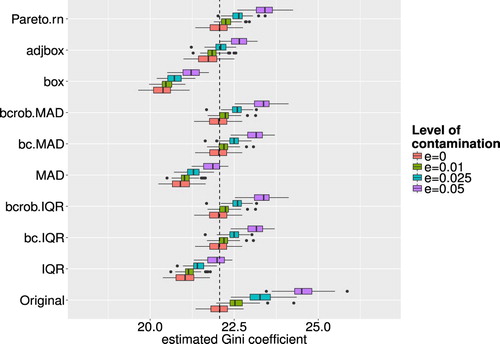
The estimated Gini coefficients for each univariate method and each level of ε are shown in Figure 3. From Figure 3 it is interesting to see that for higher values of ε the values for the Gini coefficient increase, even when outlier detection and imputation have been applied beforehand. This seems strange since the outlier detection schemes are supposed to identify and impute the outliers in order to reduce the effect of the outliers on an estimate. However, for the outlier imputation, except in the case of the Pareto modelling, the outliers are winsorised onto the interval boundaries, whereas these boundaries are calculated during the detection methods, imputed outliers still have an influence on the Gini. Nevertheless, this trend is rather small and for outlier detection schemes which take into account skewness of the data, the resulting Gini is still quite close to the one with no contamination and no outlier detection scheme applied.

Figure 3. Estimated Gini coefficients for different levels of ε and different outlier detection methods. The dashed line indicates a baseline representing the median of the Gini coefficients of the uncontaminated data.

It is also crucial to see successfully detected outliers (whole observation contaminated), which is shown in Figure 4 for different levels of ε and the investigated outlier detection methods. The legend indicates the ratio of artificial outliers. The methods were not successful in detecting outliers. For higher values of ε, the performance on outlier detection got worse. Moreover, using the Box-Cox transformation was not as successful at identifying outliers for this scenario. Looking at the szenario where only one single cell was contaminated, the outlier detection methods performed not well either. These results are visualized in Figure 5 (compare also [23]). In opposite to the row-wise contaminations, the results for the cell-wise contamination does not show as drastic differences between the univariate methods. Pareto modelling performed poor in this setting, but the reason for this is given by the fact that Van Kerm's rule of thumb is used, which suggests after which threshold the Pareto distribution is fitted. This suggestion might not be suitable for this simulation with outliers shifted with other means. The Pareto method is suited for fitting heavy-tailed distributions, but does not cope well with distributions that have separated support, such as the pointwise-outliers which are far away from the main bulk of the data in our simulation setup. The results for the Pareto modelling are therefore not satisfactory. Regarding the successful detection of outliers it can be said that the boxplot, adjusted boxplot and the methods using IQR or MAD without Box-Cox transformation were able to identify comparatively more artificial outliers than the other detection methods. However, to get a clearer picture of the performance of the methods it is important to consider the number of falsely flagged outliers as well.

Figure 4. Boxplots of successfully detected artificial outliers, where the whole observation was contaminated, for different outlier detection methods and different levels of ε.

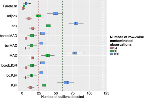
Figure 5. Boxplots of successfully detected artificial outliers, where only single cells were contaminated, for different outlier detection methods and different levels of ε.

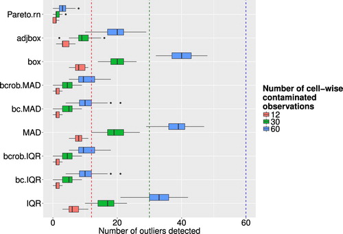
Figure 6 shows the corresponding boxplots for different outlier detection methods and different levels of ε. The x-axis corresponds to the share of flagged outliers to the total amount of clean data in the simulated data set. Except for methods like the Pareto modelling or methods which incorporate the use of the Box-Cox transformation the number of falsely flagged outliers is especially high. One could even argue that the numbers for methods which use the Box-Cox transformation are too high. The high amount of falsely flagged outliers in the case of the boxplot, adjusted boxplot and the methods using IQR or MAD without Box-Cox transformation put in perspective their relatively better performance regarding the ability to correctly identify artificial outlier. Therefore, one can argue that these methods are not precise for outlier detection in this kind of data. From the results shown above, the use of univariate outlier detection schemes, or at least the column-wise use of those methods does not seem appropriate for this kind of data. The ability to detect artificial outliers was not very satisfactory and the number of falsely flagged outliers was far too high in almost all cases. This can also be seen in Table 2, which shows the average misclassification rate for each univariate method and different levels of ε.

Figure 6. Share of false/positive outliers to number of clean data points for different outlier detection methods and different levels of ε.

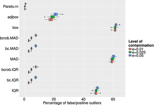
Table 2. Percentages of misclassified observations for different levels of ε for the univariate methods.

Method	ε = 0.01	ε = 0.025	ε = 0.05
Pareto.rn	1.21	2.82	5.43
adjbox	18.35	20.17	23.39
box	60.99	60.68	60.59
bcrob.MAD	3.84	6.69	11.37
bc.MAD	3.84	6.77	11.31
MAD	59.00	58.89	59.12
bcrob.IQR	3.84	6.69	11.35
bc.IQR	3.84	6.75	11.28
IQR	48.37	48.42	49.17

Similar to the univariate outlier detection methods, Figure 7 shows the boxplots of the Gini values for the different multivariate outlier detection methods and different levels of ε. The Gini estimates for the epidemic algorithm as well as the CoDa-Cov method are still heavily influenced by the artificial outliers. For the epidemic algorithm this can be explained by the fact that this algorithm needs quite a lot of tuning for parameter calibration until it is really applicable to a problem. Since we used the default parameter settings in our simulation study we cannot argue that the algorithm is bad but it is not very versatile without meaningful calibration which differs depending on the underlying data. The CoDa-Cov method treats the data in a compositional context and therefore does not detect or impute outliers on row totals, for which the Gini coefficient is estimated. For the other outlier detection methods one can see, as in the case of univariate outliers, an increase in the Gini coefficient for rising levels of contamination. As it was argued for the univariate case, this is caused by the imputation, which does not perfectly replace an outlier by winsorising it onto the 97.5$\mathrm{\%}$ tolerance ellipse. Thus a rising number of outliers leads to a rising number of observations lying on the boundary of the 97.5$\mathrm{\%}$ tolerance ellipse. The data points of the resulting data set are therefore wider spread from the centre of the data than the data points in the uncontaminated data set. This difference in the distribution of the data can finally be seen in values of the Gini coefficients for different levels of ε. Apart from that the results for the multivariate outlier detection methods do – especially for higher levels of ε – not differ too much from the case where the data were not contaminated.

Figure 7. Boxplots of calculated Gini coefficients for different outlier detection methods and different levels of ε. The dashed line indicates a baseline representing the median of the Gini coefficients of the uncontaminated data.

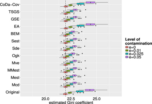
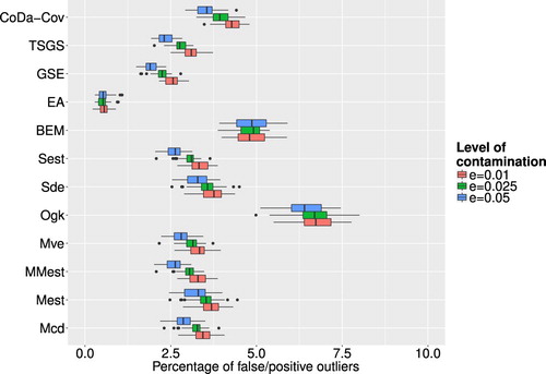
Figure 8 corresponds to artificial outliers for which the whole observation was contaminated and Figure 9 corresponds to those where only one cell was contaminated. Regarding the row-wise outliers, the multivariate outlier detection methods were much more successful than the univariate methods, not considering the epidemic algorithm. In many cases, the algorithms were able to detect every artificial outlier and even for increasing values of ε the numbers are still very high. The epidemic algorithm did not perform too well, but as stated earlier this is due to poor calibration of parameters, which is in practice a very cumbersome task. The results in Figure 9 show that none of the methods was particularly successful in detecting cell-wise artificial outliers. This can on one hand be explained by the fact that none of the chosen multivariate outlier detection methods is especially suited for detecting outlying cells in contrast to outlying observations. On the other hand, the artificially created outlying cells where generated in the real space, and detecting them in the transformed compositional space can be especially challenging. For the case of falsely flagged outliers regarding multivariate outlier detection methods, Figure 10 shows the resulting boxplots for different outlier detection methods and different levels of contamination. Compared to the univariate case the number of falsely flagged outliers is far smaller for the multivariate outlier detection schemes. The OGK estimator seems to perform not so well as it has a higher number of falsely flagged outliers than the other methods. For $ϵ=0.01$ the majority of the multivariate outlier detection schemes have roughly the same amount of falsely flagged outlier and the share increases slightly with rising values of ε. Looking at all multivariate outlier detection methods, except the epidemic algorithm that was ruled out as valid method beforehand, the GSE delivers the least amount of falsely flagged outliers.

Figure 8. Boxplots of successfully detected artificial outliers, where the whole observation was contaminated, for different outlier detection methods and different levels of ε.

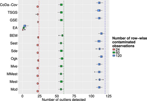
Figure 9. Boxplots of successfully detected artificial outliers, where only single cells were contaminated, for different outlier detection methods and different levels of ε.

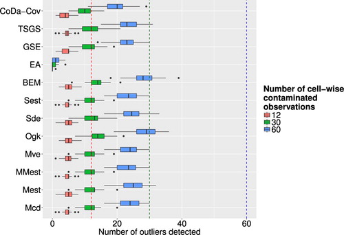
Figure 10. Boxplots of share of false/positive outliers to number of clean data points for different outlier detection methods and different levels of ε.

The average misclassification rates, shown in Table 3, increase for most of the methods only slighty with increasing ε, which also supports the notion that multivariate outlier detection methods did quite well in most of the cases.

Table 3. Percentages of misclassified observations for different levels of ε regarding multivariate methods.

Method	ε = 0.01	ε = 0.025	ε = 0.05
CoDa-Cov	4.50	4.50	4.72
TSGS	3.32	3.31	3.50
GSE	2.78	2.79	3.10
EA	1.51	2.93	5.38
BEM	5.04	5.21	5.65
Sest	3.54	3.59	3.75
Sde	3.92	4.05	4.32
Ogk	6.90	7.00	7.16
Mve	3.50	3.63	3.91
MMest	3.50	3.55	3.73
Mest	3.87	3.99	4.29
Mcd	3.64	3.75	3.98

To conclude it can be said that the multivariate outlier detection methods all performed very well, also compared to univariate outlier detection methods. That only leads to the conclusion that univariate outlier detection methods are less suited for the detection of outliers in large household expenditure data whereas multivariate outlier detection methods can deal better with the complexity of this problem and deliver therefore more satisfactory results.

5. Conclusions

Data sets often include difficulties for outlier detection algorithms that have not been investigated in detail, like dealing with missing and zero values, skewness and compositional nature of the data as well as possible complex sampling designs of surveys. The outlined methods for univariate and multivariate outlier detection can be considered as the (large) set of possible methods available in the statistics literature. The methods differ in their need for preprocessing (e.g. imputation of missing values), distributional assumptions, but also in the sensitivity and specificity to identify outliers.

One general conclusion from the simulation but also from the application to real-world data is that univariate outlier detection methods must be adapted for skewness. Depending on the applied outlier detection method, a univariate outlier in original scale must not be an outlier in, e.g. log-scale. Without a transformation to achieve a more symmetric distribution or methods that account for skewness internally (adjusted boxplot, Pareto method), univariate outlier detection methods might simply declare larger data values (e.g. in right-skewed data) as outliers. Thus, these methods should be used with care in practice if data are skewed. Especially for the expenditure data (but also from the simulation results) we see that the adjusted boxplot method detected too many outliers in the left tails of the distributions. The Pareto method seems to detect too few outliers. Methods based on the robust (and non-robust) Box-Cox transformation combined with a robust estimation of variance gave the most reasonable results for the univariate methods.

For the expenditure data set, no clear picture about differences between the methods for multivariate outlier detection can be detected. Only EA and OGK behave clearly different, which is an indication that they underestimate (EA) and overestimate (OGK) the number of outliers.

The simulation study, which was conducted based on the information of one of the data sets, gave additional insights. We used the number of correctly identified artificial outliers and falsely declared outliers for the evaluation of the methods. The results from the simulation study highlighted that multivariate outlier detection methods are more suitable for outlier detection for household expenditures, because (i) they detected a very high share of artificial and true outliers and (ii) they flagged only few false/positive outliers. Overall, multivariate outlier detection methods were more precise than univariate rules in terms of correctly identifying outliers and in terms of smaller amounts of incorrectly flagged outliers. Out of the tested methods only the Epidemic Algorithm (EA) delivered poor results, which was mainly based on using the default values of the tuning parameters. Other methods are less dependent on tuning constants and the determination of its optimal values. The results might be improved by chosing better tuning constants. However, for real-world data sets this is complicated, because the number of outliers is unknown. The OGK estimator gave slightly worse results in terms of the percentage of false/positive outliers, but all other methods behave similarly. The BEM method performed best for the correct number of true outliers identified, but a higher percentage of false/positive outliers was detected. The GSE method provided good results for a combination of both, the numbers of true outliers detected and the percentage of false/positive outliers. Interesting is the fact that the method CoDa-Cov leads to approximately the same results as other multivariate outlier detection methods. From the theoretical properties, this method should be most suitable, but the simulation results do not confirm this.

For outlier detection in data collected with a complex survey design, survey weights should be considered. Further research is thus needed to adapt the methods for complex survey designs. The BACON-EEM (BEM) and the Epidemic Algorithm (EA) can deal with weights, but other multivariate methods do not consider the sampling weights.

Finally, we want to emphasize that after the application of outlier detection methods, a careful analysis of the detected outliers is necessary for any of the methods.

The calculations have been done using the programming language R [45], version 3.5.3.

Disclosure statement

No potential conflict of interest was reported by the authors.

ORCID

M. Templ http://orcid.org/0000-0002-8638-5276

Correction Statement

This article has been republished with minor changes. These changes do not impact the academic content of the article.

References

- C. Aggarwal, Outlier Analysis, Springer, New York, 2013.
- J. Aitchison, The Statistical Analysis of Compositional Data, Chapman & Hall, London, 1986.
- A. Alfons and M. Templ, Estimation of social exclusion indicators from complex surveys: the R package laeken, J. Stat. Softw. 54 (2013), pp. 1–25. doi: 10.18637/jss.v054.i15
- A. Alfons, M. Templ and P. Filzmoser, Robust estimation of economic indicators from survey samples based on Pareto tail modelling, J. R. Stat. Soc. C-Appl. 62 (2013), pp. 271–286. doi: 10.1111/j.1467-9876.2012.01063.x
- F. Bacon and J. Devey, Novum Organum, in Library of universal literature: Science, P. F. Collier (ed.), 1902.
- V. Barnett and T. Lewis, Outliers in Statistical Data, Wiley Series in Probability & Statistics, Wiley, 1994.
- C. Béguin and B. Hulliger, Multivariate outlier detection in incomplete survey data: the epidemic algorithm and transformed rank correlations, J. R. Stat. Soc. Ser. A 167 (2004), pp. 275–294. doi: 10.1046/j.1467-985X.2003.00753.x
- C. Béguin and B. Hulliger, The BACON-EEM algorithm for multivariate outlier detection in incomplete survey data, Surv. Methodol. 34 (2008), pp. 91–103.
- M. Bill and B. Hulliger, Incomplete business survey data, Aust. J. Stat. 45 (2016), pp. 3–23. doi: 10.17713/ajs.v45i1.86
- N. Billor, A.S. Hadi and P.F. Vellemann, BACON: blocked adaptative computationally-efficient outlier nominators, Comput. Stat. Data Anan. 34 (2000), pp. 279–298. doi: 10.1016/S0167-9473(99)00101-2
- G.E.P. Box and D.R. Cox, An analysis of transformations, J. R. Stat. Soc. B Meth. 26 (1964), pp. 211–252.
- G. Brys, M. Hubert and A. Struyf, A robust measure of skewness, J. Comput. Graph. Stat. 13 (2014), pp. 996–1017. doi: 10.1198/106186004X12632
- R. Chambers, A. Hentges and X. Zhao, Robust automatic methods for outlier and error detection, J. R. Stat. Soc. A Stat. 167 (2004), pp. 323–339. doi: 10.1111/j.1467-985X.2004.00748.x
- M. Danilov, V.J. Yohai and R.H. Zamar, Robust estimation of multivariate location and scatter in the presence of missing data, J. Am. Stat. Assoc. 107 (2012), pp. 1178–1186. doi: 10.1080/01621459.2012.699792
- P.L. Davies, Asymptotic behavior of S-estimators of multivariate location parameters and dispersion matrices, Ann. Stat. 15 (1987), pp. 1269–1292. doi: 10.1214/aos/1176350505
- T. De Waal, Statistical data editing, in: Handbook of Statistics 29A. Sample Surveys: Design, Methods and Applications, D. Peffermann and C. Rao, eds., Elsevier B. V., Amsterdam, The Netherlands, 2009, pp. 187–214.
- S.J. Devlin, R. Gnanadesikan and J.R. Kettenring, Robust estimation of dispersion matrices and principal components, J. Am. Stat. Assoc. 76 (1981), pp. 354–362. doi: 10.1080/01621459.1981.10477654
- D.L. Donoho, Breakdown properties of multivariate location estimators, Ph.D thesis, Harvard University, Boston 1982.
- O. Dupriez, Building a household consumption database for the calculation of poverty PPPs, Technical Note, Draft 1.0, World Bank 2007.
- D. Dupuis and M.P. Victoria-Feser, A robust prediction error criterion for Pareto modelling of upper tails, Can. J. Stat. 34 (2006), pp. 639–658. doi: 10.1002/cjs.5550340406
- F. Edgeworth, Xxxiii. the choice of means, Philos. Magaz. Ser. 5 24 (1887), pp. 268–271. doi: 10.1080/14786448708628093
- J. Egozcue, V. Pawlowsky-Glahn, G. Mateu-Figueras and C. Barceló-Vidal, Isometric logratio transformations for compositional data analysis, Math. Geol. 35 (2003), pp. 279–300. doi: 10.1023/A:1023818214614
- P. Filzmoser, J. Gussenbauer and M. Templ, Detecting outliers in household consumption survey data, Tech. rep., Vienna University of Technology, Vienna, Austria, deliverable 4. Final Report. Contract with the world bank (1157976), 2016.
- P. Filzmoser and K. Hron, Outlier detection for compositional data using robust methods, Math. Geosci. 40 (2008), pp. 233–248. doi: 10.1007/s11004-007-9141-5
- P. Filzmoser, K. Hron and M. Templ, Applied Compositional Data Analysis, Springer Series in Statistics, Springer, Cham, 2018.
- P. Filzmoser, A. Ruiz-Gazen and C. Thomas-Agnan, Identification of local multivariate outliers, Statistical Papers 55 (2014), pp. 29–47. doi: 10.1007/s00362-013-0524-z
- R. Fried, Robust filtering of time series with trends, J. Nonparametr. Stat. 16 (2004), pp. 313–328. doi: 10.1080/10485250410001656444
- C. Gini, Variabilitae mutabilita, Tipografia di Paolo Cuppin, Tipogr. di P. Cuppini, Bologna, 1912, pp. 221–382.
- R. Gnanadesikan and J.R. Kettenring, Robust estimates, residuals, and outlier detection with multiresponse data, Biometrics 28 (1972), pp. 81–124. doi: 10.2307/2528963
- D. Hawkins, Identification of Outliers, Monographs on applied probability and statistics, Chapman and Hall, London, New York, 1980.
- H. Huang, K. Mehrotra and C. Mohan, Rank-based outlier detection, J. Stat. Comput. Simul. 83 (2013), pp. 518–531. doi: 10.1080/00949655.2011.621124
- M. Hubert and E. Vandervieren, An adjusted boxplot for skewed distributions, Comput. Stat. Data. Anal. 52 (2008), pp. 5186–5201. doi: 10.1016/j.csda.2007.11.008
- B. Hulliger, Johann Heinrich Lambert: an admirable applied statistician, Bullet. Swiss Stat. Soc. 14 (2013), pp. 4–10.
- B. Hulliger, A. Alfons, P. Filzmoser, A. Meraner, T. Schoch and M. Templ, Robust methodology for laeken indicators, Research Project Report WP4 – D4.2, FP7-SSH-2007-217322 AMELI, 2011.
- C. Kleiber and S. Kotz, Statistical Size Distributions in Economics and Actuarial Sciences, John Wiley and Sons, Hoboken, NJ, 2003. ISBN 0-471-15064-9.
- A. Kowarik and M. Templ, Imputation with the R package VIM, J. Stat. Softw. 74 (2016), pp. 1–16. doi: 10.18637/jss.v074.i07
- J.H. Lambert. Lambert's Photometrie. Translation into German by E. Anding. Wilhelm Engelmann, Leibzig, 1760/1892. Original work in Latin published 1760 by Klett.
- H. Lee and Y. Van Hui, Outliers detection in time series, J. Stat. Comput. Simul. 45 (1993), pp. 77–95. doi: 10.1080/00949659308811473
- A. Leung, V. Yohai and R. Zamar, Multivariate location and scatter matrix estimation under cellwise and casewise contamination, 2016. Available at arXiv:1609.00402
- H.P. Lopuhaä, On the relation between S-estimators and M-estimators of multivariate location and covariance, Ann. Stat. 17 (1989), pp. 1662–1683. doi: 10.1214/aos/1176347386
- M.O. Lorenz, Methods for measuring the concentration of wealth, Amer. Stat. Assoc. 9 (1905), pp. 209–219.
- A. Marazzi and V. Yohai, Robust Box-Cox transformations based on minimum residual autocorrelations, Comput. Stat. Data Anal. 50 (2006), pp. 2752–2768. doi: 10.1016/j.csda.2005.04.007
- R.A. Maronna, Robust M-estimators of multivariate location and scatter, Ann. Stat. 1 (1976), pp. 51–67. doi: 10.1214/aos/1176343347
- R.A. Maronna and R.H. Zamar, Robust estimation of location and dispersion for high-dimensional datasets, Technometrics 44 (2002), pp. 307–317. doi: 10.1198/004017002188618509
- R Core Team, R: A Language and Environment for Statistical Computing, R Foundation for Statistical Computing, Vienna, Austria, version 3.5.3. 2019.
- D.M. Rocke, Robustness properties of S-estimators of multivariate location and shape in high dimension, Ann. Stat. 24 (1996), pp. 1327–1345. doi: 10.1214/aos/1032526972
- P.J. Rousseeuw, Multivariate estimation with high breakdown point, in: W. Grossmann, G. Pflug, I. Vincze, and W. Wertz, eds., Mathematical Statistics and Applications Vol. B, Reidel Publishing, Dordrecht, 1985, pp. 283–297.
- P.J. Rousseeuw and A.M. Leroy, Robust Regression and Outlier Detection, John Wiley & Sons Inc., New York, NY, 1987.
- P.J. Rousseeuw and K. Van Driessen, A fast algorithm for the minimum covariance determinant estimator, Technometrics 41 (1999), pp. 212–223. doi: 10.1080/00401706.1999.10485670
- W.A. Stahel, Breakdown of covariance estimators, Research Report 31, ETH Zürich, Fachgruppe für Statistik 1981.
- W.A. Stahel, Robuste Schätzungen: Infinitesimale Optimalität und Schätzungen von Kovarianzmatrizen, Ph.D. thesis no. 6881, Swiss Federal Institute of Technology (ETH), Zürich 1981.
- K.S. Tatsuoka and D.E. Tyler, The uniqueness of S and M-functionals under nonelliptical distributions, Ann Stat 28 (2000), pp. 1219–1243. doi: 10.1214/aos/1015956714
- M. Templ, K. Hron and P. Filzmoser, robCompositions: An R-package for Robust Statistical Analysis of Compositional Data, John Wiley and Sons, Hoboken, NJ. 2011.
- M. Templ, K. Hron and P. Filzmoser, Exploratory tools for outlier detection in compositional data with structural zeros, J. Appl. Stat. 44 (2017), pp. 734–752. doi: 10.1080/02664763.2016.1182135
- T. Todorov and P. Filzmoser, An object oriented framework for robust multivariate analysis, J. Stat. Softw. 32 (2009), pp. 1–47. doi: 10.18637/jss.v032.i03
- V. Todorov, M. Templ and P. Filzmoser, Detection of multivariate outliers in business survey data with incomplete information, Adv. Data. Anal. Classif. 5 (2011), pp. 37–56. doi: 10.1007/s11634-010-0075-2
- P. Van Kerm Extreme incomes and the estimation of poverty and inequality indicators from EU-SILC, IRISS Working Paper Series, 2007-01, CEPS/INSTEAD 2007.
- E. Vandervieren and M. Hubert, An adjusted boxplot for skewed distributions, Comput. Stat. Data Anal. 52 (2008), pp. 5186–5201. doi: 10.1016/j.csda.2007.11.008
- B. Vandewalle, J. Beirlant, A. Christmann and M. Hubert, A robust estimator for the tail index of Pareto-type distributions, Comput. Stat. Data Anal. 51 (2007), pp. 6252–6268. doi: 10.1016/j.csda.2007.01.003
- A. Zimek and P. Filzmoser, There and back again: Outlier detection between statistical reasoning and data mining algorithms, WIREs Data Mining and Knowledge Discovery, 8, doi:10.1002/widm.1280