A comparison study on modeling of clustered and overdispersed count data for multiple comparisons

Abstract

Data collected in various scientific fields are count data. One way to analyze such data is to compare the individual levels of the factor treatment using multiple comparisons. However, the measured individuals are often clustered – e.g. according to litter or rearing. This must be considered when estimating the parameters by a repeated measurement model. In addition, ignoring the overdispersion to which count data is prone leads to an increase of the type one error rate. We carry out simulation studies using several different data settings and compare different multiple contrast tests with parameter estimates from generalized estimation equations and generalized linear mixed models in order to observe coverage and rejection probabilities. We generate overdispersed, clustered count data in small samples as can be observed in many biological settings. We have found that the generalized estimation equations outperform generalized linear mixed models if the variance-sandwich estimator is correctly specified. Furthermore, generalized linear mixed models show problems with the convergence rate under certain data settings, but there are model implementations with lower implications exists. Finally, we use an example of genetic data to demonstrate the application of the multiple contrast test and the problems of ignoring strong overdispersion.

Keywords:

• Generalized estimation equations
• overdispersion
• simultaneous contrast tests
• repeated measurements
• generalized linear mixed models

1. Introduction

The appearance of count data is very common in many different fields of science: applied ecology [31], pharmacology [29], toxicology [10], and genetic biology [25]. Frequently, the count data do not originate from independent samples, but from samples clustered according to biological habitats, litters, leaves from the same plant or the cells from the same petri dish. A model must consequently take both treatment effects and cluster effects into account. Furthermore, multiple comparisons within treatment types or genetic variants as well as the comparison of different habitats to a control group are often of scientific interest. Since Hothorn et al. [11] multiple contrast test are available for simultaneous confidence intervals. The user can define the contrasts for the scientific problem and use the parameter estimates from regression models to construct the confidence intervals.

Count data by nature does not follow a Gaussian, but a Possion distribution. Nonetheless, a simple, ordinary quadratic model, which requires a normal distribution, is often applied to analyze the count data. If the Poisson distribution is chosen appropriately, the limitation of its parameterization is very often neglected because the Possion distribution has only one shape parameter for the location of the mean. Therefore, the variance of the data is modeled as a linear function of the mean. Hence, if the variance increase exceeds the increase of the mean overdispersion θ occurs. In the case of a Poisson distribution we expect the variance to increase at a ratio of 1:1 to the mean. Therefore, we define the occurrence of overdispersion θ, if the mean/variance ratio exceeded two, i.e. $\theta >2$. From the practical point of view, a fitted model can be checked for overdispersion by dividing the residual deviance by the residual degrees of freedom. Beside these two problems of clustered data and overdispersion, the limitation effect of a small sample size can be observed while fitting the model parameters.

Sources for over-dispersion are many: variability of experimental material, correlation or dependence between individual sample responses, a clustered structure of the population, small sample size and even more [14,36]. As a special case overdispersion can be caused by high proportion of zeros as well as by zero truncation. Both these scenarios are very special cases and hence not considered in this paper.

The neglection of overdispersion is an underestimated standard error in the parameter estimates [22]. Therefore, the comparison of treatment effects will cause more significant results and therefore an increase of false positive findings. In contrast to non-significant results, significant results tend not to be questioned. As a result, the applied user will gain some sort of false benefit from neglection of overdispersion.

There are two solutions to deal with overdispersed count data. One, considering a distribution that is capable of estimating the mean and variance independently, e.g. the negative binomial distribution. Two, considering a quasi-distribution that allows to adjust the mean/variance ratio. In the case of the Poisson distribution, we can use the quasi-Poisson distribution. Ver Hoef and Boveng [33] stated, that the quasi-Poisson regression might be a better solution. This is driven by the fact that the negative binomial gives smaller sites more weight than the quasi-Poisson distribution. In our work the simulated settings we will run do not cover overdispersion caused by a high proportion of zeros and therefore expect estimates, which are not dominated by smaller counts.

There are two ways of modeling cluster effects: conditional or marginal models. Conditional models are more known by their common name linear mixed models (LMM), while marginal models are better known as generalized estimating equation (GEE). A well written review about the theoretical background can be found in Muff et al. [24]. In the case of the conditional model the correlation between the subjects in cluster is modeled. In contrast, the marginal model tries to consider the variance caused by each individual. Therefore the marginal models can interpreted as population average models. Lee and Nelder [17] stated, that the there are meaningless differences between conditional and marginal models due to the false interpretation of the effects. However, conditional models should have more advantages than marginal models. The statements of Lee are discussed controversially in the comments and rejoinder of Lee's article [17]. For a more comprehensive theoretical comparison of (G)LMM, as conditional models, and GEE, as marginal models, we want to refer to Zhang et al. [37]. In our work, we concentrate on the estimates of the mean differences and the goodness of variance estimators in the context of multiple contrast tests.

The applied statistician has the choice of different R packages for the multiple group comparisons of overdispersed count data with clustered samples: (generalized) linear mixed models, glmer(), using the R package lme4 [2], generalized estimating equations, geeglm(), using geepack [9] and in addition to the geeglm() the package geesmv [34]. The functionality of geesmv is needed for the selection of modified variance estimators adjusting for small sample size. The glmer() function in lme4 is not able to use the negative binomial distribution family. Therefore, the package introduce a additional function glmer.nb(). However, this function is called experimental and suboptimal, because of development processes. If the practical statistician would use the generalized mixed model functionality, he has to apply the Poisson distribution to the data. On the other hand, the standard lmer() functionality can be used on log transformed data, assuming normal distributed data after transformation. Newer implementations of the generalized linear mixed model exists: glmmADBM [32] and glmmTMB [20]. Both packages depend on the Template Model Builder (TMB) [16] and allow to use the negative binomial family for the analysis, while the glmmTMB offers more functionality [4]. In our work we concentrate on the implementations in R. However, there are different other statistical softwares and implementations of especially linear mixed models. Huang et al. [12] gives a comprehensive comparison of parameter estimations of linear mixed models in SAS and R. In case of SAS, the estimated coefficients of the linear mixed models can be extracted and added manually to the multcomp procedure in R.

Finally, the R package geepack allows users to use the generalized estimating equations for the estimation of the mean differences of the treatment groups. The usage of the Poisson family and the variance estimation on the individual level by the GEE model allow for the adjustment of possible overdispersed data. Nevertheless, generalized estimating equations present a broad variability of variance sandwich estimators. The choice of the right variance estimator has big influence of the final outcome of the estimation.

In our work we extend the work of Orelien et al. [27], which demonstrated the usage of generalized estimating equation model estimates for many-to-one comparisons. Since multiple contrast test are available [11] and different approaches for the analysis of clustered data have been introduced. Concretely, we extend the work of Orelien et al. [27] by using different contrast tests: Dunnett, Tukey, Williams, and Changepoint. In addition, we use generalized linear models for the multiple comparisons. Finally, we compare in a simulation study the different models estimate from linear mixed models and GEE for overdispersed clustered count data. We discuss different analysis settings and give advice for the practical use of the models under small sample size.

2. Methods

2.1. Data generation

We generated for the simulations study a data set consisting of one treatment effect $\text{β}$ and a additive cluster effect $\mathit{\gamma }$. The treatment vector $\text{β}$ consist always of four treatments $(nt=4)$. In the simulation different numbers of clusters per treatment $ct=\{2,3,4,5,10\}$ and samples per cluster $cs=\{2,3,4,5,10\}$ have been generated. Moreover, the count data set is build using different predefined overdispersions of $\theta =\{1,3,5,7,10\}$, and different effects of the cluster ${\acute{\lambda }}_{\gamma }=\{0.1,0.25,0.5,1,1.5\}\times {\lambda }_{\text{β}}$ in comparison to the treatment counts of ${\lambda }_{\text{β}}=\{10,10,10,10\}$. If one variable is not varied in the simulation, we set the number of clusters per treatment to three $(ct=3)$, the number of samples per cluster to four $(cs=4)$, the overdispersion to three $(\theta =3)$, and the cluster effect to ${\acute{\lambda }}_{\gamma }=0.5\times {\lambda }_{\text{β}}$.

The response variable Y is drawn from a negative binomial distribution. We were able to generate count data with overdispersion θ as the desired mean/variance ratio by using the ecological parameterization of the negative binomial distribution using the functionality of rnbinom() in R [3]. We set the scale parameter size to the desired mean/variance $\lambda /(\theta -1)$ and mu to the desired mean count λ. If the dispersion should be 1, we draw the counts from a Poisson distribution with the mean λ. We draw from a negative binomial distribution with a ${\lambda }_{\text{β}}=10$ for the fix treatment effect and with a ${\lambda }_{\gamma }=Pois(\lambda ={\acute{\lambda }}_{\gamma })$ for the random cluster effect. The resulting counts for the treatment effect $\text{β}$ and the cluster effect $\mathit{\gamma }$ are then added to the response variable Y. Supplementary Figure 1 shows a example data set with ${\lambda }_{\text{β}}=10$ and ${\lambda }_{\gamma }=Pois(\lambda =5)$. We checked if the predefined overdispersion θ matched the estimated overdispersion $\hat{\theta }$ using a generalized linear model fit with two fix effects including the treatment $\text{β}$ and a additive cluster effect $\mathit{\gamma }$ (Supplementary Figure 2). We determined $\hat{\theta }$ by dividing the residual deviance of the model fit by the residual degrees of freedom. We achieve a overall matching of the predefined and estimated overdispersion. We show in Supplementary material section 2 the R implementation of the data generation, if the reader might be more familiar with R code and find code in general easier to read.

2.2. Models for the simulation

The Table 1 shows the different models used in the simulation and example data analysis. Overall four models have been used in the simulation study: loglmm, a linear mixed model on log transformed count data assuming a normal distribution, glmm.pois, a generalized linear mixed model with a fixed effect and a random effect assuming a Possion distribution, glmm.tmb, a newer implementations of the generalized linear mixed models with a fixed and random effect modeling a negative binomial distribution, and GEE, generalized estimating equations with a fix effect and a random effect under a Possion distribution. All models are fitted using the mean parameterization and therefore removed the intercept from the model fit. In the following, we describe the used models for the simulation in more detail. The corresponding R implementations and code can be found in the Supplementary material section 2.

Table 1. Applied models in the simulation study and for the analysis of the example data set.

Model	R function (Package)	Fix effect	Cluster	Distribution
loglmm	lmer (lme4${}^{\ast }$)	$\text{β}$	$\mathit{\gamma }$	$\log (\mathbf{Y}+1)\sim Normal$
glmm.pois	glmer (lme4${}^{\ast }$)	$\text{β}$	$\mathit{\gamma }+\mathit{\delta }$	$\mathbf{Y}\sim Poisson$
glmmtmb.nb	glmmTMB (glmmTMB${}^{†}$)	$\text{β}$	$\mathit{\gamma }$	$\mathbf{Y}\sim NegBinom1$
GEE	geeglm (geepack${}^{\text{§}}$)	$\text{β}$	$\mathit{\gamma }$	$\mathbf{Y}\sim Poisson$
glm.pois	glm (stats)	$\text{β}+\mathit{\gamma }$		$\mathbf{Y}\sim Poisson$
glmm.nb	glmer.nb (lme4${}^{\ast }$)	$\text{β}$	$\mathit{\gamma }$	$\mathbf{Y}\sim NegBinom$

Notes: The upper four models have been used for the simulation. The lower two models were additionally added models for the analysis of the example data set: $\text{β}$ the fix effect of the treatments, $\mathit{\gamma }$ the random effect of the cluster, and $\mathit{\delta }$ the individual random effect in the glmm.pois model. The model glmm.nb has problems with the convergence rate and was therefore not used in the simulation study (Supplementary Figure 4). NegBinom1 has a variance function that increases linearly with the mean [7].

${}^{\ast }$Bates et al. [2].

${}^{†}$Magnusson et al. [20].

${}^{\text{§}}$Hojsgaard et al. [9].

The model loglmm solves the problem of overdispersed data by transforming the count data by a log-transformation. After the log-transformation the data can be seen as normal distributed. Therefore, a normal linear mixed model can be used to fit the model. Due to the log-transformation zero counts can not be modeled. Hence, all counts are increased by one, to remove zeros from the data set. The increasing is especially problematic in the case of a high proportion of zeros or small count numbers. In our simulation study, we consider mean counts of 15 and therefore we can apply the log-transformation. The final model includes a fix effect term $\text{β}$ for the treatment effects and a random effect term $\mathit{\gamma }$ for the cluster effects. We use the R package lme4 [2] and the function lmer() for fitting the model.

The second model glmm.pois models the data on the Poisson distribution. A negative binomial or quasi-Poisson family is not available for the glmer implementation in lme4. Hence, the modeling of the overdispersion is not possible by selecting the correct distribution. To solve this problem, we run the glmm.pois model with an additional random effect $\mathit{\delta }$ to model the individual effect. The additional parameter $\mathit{\delta }$ allows now to model the overdispersion by modeling the individual variance. The full glmm.pois model has a fix effect term $\text{β}$ for the treatment effects, a random effect for the cluster effects $\mathit{\gamma }$, and a additional random effect $\mathit{\delta }$ to model the individual effect of each sample. We use the R package lme4 [2] and the function glmer() to achieve the model estimates.

The third model glmm.tmb is a newer implementation of the generalized linear mixed models in R. The glmm.tmb allows to select a negative binomial distribution to model the overdispersion. Moreover, two negative binomial distributions are implemented: NegBinom1 has a variance function that increases linearly with the mean and NegBinom2 assumes a quadratic increase [7]. Therefore, we are able to use the glmm.tmb model with a fix effect term $\text{β}$ for the treatment effects and a random effect for the cluster effects $\mathit{\gamma }$. We use the R package glmmTMB [20] and the function glmerTMB() to fit the model.

Finally we used the GEE model. The model fit has been done twofold: first to estimate the fix effects for the the treatments using geepack and in a second step to estimate the variance covariance matrix of the fix effects using geesmv. For the usage of geesmv nine different sandwich variance estimators can be chosen and are available in R: [5,6,13,19,21,23,28,35]. We run a simulation study (Supplementary Figure 3) to determine the best sandwich variance estimator for our later simulation setting. The sandwich estimator proposed by Wang and Long [35] delivers far the best results. Nevertheless, Wang and Long (2011) pointing out, that their sandwich estimator works only on balanced data. Further, we use the function geeglm() from the R package using geepack [9] to fit the model for the treatment effects. In addition we choose a different sandwich estimator from the package geesmv [34] using the function GEE.var.wl() for the sandwich estimator by Wang and Long [35].

Two further models were used for the analysis of the example data set: glm.pois, a generalized linear model with two fix effects and ignoring the overdispersion, and glmm.nb, a generalized linear mixed model with a fix and random effect modeling a negative binomial distribution. The glm.pois model is used to demonstrate the misleading behavior of ignoring overdispersion in the analysis of the example data set. The glmm.nb model shows problems with the convergence rates of the fitting process. Therefore, the glmm.nb model does not converge and a warning is given. This was especially problematic with the varied overdispersion parameter (Supplementary Figure 4). Therefore we removed the model from the simulation.

After fitting the different model, we used for the multiple comparisons the estimated treatment effects $\stackrel{\mathbf{ˆ}}{\text{β}}$ from the mean parameterization and the extracted variance/covariance matrix with the standard errors from the model fits. Both can be included into the functionality of multcomp [11] and used for the multiple contrast test. While the generalized linear models of the lme4 package run without intervention in multcomp, the estimated parameters of the other models must be first extracted from the model fits and implemented by the user.

We run two simulation studies on different data settings. First, a simulation study to estimate the type I error or the coverage probability $(1-\alpha )$ with $\alpha =5\mathrm{\%}$ for all four contrast test. Second, a simulation study to achieve the power or rejection probability $(1-\text{β})$ with an twofold effect of treatment four. Hence the treatment effects for the power simulation study are ${\lambda }_{\text{β}}=\{10,10,10,20\}$. In our work, we define the power determined in a multiple comparison setting as global power [8]. Hence the probability of rejecting at least one null hypothesis independently if the corresponding comparison is truly under the alternative. By using this type of global power definition, we will have an enrichment of the power by comparisons, which are truly under the null, i.e. a power inflation by type I errors. We run for the type I error and power simulation 2500 replications.

3. Results

3.1. Simulation study on type I error

The simulation study of the coverage probability $(1-\alpha )$ reveals the GEE model as the best model in holding the family wise error rate among all settings (Figure 1). The GEE model has a coverage probability of nearly $95\mathrm{\%}$ independent of the cluster size, the cluster number per treatment, the cluster effect, or the dispersion parameter. Notable, the GEE models shows a small tendency to be more conservative. Overall, the GEE model can handle the clustered overdispersed data for all four contrast tests. Nevertheless, the performance is driven by the right choice of the variance sandwich estimator. If the variance estimator is false specified, because of unbalanced data or missing data points, the performance will be different. Hence, the usage of the right sandwich estimator is crucial (Supplementary Figure 3).

Figure 1. Coverage probability of the multiple comparisons using different contrast tests with four different models to fit the mean differences of the treatments and the standard errors of the means. If one variable is not varied in the simulation, the number of clusters per treatment is set to three $(ct=3)$, the number of samples per cluster to four $(cs=4)$, the overdispersion to three $(\theta =3)$, and the cluster effect to ${\acute{\lambda }}_{\gamma }=0.5\times {\lambda }_{\text{β}}=5$. There was no effect between the treatments. 2500 simulations have been run.

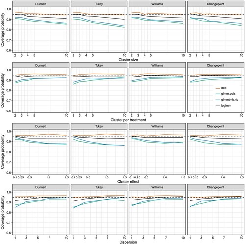
The second best model is the log-transformed linear mixed model. The loglmm model becomes to liberal in the case of a higher cluster size of 10 or with an increase of the cluster effect. In the case of low dispersion $(1<\theta <3)$ the log transformation lmm is also to liberal. There is no setting where the loglmm model becomes to conservative. In our simulation setting with moderate count numbers with a median of 15, the loglmm model can be used. As an advantage, the model runs very stable and converged in all settings. It is questionable, if the performance will be as good, if the number of counts decreases to a median near zero or the data has a high proportion of zeros.

The glmm and glmm.tmb models show nearly the same behavior, while the glmm.tmb model outperforms the glmm model slightly in the cases of cluster effect and dispersion. Nevertheless, the glmm.tmb model does not converge for no dispersion $(\theta =1)$ and is too liberal with a small cluster size of two. A cluster size of two is very small, but could be produced due to missing with larger initial cluster sizes. The glmm model runs with convergence warnings, but is able to estimate the model parameters. Overall the glmm model delivers the worst coverage probabilities. In combination with the convergence warnings of the glmm model the glmm.tmb models should finally be preferred over the glmm.

The convergence rate of the glmer() and the glmer.nb() function of the package lme4 was an overall observed problem. Especially, the application of the glmer.nb model using the negative binomial distribution is complicate (Supplementary Figure 4). If the overdispersion is high enough $\theta >10$, the model will converge in nearly 100% of the cases. On the other hand, if a low overdispersion can be observed, the model fit will not work properly in our simulation example. Therefore, we can not recommend the usage of the glmer.nb function, especially the experimental state is explicitly stated in the function description. In the case of the glmm model, the treatment effects and the standard errors of the parameters seemed not be biased. However, the glmmTMB package provides the functionality of generalized linear mixed models with a negative binomial distribution without convergence warnings.

3.2. Simulation study on power

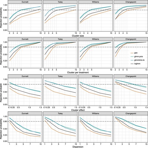
The simulation study of the rejection probability $(1-\text{β})$ shows that a reasonable number of clusters per treatment, larger than four, should be given to achieve a power of $80\mathrm{\%}$ (Figure 2). In addition, a larger cluster size also helps to reach the threshold of the rejection probability. Nevertheless, the number of clusters per treatment has a larger effect. Further, as expected with a increase of the cluster effects, the power decreases. The larger effects of the clusters cover the twofold effect of the treatment four. The same direction can be observed with an increase of the dispersion. While the glmm.pois and the glmmtmb.nb outperforms the GEE model, it must be remembered, that the power is inflated by the type I error rate, which is lower in the linear mixed models. Hence, the linear mixed models will find more significant results, but not necessarily under the true contrast. As a overall result, a small sample size will strongly decrease the rejection probability. Hence, it is better to use more clusters per sample, larger than four, with a moderate sample size per cluster, four to six.

Figure 2. Rejection probability of the multiple comparisons using different contrast tests with four different models to fit the mean differences of the treatments and the standard errors of the means. Treatment four has an twofold effect in comparison to the other treatments. If one variable is not varied in the simulation, the number of clusters per treatment is set to three $(ct=3)$, the number of samples per cluster to four $(cs=4)$, the overdispersion to three $(\theta =3)$, and the cluster effect to ${\acute{\lambda }}_{\gamma }=0.5\times {\lambda }_{\text{β}}=5$. There was no effect between the treatments. 2500 simulations have been run.

3.3. Example data set on genetic counts

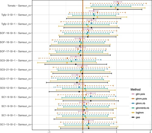
The following genetic data set was kindly provided by Prof. Dr Debener from the Institute for Plant Genetics at Leibniz Universität Hannover. We analyzed a count data set with 13 different tomato plant genotypes which can be considered as treatments as well as a negative control called ‘Samsun_cv’ and positive control called ‘Tomato’. Hence, we achieved a total number of 15 treatment groups (nt = 13 + 1 + 1 = 15). On each of the tomato plants three leafs were examined and the counts of pests on each leaf were reported. Hence, we had one treatment cluster with three observations ($ct=1,cs=3$). Therefore, the plant genotypes can be seen as the fix effects and the leafs as a random cluster effect (Supplementary Figure 5). We conduct a many-to-one comparison to compare each plant genotype and the positive control, Tomato, to the negative control, Samsun_cv. First we determined the overdispersion by running a standard generalized linear model with two fix effects assuming a Poisson distribution to estimate the residual deviance of 7273 and the connected residual degree of freedom of 253. Hence, we can assume a high overdispersion of roughly $\hat{\theta }=7273/253=28.75$. Therefore a analysis regarding the overdispersion is demanded. Nevertheless, a practical user might forget the existence of overdispersion and use a standard generalized linear model assuming a Poisson distribution of the pest counts. Therefore, for demonstration purpose, we also show the obvious poor results of such a glm.pois model.

Figure 3 shows the simultaneous confidence intervals of the two sided many-to-one comparisons to the Samsun_cv negative control. First, the glmm.nb and the glmm.pois model did not converge, indicated by the dashed line. Nevertheless, both model fits were provided and could be used for the inference. In this example the model estimates seem somehow be reliable in comparison to the other fitted models. The GEE model and the loglmm model show the same point estimator and spread of the confidence intervals. The generalized linear model using glmmtmb.nb shows a smaller effect and smaller confidence intervals. Due to the high overdispersion, the effect of ignoring the overdispersion can be seen drastically by the glm.pois model. While the other models detect the difference between the controls as significant, the glm.pois model finds seven more significant results. The significance is caused due a too low estimated standard error of the parameter estimates. A special case is the usage of the glmm.pois model. The glmm model is not able to use the quasi-Poisson or negative binomial family. However, the dispersion could be estimated on the individual level, by adding a factor representing each sample. In this case, the confidence intervals are broader and nearer to the other models. As a drawback, the glmm model will not converge. Therefore, the model estimates might not be reliable and can only be judged in comparisons to the other model fits.

Figure 3. Many-to-one comparison of the example data set. Six different methods have been used to fit the data model: glm.pois, fix effect model with Poisson family, glmm.pois, generalized linear mixed model with Possion family, glmm.nb, generalized linear mixed model with negative binomial family, glmmtmb.nb, generalized linear mixed model with negative bionomial family, loglmm, a log-transformed linear mixed model with a additional random effect for each individual, and GEE, generalized estimating equations. The dashed lines indicating models with a non-converge warning.

4. Discussion

In this work we are able to show the extension of Orelien et al. [27] to a broad range of contrast tests: Dunnett, Tukey, Williams, and Changepoint. Moreover, we have shown that the analysis of clustered overdispersed count data with different model approaches is easy to apply (Supplementary material section 2). The application of multiple contrast test using the model estimates of GEE models and generalized linear mixed models holds the family wise error rate sufficient in a broad range of settings. While the GEE model needs more effort to choose the right variance sandwich estimator for the given data problem, the generalized linear models show a lack of convergence rates in some very small sample size settings.

The low convergence rates of the generalized linear mixed models could be neglected in the case of the multiple group comparisons. Here we are interested in the mean differences of the treatment effects and the connected standard errors of the mean difference. From our simulation study, we can conclude, that the parameter estimates beside the convergence warnings might not be biased. Nevertheless, the convergence warnings should not be underestimated for the analysis. Hence we would recommend to use the glmmTMB package or a GEE model fit with an appropriate variance sandwich estimator.

The choice of the variance sandwich estimator has a big influence on the type I error. We have changed the sandwich estimator in our simulation from the original one by Liang and Zeger [18] to the sandwich estimator proposed by Wang and Long [35] and achieved far better results. Using the default sandwich estimator in the GEE implementation in R we would get far less good results. The R package geesmv supports a high variability of sandwich estimator for different experimental settings. The GEE models should not be used without a tuning on the sandwich estimators.

The loglmm model shows good results beside the problematic of the transformed counts. If the number of counts is moderate the approach will work. If the number of counts is small or includes many zeros, the adding of one to the counts will bias the analysis. It is recommended to avoid the log-transformation and use instead the negative binomial or quasi-Poisson family [26]. However, the usage of the loglmm model is user friendly, because the model fit can be used directly in the multcomp functionality for the multiple contrast test. The estimates for the other models, like geeglm or glmmTMB, must be extracted by the user. This might be a hurdle to use these models for the parameter estimation. In Supplementary section 2 we offer help for the application in R.

The simulation and data example concentrates on a low dimensional setting with one specific endpoint, which is covers many application areas in biology, medicine, and ecology. In the case of bioinfomatics thousands of genes and their expression are analyzed separately. Therefore, some genes might show overdispersion others not. Hence, a two stage process of filtering might be necessary before the hypothesis testing can be conduct [1]. Pounds et al. [30] gives a overview of such two stage processes of filtering and demonstrates the application on gene expression data. The focus is set to the evaluation of the false discovery rate (FDR).

Our work concentrates on parametric methods. Nevertheless, this is only one possibility of looking at the problem. Zhang et al. (2017) [38] demonstrates the usage of non-parametric parameter estimation in a longitudinal data setting with missing values. Konietschke et al. (2015) [15] shows the application of non parametric multiple contrast tests in R. Both works can be connected, if non parametric methods should be used. The reader should consider, that the effect estimates from non parametric methods can not be interpreted in the same way as from the effect estimates from parametric approaches. Sometimes this is a hurdle for the usage of non parametric methods.

In this work we have concentrated on overdispersed count data in a low dimensional setting. The next step would be looking at other sources of overdispersion like a high proportion of zeros or zero truncation. Moreover, the right choice of the variance sandwich estimator for the gee models under missing data can be investigated. Beside the count data overdispersion can be also observed in proportions.

Acknowledgements

We would like to thank Prof. Dr Thomas Debener (Institute for Plant Genetics, Leibniz Universität Hannover, Hannover, Germany) for the provision of the sample genetic data set.

Disclosure statement

No potential conflict of interest was reported by the author(s).

References

- P.L. Auer and R.W. Doerge, A two-stage Poisson model for testing RNA-Seq data, Stat. Appl. Genet. Mol. Biol. 10 (2011), p. 26. doi: https://doi.org/10.2202/1544-6115.1627
- D. Bates, M. Mächler, B. Bolker, and S. Walker, Fitting linear mixed-effects models using lme4, 2014. Available at arXiv:1406.5823 [stat]. arXiv:1406.5823.
- B.M. Bolker, Ecological Models and Data in R, 508th ed., Princeton University Press, Princeton, 2008.
- M.E. Brooks, K. Kristensen, K.J. van Benthem, A. Magnusson, C.W. Berg, A. Nielsen, H.J. Skaug, M. Maechler, and B.M. Bolker, Modeling zero-inflated count data with glmmtmb, bioRxiv (2017), p. 132753.
- M.P. Fay and B.I. Graubard, Small-sample adjustments for Wald-type tests using sandwich estimators, Biometrics 57 (2001), pp. 1198–1206. doi: https://doi.org/10.1111/j.0006-341X.2001.01198.x
- M. Gosho, Y. Sata, and H. Takeuchi, Robust covariance estimator for small-sample adjustment in the generalized estimating equations: a simulation study, Am. J. Appl. Math. Stat. 2 (2014), pp. 20–25. doi: https://doi.org/10.11648/j.sjams.20140201.13
- J.W. Hardin and J.M. Hilbe, Generalized Linear Models and Extensions, Stata Press, College Station, 2007.
- A.J. Hayter and W. Liu, A method of power assessment for tests comparing several treatments with a control, Commun. Stat. Theory Methods 21 (1992), pp. 1871–1889. doi: https://doi.org/10.1080/03610929208830885
- S. Højsgaard, U. Halekoh, and J. Yan, The R package geepack for generalized estimating equations, J. Stat. Softw. 15 (2006), pp. 1–11.
- L.A. Hothorn, Statistics in Toxicology Using R, Taylor & Francis, Boca Ratcon, 2015.
- T. Hothorn, F. Bretz, and P. Westfall, Simultaneous inference in general parametric models, Biom. J. 50 (2008), pp. 346–363. doi: https://doi.org/10.1002/bimj.200810425
- L. Huang, L. Tang, B. Zhang, Z. Zhang, and H. Zhang, Comparison of different computational implementations on fitting generalized linear mixed-effects models for repeated count measures, J. Stat. Comput. Simul. 86 (2016), pp. 2392–2404. doi: https://doi.org/10.1080/00949655.2015.1111376
- G. Kauermann and R.J. Carroll, A note on the efficiency of sandwich covariance matrix estimation, J. Amer. Statist. Assoc. 96 (2001), pp. 1387–1396. doi: https://doi.org/10.1198/016214501753382309
- C.C. Kokonendji, Over-and underdispersion models, Methods Appl. Stat. Clin. Trials: Plann. Anal. Inferential Methods 2 (2014), pp. 506–526.
- F. Konietschke, M. Placzek, F. Schaarschmidt, and L.A. Hothorn, nparcomp: An R software package for nonparametric multiple comparisons and simultaneous confidence intervals, J. Stat. Softw. 64 (2015), pp. 1–17. doi: https://doi.org/10.18637/jss.v064.i09
- K. Kristensen, A. Nielsen, C. Berg, H. Skaug, and B. Bell, TMB: Automatic differentiation and laplace approximation, J. Stat. Softw. 70 (2016), pp. 1–21. doi: https://doi.org/10.18637/jss.v070.i05
- Y. Lee and J.A. Nelder, Conditional and marginal models: Another view, Stat. Sci. 19 (2004), pp. 219–238. doi: https://doi.org/10.1214/088342304000000305
- K.Y. Liang and S.L. Zeger, Longitudinal data analysis using generalized linear models, Biometrika 73 (1986), pp. 13–22. doi: https://doi.org/10.1093/biomet/73.1.13
- J.G. MacKinnon and H. White, Some heteroskedasticity-consistent covariance matrix estimators with improved finite sample properties, J. Appl. Econom. 29 (1985), pp. 305–325.
- A. Magnusson, H. Skaug, A. Nielsen, C. Berg, K. Kristensen, M. Maechler, K. van Bentham, B. Bolker, and M. Brooks, glmmtmb: Generalized linear mixed models using template model builder, R package version 0.0 2, 2016.
- L.A. Mancl and T.A. DeRouen, A covariance estimator for GEE with improved small-sample properties, Biometrics 57 (2001), pp. 126–134. doi: https://doi.org/10.1111/j.0006-341X.2001.00126.x
- P. McCullagh and J.A. Nelder, Generalized Linear Models, 2nd ed., Chapman and Hall, London, 1987.
- J. Morel, M. Bokossa, and N. Neerchal, Small sample correction for the variance of GEE estimators, Biom. J. 45 (2003), pp. 395–409. doi: https://doi.org/10.1002/bimj.200390021
- S. Muff, L. Held, and L.F. Keller, Marginal or conditional regression models for correlated non-normal data?, Methods Ecol. Evol. 7 (2016), pp. 1514–1524. doi: https://doi.org/10.1111/2041-210X.12623
- S. Nakagawa and H. Schielzeth, Repeatability for gaussian and non-gaussian data: A practical guide for biologists, Biol. Rev. 85 (2010), pp. 935–956.
- R.B. O'Hara and D.J. Kotze, Do not log-transform count data, Methods Ecol. Evol. 1 (2010), pp. 118–122. doi: https://doi.org/10.1111/j.2041-210X.2010.00021.x
- J.G. Orelien, J. Zhai, R. Morris, and R. Cohn, An approach to performing multiple comparisons with a control in GEE models, Comput. Stat. Data Anal. 31 (2002), pp. 87–105.
- W. Pan, On the robust variance estimator in generalised estimating equations, Biometrika 88 (2001), pp. 901–906. doi: https://doi.org/10.1093/biomet/88.3.901
- E.L. Plan, Modeling and simulation of count data, CPT: Pharmacom. Syst. Pharmacol. 3 (2014), pp. 1–12.
- S.B. Pounds, C.L. Gao, and H. Zhang, Empirical Bayesian selection of hypothesis testing procedures for analysis of sequence count expression data, Stat. Appl. Genet. Mol. Biol. 11 (2012). doi: https://doi.org/10.1515/1544-6115.1773
- S.A. Richards, Dealing with overdispersed count data in applied ecology, J. Appl. Ecol. 45 (2008), pp. 218–227. doi: https://doi.org/10.1111/j.1365-2664.2007.01377.x
- H. Skaug, D. Fournier, A. Nielsen, A. Magnusson, and B. Bolker, glmmadmb: Generalized linear mixed models using ad model builder, R package version 0.8. 0, 2011.
- J.M. Ver Hoef and P.L. Boveng, Quasi-poisson vs. negative binomial regression: How should we model overdispersed count data? Ecology 88 (2007), pp. 2766–2772. doi: https://doi.org/10.1890/07-0043.1
- M. Wang, L. Kong, Z. Li, and L. Zhang, Covariance estimators for generalized estimating equations (GEE) in longitudinal analysis with small samples, Stat. Med. 35 (2016), pp. 1706–1721. doi: https://doi.org/10.1002/sim.6817
- M. Wang and Q. Long, Modified robust variance estimator for generalized estimating equations with improved small-sample performance, Stat. Med. 30 (2011), pp. 1278–1291. doi: https://doi.org/10.1002/sim.4150
- E. Xekalaki, Under-and overdispersion, Wiley StatsRef, Statistics Reference Online, 2015.
- H. Zhang, Q. Yu, C. Feng, D. Gunzler, P. Wu, and X. Tu, A new look at the difference between the gee and the glmm when modeling longitudinal count responses, J. Appl. Stat. 39 (2012), pp. 2067–2079. doi: https://doi.org/10.1080/02664763.2012.700452
- H. Zhang, H. He, N. Lu, L. Zhu, B. Zhang, Z. Zhang, and L. Tang, A non-parametric model to address overdispersed count response in a longitudinal data setting with missingness, Stat. Methods Med. Res. 26 (2017), pp. 1461–1475. doi: https://doi.org/10.1177/0962280215583397