Bayes factor testing of equality and order constraints on measures of association in social research

ABSTRACT

Measures of association play a central role in the social sciences to quantify the strength of a linear relationship between the variables of interest. In many applications researchers can translate scientific expectations to hypotheses with equality and/or order constraints on these measures of association. In this paper a Bayes factor test is proposed for testing multiple hypotheses with constraints on the measures of association between ordinal and/or continuous variables, possibly after correcting for certain covariates. This test can be used to obtain a direct answer to the research question how much evidence there is in the data for a social science theory relative to competing theories. The stand-alone software package ‘BCT’ allows users to apply the methodology in an easy manner. The methodology will also be available in the R package ‘BFpack’. An empirical application from leisure studies about the associations between life, leisure and relationship satisfaction and an application about the differences about egalitarian justice beliefs across countries are used to illustrate the methodology.

KEYWORDS:

• Bayesian hypothesis testing
• measures of association
• uniform priors
• social sciences
• BCT
• BFpack

2020 MATHEMATICS SUBJECT CLASSIFICATIONS:

• 62P25
• 62H15

1. Introduction

In applied statistical research, measures of association are used to quantify the strength of relationships between the key variables under study. These measures are a fundamental tool for making inferences when it is not possible to assess the direction of the causal effects of interest or when one does not want to make any assumptions about the directions. The best-known measure of association is Pearson's correlation coefficient, which expresses the strength of the linear relationship between two continuous variables in the data. If the variables are measured on an ordinal (Likert-type) scale, ordinal measures of association such as Spearman's rho are needed to quantify the strength of the linear relationship between the variables. Moreover, in many analyses the researcher is not only interested in zero-order associations between variables, but also whether any associations found have a common cause, which would make the zero-order correlations spurious. A classical tool for this purpose is the partial correlation coefficient, which can be used to measure the linear association between two variables while controlling for other variables.

In exploratory research the main interest is generally in estimating the strength of the associations between the variables of interest while in confirmatory research the interest is in testing the associations against predefined (null) values or against each other. This paper focuses on the latter. When testing measures of association, researchers often focus on testing whether there is evidence for a nonzero linear relationships between the variables of interest, possibly while controlling for other variables. By carefully eliciting existing prior knowledge however, e.g. based on existing scientific theories or expectations (see [65], for example), it is possible to formulate more complex hypotheses involving combinations of equality and order constraints. By directly testing these competing equality/order hypotheses against each other, researchers get a direct answer which theories are most supported by the data at hand [21]. In this paper we illustrate this when testing equality and order constrained hypotheses on measures of association using examples from social research. Another advantage of testing hypotheses having order (or one-sided) constraints on the parameters of interest based on prior considerations is that these tests have more statistical power (see [50], for example). Currently however statistical procedures for testing multiple hypotheses with equality and/or order constraints on measures of association in a direct manner are unavailable.

In this paper a general framework is presented for this testing problem. The framework builds upon earlier work from [44] who proposed a test for order constraints on bivariate correlations between continuous variables. The current paper proposes several important extensions. First, the proposed method can also be used for testing hypotheses with equality constraints, as well as hypotheses with combinations of equality and order constraints on the correlations. The importance of this extension is evident given the importance of the (equality constrained) null hypothesis in scientific research, e.g. an association equals zero, or the association between all variables is exactly equal. Table 1 gives several examples of hypothesis tests that can be executed using the proposed methodology. Note that a Bayesian test for a precise hypothesis was considered by Wetzels and Wagenmakers [68] and a Bayesian test for order-constrained hypotheses was considered by Mulder [44]. The table shows that a much broader class of hypothesis tests can be executed using the proposed methodology. It is shown that a different class of priors is needed than the priors that were proposed in these previous papers. Second, the methodology can be used for testing associations between continuous variables, dichotomous variables, ordinal variables, and combinations of these types of variables. This is particularly relevant in many fields of research including the social and the behavioral sciences and medical research. Table 2 shows an overview of the types of association measures that can be tested using the proposed methodology. Third, the methodology can be used to test constraints on partial correlations by correcting for external covariates. Controlling for external (confounding) covariates is very important to avoid spurious relationships between the variables of interest.

Table 1. Examples of possible tests that can be executed using the proposed methodology.

	Example hypothesis test
Precise testing	$H_0:\rho =0$ versus $H_1:\rho \ne 0$
One-sided testing	$H_0:\rho \le 0$ versus $H_1:\rho >0$
Multiple hypothesis testing	$H_0:\rho =0$ versus $H_1:\rho <0$ versus $H_2:\rho >0$
Interval testing	$H_0:\left|\rho \right|\le .1$ versus $H_1:\left|\rho \right|>.1$
Equality-constrained testing	$H_1:{\rho }_{12}={\rho }_{13}={\rho }_{14}$ versus $H_2:`\mathrm{n}\mathrm{o}\mathrm{t}{H}_1$
Order-constrained testing	$H_1:{\rho }_{12}<{\rho }_{13}<{\rho }_{14}$ versus $H_2:{\rho }_{12}>{\rho }_{13}>{\rho }_{14}$ versus $H_3:`\mathrm{n}\mathrm{e}\mathrm{i}\mathrm{t}\mathrm{h}\mathrm{e}\mathrm{r}{H}_1,nor{H}_2^{\prime }$
Hypotheses with equality and order constraints	$H_1:{\rho }_{12}<{\rho }_{13}={\rho }_{14}$ versus $H_2:`\mathrm{n}\mathrm{o}\mathrm{t}{H}_1$

Table 2. Types of measures of association depending on the measurement scale of the variables.

	Scale of $Y_2$
	Dichotomous	Polychotomous-	Continuous-
Scale $Y_1$		Ordinal categories	Interval
Dichotomous	Tetrachoric	Polychoric	Biserial
Polychotomous-		Polychoric	Polyserial
Ordinal categories
Continuous-			Product-
Interval			Moment

The criterion that will be used is the Bayes factor [24,27]. The Bayes factor is the Bayesian quantification of the relative evidence in the data between two competing hypotheses. Thus, the Bayes factor can also be used to quantify evidence for a null hypothesis, which is not the case for the p value which can only falsify a null hypothesis. Another important property of the Bayes factor is that it can straightforwardly be used for testing multiple hypotheses simultaneously (e.g. [6]). This property is also not shared by Fisherian p values In addition Bayes factors can be transformed to so-called posterior probabilities of the hypotheses. These posterior probabilities provide a direct answer to the research question how plausible (in a Bayesian sense) each hypothesis is based on the observed data. Bayes factors are also particularly suitable for testing hypotheses with order constraints. This has been shown by Klugkist et al. [28] for group means in ANOVA designs, Mulder et al. [48] for repeated measurements, Mulder et al. [47] for multivariate regression models, Klugkist et al. [29] for contingency tables, Böing-Messing and Mulder [7] for group variances, Mulder and Fox [46] for intraclass correlations, and [18] for general statistical models. See also [21] for an overview of various methods for order-constrained inference using the Bayes factor. Tutorial papers for readers who are new to Bayes factors are, among others, [22,40,64], or [38]. Finally it is important to note that under very general conditions, Bayes factors and posterior probabilities are consistent which implies that the evidence for the true hypothesis goes to infinity as the sample size grows to infinity. Alternative testing criteria such as the p value or the AIC are not consistent (e.g. [6,54]).

In order to compute the Bayes factor for testing a set of hypotheses with constraints on the correlations, two challenges need to be overcome. The current paper presents novel methodological contributions to tackle both challenges. The first challenge is the specification of a prior for the measures of association under the constrained hypotheses of interest. The prior plays a central role in a Bayesian analysis and reflects which values of the parameters are most likely a priori. The choice of the prior is particularly important when testing hypotheses with equality constraints on the model parameters [5,24,33]. For this reason arbitrarily specified priors should not be used. In this paper we propose a prior specification method for the measures of association under the hypotheses based on uniform distributions. This prior assumes that every combination of the measures of association under each hypothesis is equally likely, which seems a reasonable default choice that reflects ‘prior ignorance’. Note that [24] originally proposed a default Bayes factor for testing a single bivariate correlation using a uniform prior [36,37]. From this point of view the proposed methodology can be seen as a generalization of Jeffreys' original approach.

The second challenge is the computation of the marginal likelihood, a key ingredient of the Bayes factor. To compute the marginal likelihood of a hypothesis we need to compute the integral of the product of the likelihood and prior over the parameter space of the free parameters. In complex settings the computation of this integral can take a lot of time, which limits general utilization of the methodology for applied users. To tackle this problem we first present a general expression of a Bayes factor for a hypothesis with equality and order constraints on the parameters of interest versus an unconstrained model. This general result is used for the current problem of testing inequality and order constraints on measures of association. Subsequently an accurate approximation of the unconstrained posterior for the measures of association is obtained using an efficient MCMC algorithm that combines several novel techniques on Bayesian computation for the generalized multivariate probit model we consider in this paper. The combination of ordinal and continuous outcome variables is modeled using the model of [9]. Splitting the covariance matrix in standard deviations and measures of association is achieved by applying the separation strategy of [4]. Posterior correlation matrices are efficiently sampled in one step using the method of [34]. To improve mixing of the threshold parameters in the posterior, which can be a serious problem in Bayesian ordinal regression, the parameter expansion of [35] is extended to the generalized multivariate probit model. Finally to simplify the computation of the Bayes factor, the unconstrained posterior is accurately approximated using a multivariate normal distribution after Fisher transformation on the sampled measures of association [44].

The algorithm for computing Bayes factors and the posterior probabilities for the hypotheses based on the new methodology is implemented in a Fortran software program called ‘BCT’ (Bayesian Correlation Testing). The program allows users to test a general class of equality and order constrained hypotheses on measures of association which are commonly observed in social research. A user manual is included. Furthermore the methodology will be made available in the R package BFpack [51,52].

This paper is structured as follows. In Section 2 we illustrate several equality and order constrained hypothesis tests that we develop for associations between life and domain satisfaction as addressed in Quality of Life research. Next we describe the model formulation and general hypothesis test in Section 3. Then we explain the methodology including the prior specification, a special expression of the Bayes factor to ease the computation, and the software package BCT in Section 4. In Section 5 we report the performance using a small simulation study. Subsequently we return to our empirical example and discuss the results of testing the equality and order constrained hypotheses we developed in Section 6. We end the paper with a discussion in Section 7.

2. Empirical applications from social science research

2.1. Application 1: associations between life, leisure and relationship satisfaction

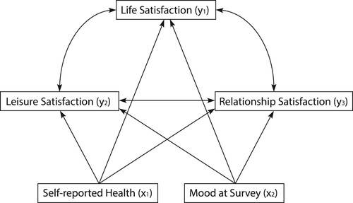
An important research question in Quality of Life research concerns how a person's satisfaction in certain life domains (e.g. about leisure, relationship, or work) relates to overall life satisfaction [16,53]. A prevailing hypothesis is that women are much more relational than men [23]. As these authors point out, women like being connected (i.e. experiencing ‘we-ness’), doing things together with others, and they place great emphasis on talking and emotional sharing. Men, on the other hand, see togetherness more as an activity than a state of being, as it is for women. They favor interactions that involve ‘doing’ rather than ‘being.’ Unlike women, men ‘prefer to have an element of separation included in their relationships with others and the ‘doing’ orientation seems to promote this’ [23, p. 465]. Research has furthermore shown that men have on average more leisure time than women [39]. Based on these general theoretical ideas and observations concerning gender differences in relational issues and leisure, we anticipate that such systematic differences will also be observed in how satisfaction with one's relationship and leisure is associated with overall life satisfaction, with leisure satisfaction relating more strongly to overall life satisfaction among men and relationship satisfaction relating more strongly to overall life satisfaction among women. Consider the following graphical model about the partial associations between three focal dependent variables that might be included in such an analysis: the degree of life satisfaction, leisure satisfaction, and relationship satisfaction (Figure 1). In this example we are interested in testing various informative hypotheses about conditional partial associations between the variables concerned, with gender also potentially moderating such partial associations. As can be seen, in this model the associations between the key variables of interest are controlled for differences in self-reported health and mood at survey.

Figure 1. Graphical model describing partial associations between life and domain satisfaction variables.

We use data from the Dutch LISS panel (Longitudinal Internet Studies for the Social sciences) to test various informative hypotheses about this model. In particular, the LISS panel contains the following variables used to operationalize the variables in the conceptual model:

1. Life Satisfaction ($y_1$): respondents were asked to rate the following statement: ‘I am satisfied with my life’; ordered categorical variable, with 1 = strongly disagree – 7 strongly agree

2. Leisure Satisfaction ($y_2$): respondents were asked to indicate how satisfied they are with the way in which they spend their leisure time; continuous variable, with 1 = entirely dissatisfied – 11 entirely satisfied

3. Relationship Satisfaction ($y_3$): respondents were asked to indicate how satisfied they are with their current relationship; continuous variable, with 1 = entirely dissatisfied – 11 entirely satisfied

4. Self-reported Health ($x_1$): respondents were asked: ‘How would you describe your health, generally speaking?’; ordered categorical variable, with 1 = poor – 5 = excellent

5. Mood at Survey ($x_2$): respondents were asked to indicate how they feel at the moment of completing the survey; ordered categorical variable, with 1 = very bad and 7 = very good

6. Gender (grouping variable g): the respondent's gender, with 1 = men and 2 = women

Several competing informative hypotheses can be formulated about the ordering of, and equalities between the partial correlations between $y_1$, $y_2$ and $y_3$ conditional on group g. Here, we consider the following hypothesis tests:

Hypothesis test 1 on the partial associations for men

Hypothesis $H_{1a}:$ The partial association between leisure satisfaction and life satisfaction is stronger than the partial association between relationship satisfaction and life satisfaction, and in turn this association is stronger than the partial association between leisure satisfaction and relationship satisfaction: $H_{1a}:{\rho }_{g1y2y1}>{\rho }_{g1y3y1}>{\rho }_{g1y3y2}.$ Hypothesis $H_{1b}:$ The partial association between relationship satisfaction and life satisfaction is stronger than the partial association between leisure satisfaction and life satisfaction, and in turn this association is stronger than the partial association between leisure satisfaction and relationship satisfaction: $H_{1b}:{\rho }_{g1y3y1}>{\rho }_{g1y2y1}>{\rho }_{g1y3y2}.$ Hypothesis $H_{1c}:$ The partial associations between life satisfaction, leisure satisfaction, and relationship satisfaction are equal: $H_{1c}:{\rho }_{g1y3y1}={\rho }_{g1y2y1}={\rho }_{g1y3y2}.$ Hypothesis $H_{1d}:$ The complement hypothesis, which implies that neither of the above three constrained hypotheses are true: $H_{1d}:`\mathrm{n}\mathrm{e}\mathrm{i}\mathrm{t}\mathrm{h}\mathrm{e}\mathrm{r}{H}_{1a},H_{1b},\mathrm{n}\mathrm{o}\mathrm{r}{H}_{1c}^{\prime }.$

Hypothesis test 2 on the partial associations for women

For the women (group 2) an equivalent hypothesis test is considered with equality or order constraints on the partial correlations $\begin{array}{rl}{H}_{2a}& :{\rho }_{g2y2y1}>{\rho }_{g2y3y1}>{\rho }_{g2y3y2}\\ H_{2b}& :{\rho }_{g2y3y1}>{\rho }_{g2y2y1}>{\rho }_{g2y3y2}\\ H_{2c}& :{\rho }_{g2y3y1}={\rho }_{g2y2y1}={\rho }_{g2y3y2}\\ H_{2d}& :`\mathrm{n}\mathrm{e}\mathrm{i}\mathrm{t}\mathrm{h}\mathrm{e}\mathrm{r}{H}_{2_a},H_{2_b},\mathrm{n}\mathrm{o}\mathrm{r}{H}_{2_c}^{\prime }.\end{array}$ Hypothesis test 3 on the partial associations between leisure satisfaction and life satisfaction with gender as moderator

Hypothesis $H_{3a}:$ The partial association between leisure satisfaction and life satisfaction among men is stronger than the partial association among women: $H_{3a}:{\rho }_{g1y2y1}>{\rho }_{g2y2y1}.$ Hypothesis $H_{3b}:$ The partial association between leisure satisfaction and life satisfaction among men is equally strong as the partial association among women: $H_{3b}:{\rho }_{g1y2y1}={\rho }_{g2y2y1}.$ Hypothesis $H_{3c}:$ The partial association between leisure satisfaction and life satisfaction among women is stronger than the partial association among men: $H_{3c}:{\rho }_{g1y2y1}<{\rho }_{g2y2y1}.$ Hypothesis test 4 on the partial associations between relationship satisfaction and life satisfaction with gender as moderator

Hypothesis $H_{4a}:$ The partial association between relationship satisfaction and life satisfaction among women is stronger than the partial association among men: $H_{4a}:{\rho }_{g2y3y1}>{\rho }_{g1y3y1}.$ Hypothesis $H_{4b}:$ The partial association between relationship satisfaction and life satisfaction among men is equally strong as the partial association among women: $H_{4b}:{\rho }_{g2y3y1}={\rho }_{g1y3y1}.$ Hypothesis $H_{4c}:$ The partial association between relationship satisfaction and life satisfaction among men is stronger than the partial association among women: $H_{4c}:{\rho }_{g2y3y1}<{\rho }_{g1y3y1}.$

2.2. Application 2: association between egalitarian justice beliefs across countries

Two important egalitarian norms that people can use in evaluating how societal resources (e.g. wealth, public goods) should be distributed are the principle of equality and the principle of need [12]. When people apply the equality principle, they support the idea that everyone should receive the same amount of such valuable societal resources. When people use the principle of need, they believe that societal resources should be distributed according to an individual's needs, for example the minimum resources required to lead a decent life.

As [62, p. 424] point out, the principles of need and equality are similar in their egalitarian belief and make that both justice principles are positively correlated [2]. Presumably, because of the legacy of the social system of communist regimes and ideological socialization within this system, people from these post-communist countries of Eastern Europe attach a more similar meaning to the equality and need principle than people from Western European countries. Thus the degree to which these justice principles are positively associated presumably varies between countries. In this respect, in Europe, a critical socio-historical divide exists between the Western European countries and the post-communist countries of Eastern Europe. In the context of communism, egalitarianism was the dominant ideology, and we can expect that citizens of former communist countries are only slowly abandoning strong endorsement of egalitarian beliefs even in the light of market reforms [62, p. 425]. Therefore, we expect that the correlation between both egalitarian justice principles will be stronger in post-communist countries than in Western European countries; this will hold even if in Western European countries public endorsement of the egalitarian ideology also has played an important role but within the context of a long-established capitalist market economy. Among the populations of capitalist Western European countries, presumably, equity or meritocratic considerations (i.e. assigning societal resources proportional to each's contributions or merits that deserve reward) also play a crucial role in deciding how societal resources should be distributed. Consequently, endorsement of egalitarian justice principles will be more fragmented in Western European countries which presumably results in weaker associations between the need and equality principle. Of course, even in Western European countries there is considerable difference in the degree to which egalitarian principles are institutionally embedded, with the Sweden being the model of the social-democratic welfare state. Finally, we expect that such differences in the strength of (partial) association between both egalitarian principles hold across countries, even if we control for variables such as gender, age and educational attainment, which relate to such justice principles [2].

We use data from the European Values Survey 2000 to test informative hypotheses about the presumed cross-national differences in the association between support for the equality and need principle. We limit our investigation to four countries that reflect the difference between post-communist countries and Western European capitalist countries with a more or less egalitarian ideology: Bulgaria, Romania, The Netherlands, and Sweden. We use the following variables:

1. ‘In order to be considered “just”, what should a society provide? Please tell me for each statement if it is important or unimportant to you.’

   Endorsement of the equality principle ($y_1$): ‘Eliminating big inequalities in income between citizens’; ordered categorical variable, with 1 = not at all important – 5 very important

   Endorsement of the need principle ($y_2$): ‘Guaranteeing that basic needs are met for all, in terms of food, housing, clothes, education, health’; ordered categorical variable, with 1 = not at all important – 5 very important

2. Gender ($x_1$): the respondent's gender, with 1 = men and 2 = women,

3. Age ($x_2$): the respondent's age in years

4. Education ($x_3$): age at which full-time education will or was completed (continuous variable with 11 intervals, ranging from 0 = no formal education to 10 = 21 and more years)

5. Country (grouping variable g): the respondent's country, with 1= Bulgaria, 2 = Romania, 3 = Sweden, and 4 = The Netherlands

Hypothesis test 5 on the partial associations with country as moderator

Hypothesis $H_{5a}:$ The partial association between support for the equality principle and the need principle is ordered as follows: it is strongest in Bulgaria, weaker in Romania (because of more violent resistance against communist rule and dictatorship in this country), even weaker in Sweden (Western European country with a strong egalitarian welfare ideology) and weakest in The Netherlands (a Western European country with a moderately egalitarian welfare ideology) : $H_{5a}:{\rho }_{g1y2y1}>{\rho }_{g2y2y1}>{\rho }_{g3y2y1}>{\rho }_{g4y2y1}$ Hypothesis $H_{5b}:$ The partial association between support for the equality principle and the need principle is equal between all countries: $H_{5b}:{\rho }_{g1y2y1}={\rho }_{g2y2y1}={\rho }_{g3y2y1}={\rho }_{g4y2y1}$ Hypothesis $H_{5c}:$ The partial association between support for the equality principle and the need principle is equal among post-communist countries Bulgaria and Romania, and the partial association between support for the equality principle and the need principle is equal among the Western European countries Netherlands and Sweden; however, the association between support for the equality principle and the need principle is stronger among post-communist countries than among Western European countries: $H_{5c}:{\rho }_{g1y2y1}={\rho }_{g2y2y1}>{\rho }_{g3y2y1}={\rho }_{g4y2y1}$ Hypothesis $H_{5d}:$ The complement hypothesis, i.e. $H_{5d}:`\mathrm{n}\mathrm{e}\mathrm{i}\mathrm{t}\mathrm{h}\mathrm{e}\mathrm{r}{H}_{5a},H_{5b},\mathrm{n}\mathrm{o}\mathrm{r}{H}_{5c}^{\prime }.$ The above hypothesis tests with equality and order constraints on measures of association will be executed in Section 6 using the Bayesian testing framework presented next.

3. Model specification and multiple constrained hypothesis test

3.1. The generalized multivariate probit model

The generalized multivariate probit model is very popular in the social and the behavioral sciences. It is a common framework for modeling combinations of continuous and ordinal outcome variables in professional software packages, such as Mplus [3] or Stata [63]. The Bayesian version of the model is also well-established in the Bayesian literature (e.g. [1,3,4,9–11,15,17,30,31,35,56]).

We consider a generalized multivariate probit model for G independent populations. In the first empirical application of the previous section for example there were G = 2 populations: a male population and a female population. The P-dimension vector of dependent variables in population g consists of $P_1$ normally distributed continuous variables and $P_2$ ordinal variables, such that $P=P_1+P_2$. The vector of standard deviations of the continuous variables in group g will be denoted by ${\mathit{\sigma }}_g$. By considering a multivariate normal distributed latent variable for the ordinal variables with (unknown) threshold parameters to define the ordinal categories, the dependent continuous and ordinal variables can be jointly modeled. Under group g, the correlation matrix of these variables will be denoted by ${\mathbf{C}}_g$ and the correlation between the pth and $p^{\prime }$th dependent variable will be denoted by ${\rho }_{gp{p}^{\prime }}$. It is possible to control for certain variables (e.g. Mood at Survey in Application 1) by including them as covariates in the model. In this case we would model partial correlations. The matrix of regression coefficients of these covariates under group g will be denoted by ${\mathbf{B}}_g$. The mathematical details of the model can be found in Appendix 1.

3.2. Hypothesis testing on measures of association

In the context of testing constraints on correlations, which is the goal of the current paper, the correlation matrices ${\mathbf{C}}_g$ are of central importance while the parameter matrix ${\mathbf{B}}_g$ and the variances $\mathit{\sigma }$ are treated as nuisance parameters. The correlations in ${\mathbf{C}}_g$ are contained in the vector $\mathit{\rho }$, e.g. (1) $\begin{array}{r}{\mathbf{C}}_g=\left[\begin{array}{c}1\\ {\rho }_{g21}& 1\\ {\rho }_{g31}& {\rho }_{g32}& 1\end{array}\right]\Rightarrow {\mathit{\rho }}_g=({\rho }_{g21},{\rho }_{g31},{\rho }_{g32}{)}^{\prime }.\end{array}$(1) Furthermore, all correlations in the G different correlation matrices, ${\mathbf{C}}_g$, will be combined in the vector ${\mathit{\rho }}^{\prime }=({\mathit{\rho }}_1^{\prime },\dots ,{\mathit{\rho }}_G^{\prime })$ of length $L=\frac{1}{2}GP(P-1)$. Similarly we combine the parameter matrices ${\mathbf{B}}_g$ and variances ${\mathit{\sigma }}_g$ over all G population in the matrices $\mathbf{B}$ and $\mathit{\sigma }$, respectively, and subsequently, the vectorization of $\mathbf{B}$ is denoted by the vector $\text{β}$.

We consider a multiple hypothesis test of T hypotheses $H_1,\dots ,H_T$ of the form (2) $H_t:{\mathbf{R}}_t^E\mathit{\rho }={\mathbf{r}}_t^E,{\mathbf{R}}_t^I\mathit{\rho }>{\mathbf{r}}_t^I,$(2) for $t=1,\dots ,T$, where $\left[{\mathbf{R}}_t^E|{\mathbf{r}}_t^E\right]$ is a matrix of coefficients that capture the set of equality constraints under $H_t$ and $\left[{\mathbf{R}}_t^I|{\mathbf{r}}_t^I\right]$ is a matrix of coefficients that capture the set of inequality (or order) constraints under $H_t$. We shall focus on the problem which hypothesis receives most evidence from the data.

In most applications researchers either compare two correlations with each other, e.g. ${\rho }_{121}>{\rho }_{131}$, or a single correlation is compared to constant, e.g. ${\rho }_{121}>.5$. Therefore each row of the matrices $\left[{\mathbf{R}}_t^E\right]$ and $\left[{\mathbf{R}}_t^I\right]$ is either a permutation of $(1,-1,0\dots ,0)$ with corresponding constant in ${\mathbf{r}}_t^E$ and ${\mathbf{r}}_t^I$ equals 0, or a row is a permutation of $(\pm 1,0,\dots ,0)$ with corresponding constant $r\in (-1,1)$. As an example, hypothesis $H_{1_a}:{\rho }_{121}>{\rho }_{131}>{\rho }_{132}$ from Section 2.1 (with the index labels omitted) would have the following matrix form ${\mathit{H}\mathbf{1}}_a:\left[\begin{array}{cccccc}1& -1& 0& 0& 0& 0\\ 0& 1& -1& 0& 0& 0\end{array}\right]\left[\begin{array}{c}{\rho }_{121}\\ {\rho }_{131}\\ {\rho }_{132}\\ {\rho }_{221}\\ {\rho }_{231}\\ {\rho }_{232}\end{array}\right]>\left[\begin{array}{c}0\\ 0\end{array}\right].$ Throughout the paper the allowed parameter space under the constrained $H_t$ will be denoted by ${\mathcal{C}}_t$. In certain parts of the paper we refer to an unconstrained hypothesis, denoted by $H_u$, which does not assume any constraints on the correlations besides the necessary constraints on $\mathit{\rho }$ that ensure that the corresponding correlation matrices are positive definite.

4. Statistical methodology for Bayes factor testing on measures of association

Bayes factors are known to be sensitive to the choice of the prior, and therefore the prior needs to be carefully specified. The specification of the prior becomes increasingly complex in the current setting when testing multiple statistical hypotheses with different configurations of the equality, one-sided, and order constraints on measures of association. In this section we propose a class of constrained joint uniform priors on the measures of association which assume that all combinations of values of the correlations in the correlation matrices are equally likely a priori under a given constrained hypothesis. We explain how this class of priors may be preferred over other choices which have been considered in the literature. Because these constrained priors are in fact truncations of the same unconstrained prior, it is possible to formulate the Bayes factor of each constrained hypothesis against the unconstrained hypothesis using an extended formulation of the Savage–Dickey density ratio. The advantage of this expression is that marginal likelihood computation, which can be computationally expensive, can be avoided. Before discussing these contributions we start with some background and terminology on Bayes factors and posterior probabilities for statistical hypotheses.

4.1. Background on Bayes factors and posterior probabilities

The Bayes factor is a Bayesian criterion that quantifies the relative evidence in the data between two hypotheses. The Bayes factor of hypothesis $H_1$ versus $H_2$ is defined by the ratio of the marginal likelihoods under the respective hypotheses, i.e. (3) $B_{12}=\frac{m_1\left(\mathbf{Y}\right)}{m_2\left(\mathbf{Y}\right)},$(3) where the marginal likelihood is defined by (4) $m_t\left(\mathbf{Y}\right)={\iiint }_{{\mathcal{C}}_t}{p}_t(\mathbf{Y}|\mathbf{X},\text{β},\mathit{\sigma },\mathit{\rho }){\pi }_t(\text{β},\mathit{\sigma },\mathit{\rho })\mathrm{d}\mathit{\rho }\mathrm{d}\mathit{\sigma }\mathrm{d}\text{β},$(4) where $p_t$ denotes the likelihood of the data $\mathbf{Y}$ given the unknown parameters and the covariates $\mathbf{X}$ under $H_t$, which follows directly from (A1(A1) $\begin{array}{rl}\left[\begin{array}{c}{\mathbf{v}}_{ig}\\ {\mathbf{z}}_{ig}\end{array}\right]& \sim N({\mathbf{B}}_g{\mathbf{x}}_{ig},{\mathbf{\Sigma }}_g),\text{where}\end{array}$(A1) ) and (A2(A2) $\begin{array}{rl}{\mathbf{\Sigma }}_g& =\text{diag}({\mathit{\sigma }}_g^{\prime },{\mathbf{1}}_{P_2}^{\prime }){\mathbf{C}}_g\text{diag}({\mathit{\sigma }}_g^{\prime },{\mathbf{1}}_{P_2}^{\prime }),\end{array}$(A2) ), and ${\pi }_t$ denotes the prior for the unknown model parameters under $H_t$. The prior reflects the plausibility of the possible values of the free parameters before observing the data. The marginal likelihood captures how likely the observed data is under a hypothesis and its respective prior.

One of the main strengths of the Bayes factor is its intuitive interpretation. For example, the Bayes factor is symmetrical in the sense that if, say $B_{12}=.1$, which implies that $H_1$ receives 10 times less evidence than $H_2$, it follows naturally from (3(3) $B_{12}=\frac{m_1\left(\mathbf{Y}\right)}{m_2\left(\mathbf{Y}\right)},$(3) ) that $B_{21}=B_{12}^{-1}=10$, which implies that $H_2$ receives 10 times more evidence from the data than $H_1$. Furthermore, Bayes factors are transitive in the sense that if $H_1$ received 10 times more evidence than $H_2$, i.e. $B_{12}=10$, and $H_2$ received 5 times more evidence than $H_3$, i.e. $B_{32}=5$, it again follow naturally from the definition in (3(3) $B_{12}=\frac{m_1\left(\mathbf{Y}\right)}{m_2\left(\mathbf{Y}\right)},$(3) ) that hypothesis $H_1$ received 50 times more evidence than $H_3$ because $B_{13}=B_{12}\times B_{23}=10\times 5=50$.

Various researchers have provided an indication how to interpret Bayes factors (e.g. [24,57]). For completeness we provided the guidelines that were given by Raftery [57] in Table 3. These guidelines are helpful for researchers who are new to Bayes factors. We do not recommend to use these guidelines as strict rules because researchers should decide by himself or herself when he or she feels that the Bayes factor indicates strong evidence.

Table 3. Rough guidelines for interpreting Bayes factors [57].

$B_{12}$	Evidence
$<1/150$	Very strong evidence for $H_2$
1/150 to 1/20	Strong evidence for $H_2$
1/20 to 1/3	Positive evidence for $H_2$
1/3 to 1	Weak evidence for $H_2$
1	No preference
1 to 3	Weak evidence for $H_1$
3 to 20	Positive evidence for $H_1$
20 to 150	Strong evidence for $H_1$
$>150$	Very strong evidence for $H_1$

The Bayes factor can be used to update the prior odds of any pair two hypotheses that can be true before observing the data to obtain the posterior odds that the hypotheses are true after observing the data according to (5) $\frac{\text{Pr}\left(H_1|\mathbf{Y}\right)}{\text{Pr}\left(H_2|\mathbf{Y}\right)}=B_{12}\times \frac{\text{Pr}\left(H_1\right)}{\text{Pr}\left(H_2\right)},$(5) where $\text{Pr}\left(H_t\right)$ and $\text{Pr}\left(H_2|\mathbf{Y}\right)$ denote the prior and posterior probability that $H_t$ is true, respectively, for t = 1 or 2. In the general case of T hypotheses, the posterior hypothesis probabilities can be obtained as follows (6) $\text{Pr}\left(H_t|\mathbf{Y}\right)=\frac{\text{Pr}\left(H_t\right)B_{t1}}{\sum _{t^{\prime }=1}^T\text{Pr}\left(H_{t^{\prime }}\right)B_{t^{\prime }1}}.$(6) Posterior hypothesis probabilities are useful because they provide a direct answer to the research question how plausible each hypothesis is in light of the observed data. Researchers typically find these posterior probabilities easier to interpret than Bayes factors. It should be noted however that in the case of equal prior probabilities for the hypotheses, i.e. $\text{Pr}\left(H_1\right)=\text{Pr}\left(H_2\right)$, which is the default setting, the posterior odds between two hypotheses corresponds exactly to the respective Bayes factor as can be seen in (5(5) $\frac{\text{Pr}\left(H_1|\mathbf{Y}\right)}{\text{Pr}\left(H_2|\mathbf{Y}\right)}=B_{12}\times \frac{\text{Pr}\left(H_1\right)}{\text{Pr}\left(H_2\right)},$(5) ).

4.2. Priors for measures of association under constrained hypotheses

4.2.1. Constrained joint uniform priors

Under each hypothesis, we set independent priors for the three different types of model parameters, i.e. (7) ${\pi }_t(\text{β},\mathit{\sigma },\mathit{\rho })={\pi }_t^N\left(\text{β}\right)\times {\pi }_t^N\left(\mathit{\sigma }\right)\times {\pi }_t^U\left(\mathit{\rho }\right)\times I(\mathit{\rho }\in {\mathcal{C}}_t),$(7) with noninformative improper priors for the nuisance parameters (8) $\begin{array}{rl}{\pi }_t^N\left(\text{β}\right)& \propto 1\end{array}$(8) (9) $\begin{array}{rl}{\pi }_t^N\left(\mathit{\sigma }\right)& \propto \prod _{g=1}^G{\sigma }_{g,1}^{-1}\times \dots \times {\sigma }_{g,P_1}^{-1}.\end{array}$(9) The domains for $\text{β}$ for $\mathit{\sigma }$ are ${\mathbb{R}}^{PQ}$ and $({\mathbb{R}}^{+}{)}^P$, respectively. Note that the priors for the nuisance parameters are equivalent to independent Jeffreys priors which are commonly used for default Bayesian analyses. These noninformative improper priors are allowed for these common nuisance parameters as the Bayes factor will be virtually independent to the exact choice of these priors as long as the priors are vaguely enough. This will be explained later in this paper.

It is well known that proper priors (i.e. prior distributions that integrate to one) need to be formulated for the parameters that are tested, i.e. the correlations, in order for the Bayes factor to be well-defined. In this paper we consider a uniform prior for the correlations under a hypothesis in its allowed constrained subspace. This implies that every combination of values for the correlations that satisfies the constraints is equally likely a priori under each hypothesis. The prior for $\mathit{\rho }$ is zero outside the constrained subspace under each hypothesis. Because the constrained parameter space ${\mathcal{C}}_t$ is bounded, a proper uniform prior can be formulated for the correlations under every hypothesis, i.e. (10) ${\pi }_t^U\left(\mathit{\rho }\right)=V_t^{-1}\times I(\mathit{\rho }\in {\mathcal{C}}_t),$(10) where the normalizing constant $V_t$ is given by (11) $V_t={\int }_{{\mathcal{C}}_t}1\mathrm{d}\mathit{\rho }.$(11) The normalizing constant $V_t$ can be seen as a measure of the size or volume of the constrained space.

To illustrate the priors under different constrained hypotheses on measures, let us consider a model with 3 dependent variables and one population (the correlation matrix was given in (1(1) $\begin{array}{r}{\mathbf{C}}_g=\left[\begin{array}{c}1\\ {\rho }_{g21}& 1\\ {\rho }_{g31}& {\rho }_{g32}& 1\end{array}\right]\Rightarrow {\mathit{\rho }}_g=({\rho }_{g21},{\rho }_{g31},{\rho }_{g32}{)}^{\prime }.\end{array}$(1) ) where we omit the population index j). Furthermore, let us consider the following hypotheses:

• $H_u:{\rho }_{21},{\rho }_{31},{\rho }_{32}$ (the unconstrained hypothesis).

• $H_1:{\rho }_{21}={\rho }_{31}={\rho }_{32}$ (all ρ's are equal).

• $H_2:{\rho }_{31}=0,{\rho }_{21},{\rho }_{32}$ (only ${\rho }_{31}$ is restricted to zero).

• $H_3:{\rho }_{31}=0,{\rho }_{21}>{\rho }_{32}$ (${\rho }_{31}$ is restricted to zero and ${\rho }_{21}$ is larger than ${\rho }_{32}$).

The unconstrained parameter space of $\mathit{\rho }=({\rho }_{21},{\rho }_{31},{\rho }_{32}{)}^{\prime }$ that results in a positive definite correlation matrix is displayed in Figure 2(a) (taken from [59] with permission). As noted by Joe [25], the volume of this 3-dimensional subspace equals 4.934802. Therefore, the volume under the unconstrained hypothesis $H_u$ is given by $V_u=4.934802$ in (11(11) $V_t={\int }_{{\mathcal{C}}_t}1\mathrm{d}\mathit{\rho }.$(11) ). Therefore, the unconstrained uniform prior for the correlations equals ${\pi }_u^U\left(\mathit{\rho }\right)=\frac{1}{4.934802}\times I(\mathit{\rho }\in {\mathcal{C}}_u)$ in (10(10) ${\pi }_t^U\left(\mathit{\rho }\right)=V_t^{-1}\times I(\mathit{\rho }\in {\mathcal{C}}_t),$(10) ).

Figure 2. (a) Graphical representation of the subspace of $({\rho }_{21},{\rho }_{31},{\rho }_{32})$ for which the 3-dimensional correlation matrix is positive definite (taken from [59] with permission). The thick diagonal line from $(-\frac{1}{2},-\frac{1}{2},-\frac{1}{2})$ to $(1,1,1)$ represents the correlations that satisfy ${\rho }_{21}={\rho }_{31}={\rho }_{32}$ and result in a positive diagonal correlation matrix. (b) Uniform prior ${\pi }_1^U$ for the common correlation ρ under $H_1:{\rho }_{21}={\rho }_{31}={\rho }_{32}$ in the allowed region ${\mathcal{C}}_1=\{\rho |\rho \in (-\frac{1}{2},1\left)\right\}$. (c) Uniform prior ${\pi }_2^U$ for the free parameters under $H_2:{\rho }_{31}=0$ in the allowed region ${\mathcal{C}}_2=\left\{\right({\rho }_{21},{\rho }_{32})|{\rho }_{21}^2+{\rho }_{32}^2<1\}$. (d) Uniform prior for the free correlations under $H_3:{\rho }_{31}=0,{\rho }_{21}>{\rho }_{32}$ in the allowed region ${\mathcal{C}}_3=\left\{\right({\rho }_{21},{\rho }_{32})|{\rho }_{21}^2+{\rho }_{32}^2<1,{\rho }_{21}>{\rho }_{32}\}$.

When all ρ's are equal as under $H_1$, the common correlation, say, ρ, must lie in the interval $(-\frac{1}{2},1)$ to ensure positive definiteness (e.g. [45]). Thus, the size of the parameter space of ρ corresponds to the length of the interval which is $V_1=\frac{3}{2}$. Therefore, the uniform prior for ρ under $H_1$ corresponds to ${\pi }_1^U\left(\rho \right)=\frac{2}{3}\times I(\rho \in (-\frac{1}{2},1\left)\right)$, which is plotted in Figure 2(b). The diagonal ${\rho }_{21}={\rho }_{31}={\rho }_{32}$ is also plotted in Figure 2(a) as a dashed line, where the thick part lies within positive definite subspace ${\mathcal{C}}_u$.

When ${\rho }_{31}$ is restricted to zero as under $H_2$, the allowed parameter space for $({\rho }_{21},{\rho }_{32})$ that results in a positive definite correlation matrix must satisfy ${\rho }_{21}^2+{\rho }_{32}^2<1$, i.e. a circle with radius 1 [59]. Therefore, the uniform prior under $H_2:{\rho }_{31}=0$ is given by ${\pi }_2({\rho }_{21},{\rho }_{32})=\frac{1}{\pi }\times I({\rho }_{21}^2+{\rho }_{32}^2<1)$ (Figure 2(c)) because a circle or radius 1 has a surface of $V_2=\pi$.

When ${\rho }_{31}$ is restricted to zero and ${\rho }_{21}$ is larger than ${\rho }_{32}$ as under $H_3$, the subspace is half as small as under $H_2$. Therefore the uniform prior density for the free parameters under $H_3$ is twice as large as the prior under $H_1$ to ensure the prior integrates to one. Thus, the uniform prior under $H_3$ is given by ${\pi }_3({\rho }_{21},{\rho }_{32})=\frac{2}{\pi }\times I({\rho }_{21}^2+{\rho }_{32}^2<1\mathrm{\&}{\rho }_{21}>{\rho }_{32})$ (Figure 2(d)).

4.2.2. Comparison with other priors from the literature

Scale mixtures of g priors

Wetzels and Wagenmakers [68] proposed a test for a single bivariate or partial correlation, $H_0:\rho =0$ against $H_1:\rho \ne 0$, via a scale mixture of g priors [32,58,69]. Their test is formulated under a linear regression model $y_i={\text{β}}_0+{\text{β}}_1{x}_i+{ϵ}_i$, such that the hypothesis test is equivalent to testing $H_0:{\text{β}}_1=0$ against $H_1:{\text{β}}_1\ne 0$ where ρ is the correlation between Y and X. Under the alternative hypothesis, a g prior [70] is specified for β with an inverse gamma mixing prior for g. It can be shown (Appendix 1) that this prior is equivalent to a $beta(\frac{1}{2},\frac{1}{2})$ prior in the interval $(-1,1)$ for ρ (left panel of Figure 3; dotted line). As can be seen this prior puts most probability mass in the extreme regions near $-1$ and 1. For this reason this Bayes factor will result in an overestimation of the evidence in favor of $H_0$ because it assumes unrealistically large correlations to be most plausible under the alternative hypothesis. The uniform prior for ρ (left panel of Figure 3; solid line) on the other hand seems a better operationalization of ‘prior ignorance’ because it assumes that all correlations under the alternative are equally likely a priori.

Figure 3. Left panel. The implied $beta(\frac{1}{2},\frac{1}{2})$ prior in the interval $(-1,1)$ (dotted line) in the test proposed by Wetzels and Wagenmakers' [68], and the uniform prior in $(-1,1)$ as proposed here. Right panel. Implied prior for the common correlation ρ under $H_0:{\rho }_{12}={\rho }_{13}={\rho }_{23}$ when testing against $H_1:{\rho }_{12}\ne {\rho }_{13}\ne {\rho }_{23}$ using a marginally uniform encompassing prior (dotted line), and a uniform prior for ρ on $(-\frac{1}{2},1)$ (solid line) as proposed here.

Marginally uniform priors

Barnard et al. [4] showed how to construct a prior for a correlation matrix having uniform marginal priors for the separate bivariate correlations. For a $P\times P$ correlation matrix, this can simply be achieved by placing an inverse Wishart prior on the covariance matrix with an identity scale matrix and P + 1 degrees of freedom. Although the prior is very reasonable for Bayesian estimation (as shown by Barnard et al.), this marginally uniform prior distribution may not be reasonable as an encompassing prior when testing hypotheses with equality constraints on the correlations. To construct a prior that has uniformly distributed marginal priors for the separate correlations, most probability mass needs to be placed near the extremes (see Figure 2 of [4]). This will result in unrealistic priors for correlations under equality constrained hypotheses. As an example consider a hypothesis test of $H_0:{\rho }_{12}={\rho }_{13}={\rho }_{23}$ against $H_1:{\rho }_{12}\ne {\rho }_{13}\ne {\rho }_{23}$, and let us construct a prior for the common correlation $\rho ={\rho }_{12}={\rho }_{13}={\rho }_{23}$ under $H_0$ that is proportional to a marginally uniform encompassing prior. This yields a prior that is proportional to ${\pi }_0\left(\rho \right)\propto (2\rho +1)(1-\rho {)}^{-5/2}(\rho +1{)}^{-9/2}$ in the interval $(-\frac{1}{2},1)$ (Appendix 1), which is plotted in the right panel of Figure 3 (dotted line). This implied prior is concentrated near 1 which does not correspond to reasonable prior beliefs under $H_0$. Therefore a marginally uniform prior is not recommendable as default encompassing prior for testing hypotheses with equality constraints on the correlations. A uniform prior on $(-\frac{1}{2},1)$ would be a better default choice (solid line).

Note that [44] suggested a similar prior based on P degrees of freedom when testing order-constrained hypotheses and one-sided hypotheses on correlations. This results corresponds in $beta(\frac{1}{2},\frac{1}{2})$-distributed marginal priors in the interval $(-1,1)$ for the separate correlations [4]. Even though this may seem to be an unrealistic prior (as noted earlier), the Bayes factor is quite insensitive to the prior when testing order hypotheses because the Jeffreys-Lindley-Bartlett paradox does not play a role [42]. The use of a vague prior based on the minimal of P degrees of freedom would actually be preferably as it would result in least prior shrinkage.

4.3. The extended Savage–Dickey density ratio

In order to compute the marginal likelihood under each constrained hypothesis via (4(4) $m_t\left(\mathbf{Y}\right)={\iiint }_{{\mathcal{C}}_t}{p}_t(\mathbf{Y}|\mathbf{X},\text{β},\mathit{\sigma },\mathit{\rho }){\pi }_t(\text{β},\mathit{\sigma },\mathit{\rho })\mathrm{d}\mathit{\rho }\mathrm{d}\mathit{\sigma }\mathrm{d}\text{β},$(4) ) using the constrained uniform prior in (13(13) ${\pi }_u^U(\text{β},\mathit{\sigma },\mathit{\rho })=V_u^{-1}\times {\sigma }_{1,1}^{-1}\times \dots \times {\sigma }_{1,P_1}^{-1}\times I(\mathit{\rho }\in {\mathcal{C}}_u),$(13) ) a complex multivariate integral must be solved. This endeavor can be somewhat simplified by using the fact that the uniform prior for the correlations under each hypothesis $H_t$ can be written as a truncation of a uniform unconstrained prior under the unconstrained hypothesis $H_u$, i.e. (12) ${\pi }_t^U(\text{β},\mathit{\sigma },\mathit{\rho })=\frac{V_u}{V_t}\times {\pi }_u^U(\text{β},\mathit{\sigma },\mathit{\rho })\times I(\mathit{\rho }\in {\mathcal{C}}_t)$(12) where the unconstrained prior is given by (13) ${\pi }_u^U(\text{β},\mathit{\sigma },\mathit{\rho })=V_u^{-1}\times {\sigma }_{1,1}^{-1}\times \dots \times {\sigma }_{1,P_1}^{-1}\times I(\mathit{\rho }\in {\mathcal{C}}_u),$(13) where $V_u={\int }_{{\mathcal{C}}_u}1\mathrm{d}\mathit{\rho }$, which can be interpreted as the volume of the subspace of $\mathit{\rho }$ that results in positive definite correlation matrices under all populations. Note that the normalizing constant in (12(12) ${\pi }_t^U(\text{β},\mathit{\sigma },\mathit{\rho })=\frac{V_u}{V_t}\times {\pi }_u^U(\text{β},\mathit{\sigma },\mathit{\rho })\times I(\mathit{\rho }\in {\mathcal{C}}_t)$(12) ) is equal to the reciprocal of the unconstrained prior integrated over the constrained space ${\mathcal{C}}_t$, (14) ${\int }_{{\mathcal{C}}_t}{\pi }_u^U\left(\mathit{\rho }\right)\mathrm{d}\mathit{\rho }=V_u^{-1}{\int }_{{\mathcal{C}}_t}1\mathrm{d}\mathit{\rho }=\frac{V_t}{V_u}.$(14) This relationship between each constrained prior and the unconstrained prior allows us to use the following general result for computing the Bayes factor of a hypothesis with certain constraints on the parameters of interest against a larger unconstrained hypothesis in which the constrained hypothesis is nested.

Lemma 4.1

Consider a model where a hypothesis is formulated with equality and inequality constraints on the parameter vector $\mathit{\rho }$ of length Q of the form $H_t:{\mathbf{R}}_t^E\mathit{\rho }={\mathbf{r}}_t^E,{\mathbf{R}}_t^I\mathit{\rho }>{\mathbf{r}}_t^I$, where the $q^E\times Q$ matrix ${\mathbf{R}}_t^E$ has rank $q^E\le Q$, and a larger ‘unconstrained’ hypothesis $H_u$ in which $H_q$ is nested. Let the vector of nuisance parameters in the model are denoted by $\mathit{\varphi }$. If the prior of $\mathit{\rho }$ under $H_t$ is defined as the truncation of a proper prior for $\mathit{\rho }$ under $H_u$ in its constrained subspace, i.e. ${\pi }_t\left(\mathit{\rho }\right)\propto {\pi }_u\left(\mathit{\rho }\right)I(\mathit{\rho }\in {\mathcal{C}}_t)$, then the Bayes factor of $H_t$ against $H_u$ can be written as (15) $B_{tu}=\frac{\text{Pr}({\tilde{\mathbf{R}}}_t^I{\mathit{\rho }}_t^I>{\mathbf{r}}_t^I|{\mathit{\rho }}_t^E={\mathbf{r}}_t^E,H_u,\mathbf{Y},\mathbf{X})}{\text{Pr}({\tilde{\mathbf{R}}}_t^I{\mathit{\rho }}_t^I>{\mathbf{r}}_t^I|{\mathit{\rho }}_t^E={\mathbf{r}}_t^E,H_u)}\times \frac{{\pi }_u({\mathit{\rho }}_t^E={\mathbf{r}}_t^E|\mathbf{Y},\mathbf{X})}{{\pi }_u({\mathit{\rho }}_t^E={\mathbf{r}}_t^E)},$(15) where ${\mathit{\rho }}_t^E={\mathbf{R}}_t^E\mathit{\rho }$, ${\mathit{\rho }}_t^I$ are the elements of $\mathit{\rho }$ that are not restricted with equality constraints under $H_t$, and ${\tilde{\mathbf{R}}}_t^I$ consists of the columns of ${\mathbf{R}}_t^I$ such that ${\tilde{\mathbf{R}}}_t^I{\mathit{\rho }}_t^I={\mathbf{R}}_t^I\mathit{\rho }$.

Proof.

The derivation is a combined result of [13,19,28,55,67]. A proof is given in Appendix 2.

Note that the second factor in (15(15) $B_{tu}=\frac{\text{Pr}({\tilde{\mathbf{R}}}_t^I{\mathit{\rho }}_t^I>{\mathbf{r}}_t^I|{\mathit{\rho }}_t^E={\mathbf{r}}_t^E,H_u,\mathbf{Y},\mathbf{X})}{\text{Pr}({\tilde{\mathbf{R}}}_t^I{\mathit{\rho }}_t^I>{\mathbf{r}}_t^I|{\mathit{\rho }}_t^E={\mathbf{r}}_t^E,H_u)}\times \frac{{\pi }_u({\mathit{\rho }}_t^E={\mathbf{r}}_t^E|\mathbf{Y},\mathbf{X})}{{\pi }_u({\mathit{\rho }}_t^E={\mathbf{r}}_t^E)},$(15) ) is equal to the well-known Savage–Dickey density ratio [13,66,67]. The ratio of posterior and prior probabilities in the first factor was also observed in [28] when there are no equality constraints under $H_t$. The conditional posterior probability, i.e. the numerator of the first term of (15(15) $B_{tu}=\frac{\text{Pr}({\tilde{\mathbf{R}}}_t^I{\mathit{\rho }}_t^I>{\mathbf{r}}_t^I|{\mathit{\rho }}_t^E={\mathbf{r}}_t^E,H_u,\mathbf{Y},\mathbf{X})}{\text{Pr}({\tilde{\mathbf{R}}}_t^I{\mathit{\rho }}_t^I>{\mathbf{r}}_t^I|{\mathit{\rho }}_t^E={\mathbf{r}}_t^E,H_u)}\times \frac{{\pi }_u({\mathit{\rho }}_t^E={\mathbf{r}}_t^E|\mathbf{Y},\mathbf{X})}{{\pi }_u({\mathit{\rho }}_t^E={\mathbf{r}}_t^E)},$(15) ), can be interpreted as a measure of fit of the order constraints of $H_t$ relative to $H_u$; the marginal posterior density, i.e. the numerator of the second term of (15(15) $B_{tu}=\frac{\text{Pr}({\tilde{\mathbf{R}}}_t^I{\mathit{\rho }}_t^I>{\mathbf{r}}_t^I|{\mathit{\rho }}_t^E={\mathbf{r}}_t^E,H_u,\mathbf{Y},\mathbf{X})}{\text{Pr}({\tilde{\mathbf{R}}}_t^I{\mathit{\rho }}_t^I>{\mathbf{r}}_t^I|{\mathit{\rho }}_t^E={\mathbf{r}}_t^E,H_u)}\times \frac{{\pi }_u({\mathit{\rho }}_t^E={\mathbf{r}}_t^E|\mathbf{Y},\mathbf{X})}{{\pi }_u({\mathit{\rho }}_t^E={\mathbf{r}}_t^E)},$(15) ), can be seen as a measure of fit of the equality constraints of $H_t$ relative to $H_u$; the conditional prior probability, i.e. the denominator of the first term of (15(15) $B_{tu}=\frac{\text{Pr}({\tilde{\mathbf{R}}}_t^I{\mathit{\rho }}_t^I>{\mathbf{r}}_t^I|{\mathit{\rho }}_t^E={\mathbf{r}}_t^E,H_u,\mathbf{Y},\mathbf{X})}{\text{Pr}({\tilde{\mathbf{R}}}_t^I{\mathit{\rho }}_t^I>{\mathbf{r}}_t^I|{\mathit{\rho }}_t^E={\mathbf{r}}_t^E,H_u)}\times \frac{{\pi }_u({\mathit{\rho }}_t^E={\mathbf{r}}_t^E|\mathbf{Y},\mathbf{X})}{{\pi }_u({\mathit{\rho }}_t^E={\mathbf{r}}_t^E)},$(15) ), can be interpreted as a measure of complexity of the order constraints of $H_t$ relative to $H_u$; the marginal prior density, i.e. the denominator of the second term of (15(15) $B_{tu}=\frac{\text{Pr}({\tilde{\mathbf{R}}}_t^I{\mathit{\rho }}_t^I>{\mathbf{r}}_t^I|{\mathit{\rho }}_t^E={\mathbf{r}}_t^E,H_u,\mathbf{Y},\mathbf{X})}{\text{Pr}({\tilde{\mathbf{R}}}_t^I{\mathit{\rho }}_t^I>{\mathbf{r}}_t^I|{\mathit{\rho }}_t^E={\mathbf{r}}_t^E,H_u)}\times \frac{{\pi }_u({\mathit{\rho }}_t^E={\mathbf{r}}_t^E|\mathbf{Y},\mathbf{X})}{{\pi }_u({\mathit{\rho }}_t^E={\mathbf{r}}_t^E)},$(15) ), can be seen as a measure of complexity based on the equality constraints of $H_t$ relative to $H_u$; see also [19,42]. Evaluating equality constraints and the inequality constraints conditional on the equality constraints separately was shown by [55]. The contribution here is that the Bayes factor is derived for the general case of a set of linear equality constraints and a set of linear inequality constraints where the prior under $H_t$ is a truncation of a proper unconstrained prior. A similar result was derived for (adjusted) fractional Bayes factors by [19,49].

In the current paper, the nuisance parameters $\mathit{\varphi }$ correspond to the vector of the elements $\mathbf{B}$ and $\mathit{\sigma }$. Expression (15(15) $B_{tu}=\frac{\text{Pr}({\tilde{\mathbf{R}}}_t^I{\mathit{\rho }}_t^I>{\mathbf{r}}_t^I|{\mathit{\rho }}_t^E={\mathbf{r}}_t^E,H_u,\mathbf{Y},\mathbf{X})}{\text{Pr}({\tilde{\mathbf{R}}}_t^I{\mathit{\rho }}_t^I>{\mathbf{r}}_t^I|{\mathit{\rho }}_t^E={\mathbf{r}}_t^E,H_u)}\times \frac{{\pi }_u({\mathit{\rho }}_t^E={\mathbf{r}}_t^E|\mathbf{Y},\mathbf{X})}{{\pi }_u({\mathit{\rho }}_t^E={\mathbf{r}}_t^E)},$(15) ) shows that the Bayes factor for a constrained hypothesis against the unconstrained hypothesis only depends on the prior for the nuisance parameters through the unconstrained marginal posterior of the correlations $\mathit{\rho }$, i.e. ${\pi }_u(\mathit{\rho }|\mathbf{Y},\mathbf{X})=\iint {\pi }_u(\mathit{\rho }|\mathbf{B},\mathit{\sigma },\mathbf{Y},\mathbf{X})\times {\pi }_u(\mathbf{B},\mathit{\sigma }|\mathbf{Y},\mathbf{X})\mathrm{d}\mathbf{B}\mathrm{d}\mathit{\sigma },$ where ${\pi }_u(\mathbf{B},\mathit{\sigma }|\mathbf{Y},\mathbf{X})\propto \int p(\mathbf{Y}|\mathbf{X},\mathbf{B},\mathit{\sigma },\mathit{\rho })\times {\pi }_u^N\left(\mathbf{B}\right)\times {\pi }_u^N\left(\mathit{\sigma }\right)\times {\pi }_u\left(\mathit{\rho }\right)\mathrm{d}\mathit{\rho }.$ As is well-known from Bayesian estimation, if different vague priors would have been specified for $\mathbf{B}$ and $\mathit{\sigma }$, e.g. a vague matrix-normal prior or inverse gamma prior, respectively, the unconstrained posterior for $\mathbf{B}$ and $\mathit{\sigma }$ would have been virtually the same, and thus, the marginal posterior for $\mathit{\rho }$ would have been virtually the same. Therefore, the Bayes factor in (15(15) $B_{tu}=\frac{\text{Pr}({\tilde{\mathbf{R}}}_t^I{\mathit{\rho }}_t^I>{\mathbf{r}}_t^I|{\mathit{\rho }}_t^E={\mathbf{r}}_t^E,H_u,\mathbf{Y},\mathbf{X})}{\text{Pr}({\tilde{\mathbf{R}}}_t^I{\mathit{\rho }}_t^I>{\mathbf{r}}_t^I|{\mathit{\rho }}_t^E={\mathbf{r}}_t^E,H_u)}\times \frac{{\pi }_u({\mathit{\rho }}_t^E={\mathbf{r}}_t^E|\mathbf{Y},\mathbf{X})}{{\pi }_u({\mathit{\rho }}_t^E={\mathbf{r}}_t^E)},$(15) ) will be insensitive to the exact choice of the priors for the common nuisance parameters, as long as they are vague. This justifies the chosen noninformative independence Jeffreys priors.

Under mild circumstances, Bayes factors are known to be consistent (e.g. [54]). Loosely formulated this implies that the evidence towards the true constrained hypothesis goes to infinity as the sample size goes to infinity (this is illustrated for a specific situation in Section 6). The consistency of the proposed Bayes factor can also be observed from expression (15(15) $B_{tu}=\frac{\text{Pr}({\tilde{\mathbf{R}}}_t^I{\mathit{\rho }}_t^I>{\mathbf{r}}_t^I|{\mathit{\rho }}_t^E={\mathbf{r}}_t^E,H_u,\mathbf{Y},\mathbf{X})}{\text{Pr}({\tilde{\mathbf{R}}}_t^I{\mathit{\rho }}_t^I>{\mathbf{r}}_t^I|{\mathit{\rho }}_t^E={\mathbf{r}}_t^E,H_u)}\times \frac{{\pi }_u({\mathit{\rho }}_t^E={\mathbf{r}}_t^E|\mathbf{Y},\mathbf{X})}{{\pi }_u({\mathit{\rho }}_t^E={\mathbf{r}}_t^E)},$(15) ). In the case of a hypothesis with only equality constraints, the unconstrained posterior density (the numerator of right term) would go to infinity if the true parameter values satisfy the equality constraints as the sample size goes to infinity. If the equality constraints would not be satisfied, the posterior density would go to zero in the limit. This follows directly from large sample theory. In the case of a hypothesis with only inequality constraints the posterior probability (the numerator of the left term) would go to one if the constraints hold, and to zero if the constraints would not hold¹. note that the Bayes Finally, in the case of a hypothesis with both equality and inequality constraints the product of the numerators would go to infinity if the constraints hold, and to zero elsewhere. As a result, the evidence for the true hypothesis, as quantified by the Bayes factor, would go to infinity. Consequently, the posterior probability for the true hypothesis will always go to one as the sample size grows.

The computation of the posterior and prior probability and density in (15(15) $B_{tu}=\frac{\text{Pr}({\tilde{\mathbf{R}}}_t^I{\mathit{\rho }}_t^I>{\mathbf{r}}_t^I|{\mathit{\rho }}_t^E={\mathbf{r}}_t^E,H_u,\mathbf{Y},\mathbf{X})}{\text{Pr}({\tilde{\mathbf{R}}}_t^I{\mathit{\rho }}_t^I>{\mathbf{r}}_t^I|{\mathit{\rho }}_t^E={\mathbf{r}}_t^E,H_u)}\times \frac{{\pi }_u({\mathit{\rho }}_t^E={\mathbf{r}}_t^E|\mathbf{Y},\mathbf{X})}{{\pi }_u({\mathit{\rho }}_t^E={\mathbf{r}}_t^E)},$(15) ) is described in Appendix 5. As described the posterior quantities are computed using Gaussian approximations of the posterior of Fisher transformed correlations, similar as [44]. The prior quantities are obtained by first the sampling the correlation from the joint uniform distribution using the algorithm of [25], and subsequently, compute the prior probability as the proportion of draws satisfying the order constraints and the prior density using a small interval around the precise equality restriction. Finally Bayes factors between constrained hypotheses are obtained using the transitive property of the Bayes factor, e.g. $B_{12}=B_{1u}/B_{2u}$.

4.4. Software

The methodology is implemented in a Fortran software package to ensure fast computation and general utilization of the new methodology. The software package is referred to as ‘BCT’ (Bayesian Correlation Testing). The user only needs to specify the model characteristics (such as the number of dependent variables, the measurement level of the dependent variables, and the number of covariates) and the hypotheses with competing equality and order constraints on the measures of association. After running the program an output file is generated that contains the posterior probabilities of all constrained hypotheses, as well as the complement hypothesis, based on equal prior probabilities for the hypotheses. Furthermore, unconstrained Bayesian estimates of the model parameters, and 95%-credibility intervals are provided. A user manual for BCT can be found in Appendix 6.

5. Performance of the Bayes factor test

To illustrate the behavior of the methodology we consider a multiple hypothesis test of $\begin{array}{rl}& H_1:{\rho }_{21}={\rho }_{31}={\rho }_{32}\\ & H_2:{\rho }_{21}>{\rho }_{31}>{\rho }_{32}\\ & H_3:\text{not }{H}_1,H_2,\end{array}$ for a generalized multivariate probit model with P = 3 dependent variables of which the first is normally distributed (with variance 1), the second is ordinal with two categories, and the third is ordinal with three categories for one population (the population index j is therefore omitted) and an intercept matrix $\mathbf{B}=(1,1,1{)}^{\prime }$. Data sets were generated for populations where the matrix with the measures of association were equal to $\mathbf{C}=\left[\begin{array}{c}1\\ {\rho }_{21}& 1\\ {\rho }_{31}& {\rho }_{32}& 1\end{array}\right]=\left[\begin{array}{c}1\\ \rho & 1\\ \frac{1}{2}\rho & 0& 1\end{array}\right],$ for $\rho =-.7,-.6,\dots ,.6,.7$. Note that for $\rho =0$, $\rho >0$, and $\rho <0$, hypothesis $H_1$, $H_2$, and $H_3$ are true, respectively. Sample sizes of $n=30,100,500,$ and 5000 were considered. Equal prior probabilities were set for the hypotheses, i.e. $P\left(H_1\right)=P\left(H_2\right)=P\left(H_3\right)$. For each data set, the Bayes factor of the constrained hypotheses against the unconstrained hypothesis were first computed using the methodology of Section 4.3. Note that the Bayes factor of the complement hypothesis $H_3$ against the unconstrained hypothesis can be obtained as the ratio of posterior and prior probabilities that the order constraints of $H_2$ do not hold. The equality constraints of hypothesis $H_1$ are not evaluated because they have zero probability under $H_3$. The Bayes factors between the constrained hypotheses can then be computed using its transitive relationship. Finally posterior probabilities for $H_1$, $H_2$, and $H_3$ can then be computed using (6(6) $\text{Pr}\left(H_t|\mathbf{Y}\right)=\frac{\text{Pr}\left(H_t\right)B_{t1}}{\sum _{t^{\prime }=1}^T\text{Pr}\left(H_{t^{\prime }}\right)B_{t^{\prime }1}}.$(6) ). These posterior probabilities are plotted in Figure 4.

Figure 4. Posterior probabilities of $H_1:{\rho }_{21}={\rho }_{31}={\rho }_{32}$ (solid line), $H_1:{\rho }_{21}>{\rho }_{31}>{\rho }_{32}$ (dotted line), and $H_2:$ not $H_1,H_2$ (dashed line) for different effects ρ and different sample sizes n.

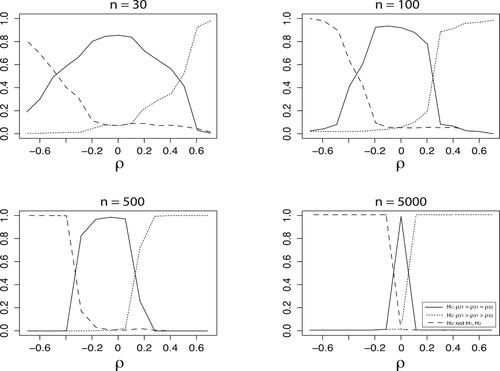
The plots show consistent behavior of the posterior probabilities for the hypotheses: as the sample size becomes very large the posterior probability of the true hypothesis goes to 1 and the posterior probabilities of the incorrect hypotheses goes to zero. Furthermore it can be seen that for small data sets with n = 30, relatively large effects (approximately $\rho =.5$) need to be observed before either $H_2$ or $H_3$ (depending on the sign of the effect) receives more evidence than the null hypothesis. This implies that a null hypothesis with a uniform prior is better able predict the data than the alternative hypotheses in the case of moderate effects and small samples. As the sample size grows very small and zero effects can best be explained by the null hypothesis, and larger effects can best be explained by the alternative hypotheses, depending on the direction.

For other types of hypothesis tests the rate of evidence increases in a similar fashion as the sample size grows. We refer the interested reader to the increasing literature that further explores the accumulation of the evidence in the data for a true hypothesis with equality, order, or interval constraints as the sample size grows (e.g. [8,14,43,46]).

6. Empirical applications from social science research (revisted)

6.1. Associations between life, leisure and relationship satisfaction

We now return to our empirical example and evaluate the informative hypotheses that we developed at the beginning of this contribution. Table 4 reports for each set of hypotheses the posterior probabilities that each hypothesis is true after observing the data when assuming equal prior probabilities for the hypotheses.

Table 4. Posterior probabilities for the competing hypotheses from Examples 1 and 2.

Application 1: Life, leisure,and relationship satisfaction
Hypothesis test 1	Posterior probabilities
$H_{1a}$: ${\rho }_{g1y2y1}>{\rho }_{g1y3y1}>{\rho }_{g1y3y2}$	0.0020
$H_{1b}$:${\rho }_{g1y3y1}>{\rho }_{g1y2y1}>{\rho }_{g1y3y2}$	0.0085
$H_{1c}$:${\rho }_{g1y3y1}={\rho }_{g1y2y1}={\rho }_{g1y3y2}$	0.9879
$H_{1d}$: neither $H_{1a}$, $H_{1b}$, nor $H_{1c}$	0.0016
Hypothesis test 2
$H_{2a}$: ${\rho }_{g2y2y1}>{\rho }_{g2y3y1}>{\rho }_{g2y3y2}$	0.0001
$H_{2b}$: ${\rho }_{g2y3y1}>{\rho }_{g2y2y1}>{\rho }_{g2y3y2}$	0.2955
$H_{2c}$: ${\rho }_{g2y3y1}={\rho }_{g2y2y1}={\rho }_{g2y3y2}$	0.2104
$H_{2d}$: neither $H_{2a}$, $H_{2b}$, nor $H_{2c}$	0.4940
Hypothesis test 3
$H_{3a}$: ${\rho }_{g1y2y1}>{\rho }_{g2y2y1}$	0.1588
$H_{3b}$: ${\rho }_{g1y2y1}={\rho }_{g2y2y1}$	0.8278
$H_{3c}$: ${\rho }_{g1y2y1}<{\rho }_{g2y2y1}$	0.0135
Hypothesis test 4
$H_{4a}$: ${\rho }_{g1y3y1}>{\rho }_{g2y3y1}$	0.0809
$H_{4b}$: ${\rho }_{g1y3y1}={\rho }_{g2y3y1}$	0.9017
$H_{4c}$: ${\rho }_{g1y3y1}<{\rho }_{g2y3y1}$	0.0174
Application 2: Support for justice principles
Hypothesis test 5
$H_{5a}$: ${\rho }_{g1y2y1}>{\rho }_{g2y2y1}>{\rho }_{g3y2y1}>{\rho }_{g4y2y1}$	0.0044
$H_{5b}$: ${\rho }_{g1y2y1}={\rho }_{g2y2y1}={\rho }_{g3y2y1}={\rho }_{g4y2y1}$	0.0000
$H_{5c}$: ${\rho }_{g1y2y1}={\rho }_{g2y2y1}>{\rho }_{g3y2y1}={\rho }_{g4y2y1}$	0.9899
$H_{5d}$: neither $H_{5a}$, $H_{5b}$, nor $H_{5c}$	0.0057

Based on these results we can conclude that for men there is overwhelming evidence of equal partial associations between life satisfaction, leisure satisfaction, and relationship satisfaction, controlling for differences in mood at survey and self-reported health (99%). For women on the other hand the evidence is inconclusive as the complement hypothesis, which receives most support, still only receives a posterior probability of approximately 49% after observing the data, and the ordered partial correlations hypothesis $H_{2b}$ and the equal partial correlations hypothesis $H_{2c}$ receive a posterior probability of 30% and 21%, respectively. More data need to be collected in order to draw more decisive conclusions about which hypothesis is true for the female population.

Next, we consider the hypotheses that expect either ordered or equal conditional (i.e. with gender as a moderator) partial associations between the satisfaction variables. Here, we see that there is strong evidence for the hypotheses that life satisfaction and each type of domain-specific satisfaction relate equally strong to each other for men and women (83%, and 90% respectively). In summary, the analysis portrays a picture of a large degree of equality of association between satisfaction indicators while holding constant for other variables, and little evidence for the expected ordering of partial associations among the variables considered.

6.2. Association between egalitarian justice beliefs across countries

Table 4 also reports the findings for the test of the informative hypotheses on the partial correlations between justice principles. Here, the findings indicate very strong evidence for Hypothesis $H_{5c}$. This equality and order-restricted hypothesis assumed that within the post-communist country cluster and within the Western European country cluster the partial correlation between support for both justice principles would be equal, but between country clusters the size of the partial correlation would be different, with an expected larger partial association in the post-communist group of countries.

7. Discussion

This paper presented a flexible framework for testing statistical hypotheses on most commonly observed measure of association in social research. By developing powerful, flexible and user-friendly Bayesian methods for testing informative hypotheses about partial correlations, we underscore the importance and appropriateness of the partial correlation coefficient as a tool for testing hypotheses about associations between variables of various measurement levels when applying regression analysis would actually not be appropriate from a research design or substantive perspective. The methodology has the following useful properties.

• A broad class of hypotheses can be tested with competing equality and/or order constraints on the measures of association (Table 1).

• Multiple (more than two) hypothese can be tested simultaneously in a straightforward manner.

• Constrained hypotheses can be formulated on tetrachoric correlations, polychoric correlations, biserial correlations, polyserial correlations, and product-moment correlations (Table 2). These measures of association can be corrected for certain covariates to avoid spurious relations.

• A simple answer is provided to the research question which hypothesis receives most evidence from the data and how much, using Bayes factors and posterior probabilities.

• The proposed test is consistent which implies that the posterior probability of the true hypothesis goes to one as the sample size goes to infinity.

• The software package BCT allows social science researchers to easily apply the methodology in real-life examples. The methodology for normally distributed dependent variables is also implemented in the R package BFpack [51,52], which also contains applications of equality/order constraints testing on correlations between continuous outcome variables. The extension to nonnormal data is planned for the near future.

The proposed methodology relies on the generalized multivariate probit model for continuous and ordinal outcome variables. This model is very well researched in the Bayesian literature (e.g. Albert and Chib [1], Chib and Greenberg [11], Chen and Dey [10], Barnard et al. [4]; Fox [17], Boscardin et al. [9]), and implemented in professional software packages such as Mplus [3] or Stata [63]. In the case of severe violations of the distributional assumptions (i.e. normality for continuous outcome variables and a normal latent variable for ordinal outcome variables), however, the estimated unconstrained posterior of the measures of association may not be accurate. To get a better understanding of the robustness of the method, a thorough numerical simulation study on this model would be useful. Potentially the method can also become more robust to violations of normality or the assumed probit model by adopting the rank likelihood approach of [20]. This will be an interesting future extension yielding a more accurate Bayes factor for testing measures of association in the case of severe model violations. Finally to further enhance the computation of Bayes factors for order hypotheses the use of bridge sampling techniques may prove fruitful when the number of order constraints is very large [60].

The proposed methodology was designed as a confirmatory criterion for testing multiple hypotheses with competing equality and/or order constraints on the measures of association of interest. The confirmatory aspect justifies the default use of equal prior probabilities of the hypotheses that are formulated. The method can also be used for exploratory testing of all possible hypotheses with combinations of equality and order constraints. In this case a correction for multiple testing is necessary because the number of hypotheses can become quite extensive. In a Bayesian framework such a correction can be incorporated through the prior probabilities of the hypotheses. Scott and Berger [61] showed how this can be done when exploratory testing many precise hypotheses. How this can be done when exploratory testing all possible equality and order hypotheses is still an open problem worthy of further research.

Finally the proposed Bayes factor test is based on uniform priors on the measures of association under the hypotheses of interest. This choice does not allow users to manually specify priors based on external prior beliefs about the measures of association. Although this may be viewed as a limitation, from a default ‘noninformative’ Bayesian perspective, the class of uniform priors seems the only justifiable choice because uniform priors imply that all possible values of the association in a correlation matrix measures are equally likely before observing the data. Furthermore, the proposed methodology is quite flexible as it allows researchers to formulate very specific hypotheses with equality and order constraints on the measures of association (Table 1). In fact by formulating hypotheses with very specific sets of constraints, very informative priors are implicitly specified. For example, when considering a hypothesis with equal correlations, $H_1:{\rho }_{12}={\rho }_{13}={\rho }_{23}$, the underlying prior is only positive (and constant) where all correlations are exactly equal. Similarly, the precise hypothesis $H_0:\rho =0$ corresponds to an extremely informative prior which places all its mass where ρ equals 0. Thus instead of allowing users to incorporate external information by directly specifying informative priors under the hypotheses, the methodology allows users to formulate very specific hypotheses which indirectly correspond to very informative priors. In our experience translating prior beliefs to constrained hypotheses is generally easier (and less controversial) than translating prior beliefs to informative priors on the parameters themselves. In certain applications however it may be preferred to use informative priors. This may be an interesting direction for future work. The current methodology was specifically developed for testing competing scientific expectations on measures of association in a default Bayesian manner.

Acknowledgments

The authors wish to thank Andrew Tomarken for helping with testing and debugging the ‘BCT’ software program, and Eric-Jan Wagenmakers and an anonymous reviewer for constructive feedback on an earlier version of the manuscript.

Disclosure statement

No potential conflict of interest was reported by the author(s).

Additional information

Funding

The first author was supported by a Veni Grant (016.145.205) provided by The Netherlands Organization for Scientific Research (NWO).

Notes

1 Consequently, the Bayes factor of an inequality constrained hypothesis against the unconstrained hypothesis can maximally be equal to the reciprocal of the prior probability that the constraints hold [47], and thus the nested test would not be consistent.

2 The uniform candidate prior, $\pi \left({\mathbf{\Sigma }}_g\right)\propto 1$, is equivalent to a joint uniform prior on ${\mathbf{C}}_g$ because the Jacobian of the transformation, ${\mathbf{\Sigma }}_g\to ({\mathit{\sigma }}_g,{\mathbf{C}}_g)$, does not depend on ${\mathbf{C}}_g$.

3 The integrated likelihood is given by Johnson and Kotz [26]: $f\left(r|\rho \right)=\frac{(1-{\rho }^2{)}^{(n-1)/2}(1-r^2{)}^{(n-4)/2}}{\pi (n-3)!}\frac{{\mathrm{d}}^{n-2}}{\mathrm{d}(\rho r{)}^{n-2}}\left\{\frac{{\cos }^{-1}(-\rho r)}{\sqrt{1-(\rho r{)}^2}}\right\}$.

4 The Fortran code for the sampler can be found on github.com/jomulder/BCT.

Appendices

Appendix 1.

The generalized multivariate probit model

This model is well-established in the Bayesian literature (e.g. [1,3,4,9–11,15,17,30,31,35,56]). We consider G independent populations. The P-dimension vector of dependent variables of subject i in population g will be denoted by ${\mathbf{y}}_{ig}^{\prime }=({\mathbf{v}}_{ig}^{\prime },{\mathbf{u}}_{ig}^{\prime })$, of which the first $P_1$ elements, ${\mathbf{v}}_{ig}^{\prime }=(v_{ig1},\dots ,v_{ig{P}_1})$, are continuous normally distributed variables and the remaining $P_2=P-P_1$ elements, ${\mathbf{u}}_{ig}^{\prime }=(u_{ig1},\dots ,u_{ig{P}_2})$, are measured on an ordinal scale, for $i=1,\dots ,n_g$, and $g=1,\dots ,G$. Furthermore, we assume that the pth ordinal variable can assume the categories $1,\dots ,K_p$, for $p=1,\dots ,P_2$.

As is common in a Bayesian multivariate probit modeling, a multivariate normal latent variable, denoted by ${\mathbf{z}}_{ig}$, is used for each ordinal vector ${\mathbf{u}}_{ig}$. This implies that the p ordinal variable of subject i in population g falls in category k, i.e. $u_{igp}=k,\text{if}{z}_{igp}\in ({\gamma }_{gp(k-1)},{\gamma }_{gpk}],$ for $k=1,\dots ,K_p$, where ${\gamma }_{gpk}$ is the upper cut-point of the kth category of the pth ordinal variable in the gth population. To ensure identification of the model it is necessary to set ${\gamma }_{gp0}=-\mathrm{\infty }$, ${\gamma }_{gp1}=0$, and ${\gamma }_{gp{K}_p}=\mathrm{\infty }$, for $g=1,\dots ,G$ and $p=1,\dots ,P_2$, and to fix the error variances of the latent variables to 1 as is common in multivariate probit modeling [11].

The mean structure of each dependent variable is assumed to be a linear combination of Q external covariates ${\mathbf{x}}_{ig}$. Subsequently, the generalized multivariate probit model can be defined by (A1) $\begin{array}{rl}\left[\begin{array}{c}{\mathbf{v}}_{ig}\\ {\mathbf{z}}_{ig}\end{array}\right]& \sim N({\mathbf{B}}_g{\mathbf{x}}_{ig},{\mathbf{\Sigma }}_g),\text{where}\end{array}$(A1) (A2) $\begin{array}{rl}{\mathbf{\Sigma }}_g& =\text{diag}({\mathit{\sigma }}_g^{\prime },{\mathbf{1}}_{P_2}^{\prime }){\mathbf{C}}_g\text{diag}({\mathit{\sigma }}_g^{\prime },{\mathbf{1}}_{P_2}^{\prime }),\end{array}$(A2) where ${\mathbf{1}}_{P_2}^{\prime }$ is a vector of length $P_2$ of ones. Notice here that the correlation matrices ${\mathbf{C}}_g$ and standard deviations ${\mathit{\sigma }}_g$ are separately modeled as in [4]. In this model ${\mathbf{B}}_g$ is a $P\times Q$ matrix with regression coefficients of the gth population where element $(p,q)$ reflects the effect of the qth covariate on the pth dependent variable, for $q=1,\dots ,Q$ and $p=1,\dots ,P$, the $P_1$ error standard deviations of ${\mathbf{v}}_{ig}$ in population g are contained in ${\mathit{\sigma }}_g$, and ${\mathbf{C}}_g$ denotes the $P\times P$ correlation matrix of population g. Note that the $(p_1,p_2)$th element of ${\mathbf{C}}_g$ denotes the linear association of the $p_1$th and $p_2$th dependent variable in population g while controlling for the covariates in ${\mathbf{x}}_{ig}$. Thus, if a model is specified with two dependent variables and several covariates, and we would be interested in testing ${\rho }_{12}=0$, we are essentially testing the partial correlation between the two dependent variables while controlling for the covariates that are included in ${\mathbf{x}}_{ig}$. This way no distributional assumptions are made about the covariates because they are included as independent variables in the regression model. For example one can include covariates that are only 0 or 1 to correct for a categorical variable. If Q = 1 and $x_{ig}=1$, no covariates are incorporated in the model, which implies that the elements in ${\mathbf{C}}_g$ are bivariate correlations.

Appendix 2.

Derivation of the priors

Implied prior by Wetzels and Wagenmakers [68]

Assume we are interested in the correlation ρ between Y and X having a bivariate normal distribution, $\left[\begin{array}{c}Y\\ X\end{array}\right]\sim N\left(\left[\begin{array}{c}{\mu }_Y\\ {\mu }_X\end{array}\right],\left[\begin{array}{cc}{\sigma }_Y^2& \rho {\sigma }_Y{\sigma }_X\\ \rho {\sigma }_Y{\sigma }_X& {\sigma }_X^2\end{array}\right]\right),$ where ρ is the correlation between Y and X. We assume that the variable X is normalized, i.e. ${\mu }_X=0$ and ${\sigma }_X^2=1$. The bivariate normal model correspond with the following conditional formulation, (A3) $Y|X\sim N({\mu }_Y+\rho {\sigma }_{Y}X,{\sigma }_Y^2(1-{\rho }^2\left)\right).$(A3) Now we consider an alternative parameterization using a linear regression model (A4) $Y|X\sim N({\text{β}}_0+{\text{β}}_{1}X,{\sigma }_{ϵ}^2)$(A4) where ${\sigma }_{ϵ}^2$ is the error variance in the regression model. When linking these two parameterizations, this implies ${\text{β}}_1=\rho {\sigma }_Y=\rho (1-{\rho }^2{)}^{-1}{\sigma }_{ϵ}\iff \rho =\frac{{\text{β}}_1}{\sqrt{{\text{β}}_1^2+{\sigma }_{ϵ}^2}}.$ Hence, testing $H_0:\rho =0$ against $H_1:\rho \ne 0$ in (A3(A3) $Y|X\sim N({\mu }_Y+\rho {\sigma }_{Y}X,{\sigma }_Y^2(1-{\rho }^2\left)\right).$(A3) ) is equivalent to testing $H_0:{\text{β}}_1=0$ against $H_1:{\text{β}}_1\ne 0$ in (A4(A4) $Y|X\sim N({\text{β}}_0+{\text{β}}_{1}X,{\sigma }_{ϵ}^2)$(A4) ).

Wetzels and Wagenmakers [68] considered a g prior for ${\text{β}}_1$ with an inverse gamma with a shape parameter of $\frac{1}{2}$ and a scale parameter of $\frac{n}{2}$, which is equivalent to a Student t prior with zero location, a scale of ${\sigma }_{ϵ}^2$, and 1 degree of freedom (i.e. a Cauchy prior): $\begin{array}{rl}{\pi }_1\left({\text{β}}_1|{\sigma }_{ϵ}^2\right)& =\int N({\text{β}}_1;0,g{\sigma }_{ϵ}^2({\mathbf{x}}^{\prime }\mathbf{x}{)}^{-1})IG\left(g;\frac{1}{2},\frac{n}{2}\right)\mathrm{d}g\\ & =t({\text{β}}_1;0,{\sigma }_{ϵ}^2,1)\\ & \propto (1+{\text{β}}_1^2/{\sigma }_{ϵ}^2{)}^{-1},\end{array}$ where we set ${\mathbf{x}}^{\prime }\mathbf{x}=n$. When noting that the Jacobian equals $\frac{\mathrm{d}{\text{β}}_1}{\mathrm{d}\rho }={\sigma }_{ϵ}\left({\rho }^2\right(1-{\rho }^2{)}^{-3/2}+(1-{\rho }^2{)}^{-1/2})$, the prior for ρ can be obtained by applying standard calculus, i.e. $\begin{array}{rl}{\pi }_1\left(\rho |{\sigma }_{ϵ}^2\right)& ={\pi }_1({\text{β}}_1=\rho (1-{\rho }^2{)}^{-1}{\sigma }_{ϵ}|{\sigma }_{ϵ}^2)\frac{\mathrm{d}{\text{β}}_1}{\mathrm{d}\rho }\\ & \propto {\left(1+{\rho }^2(1-{\rho }^2{)}^{-1}\right)}^{-1}\left({\rho }^2\right(1-{\rho }^2{)}^{-3/2}+(1-{\rho }^2{)}^{-1/2})\\ & =(1-{\rho }^2{)}^{-1/2}\\ & \propto beta(\frac{1}{2},\frac{1}{2})\mathrm{i}\mathrm{n}\mathrm{t}\mathrm{h}\mathrm{e}\mathrm{i}\mathrm{n}\mathrm{t}\mathrm{e}\mathrm{r}\mathrm{v}\mathrm{a}\mathrm{l}(-1,1).\end{array}$ Similarly, it can be shown that a uniform prior for ρ in the interval $(-1,1)$ would correspond to conditional prior for ${\text{β}}_1$ given ${\sigma }_{ϵ}^2$ with a Student t distribution with location, scale, and degrees of freedom equal to 0, ${\sigma }_{ϵ}^2/2$, and 2, respectively.

Marginally uniform prior approach

As shown by Barnard et al. [4] an inverse Wishart prior with identity scale matrix $\mathbf{P}$ and P degrees of freedom for a covariance matrix implies a marginal prior for a correlation matrix $\mathbf{C}$ having a density $\pi \left(\mathbf{C}\right)\propto |\mathbf{C}{|}^{\frac{(P-1{)}^2}{2}-1}\prod _{p=1}^P|{\mathbf{C}}_{pp}{|}^{-P/2},$ where ${\mathbf{C}}_{pp}$ is the pth principle submatrix of $\mathbf{C}$. Now consider a hypothesis where all correlations are assumed to be equal (which implies a compound symmetry correlation structure), $H_0:{\rho }_{21}=\dots ={\rho }_{P,P-1}$. The determinants are then a function of the common correlation ρ and given by $|\mathbf{C}|=\left(\right(P-1)\rho +1)(1-\rho {)}^{P-1}$ and $|{\mathbf{C}}_{pp}|=\left(\right(P-2)\rho +1)(1-\rho {)}^{P-2}$. Consequently, the implied prior for ρ under $H_0$ is given by ${\pi }_0\left(\rho \right)\propto \left(\rho \right(P-1)+1{)}^{\frac{(P-1{)}^2}{2}-1}(1-\rho {)}^{-\frac{P^2-P-1}{2}}\left(\rho \right(P-2)+1{)}^{-\frac{P^2}{2}},$ which, for P = 3, equals ${\pi }_0\left(\rho \right)\propto (2\rho +1)(1-\rho {)}^{-5/2}(\rho +1{)}^{-9/2}.$

Appendix 3.

Proof of Lemma 1

The proof is based on the results of [28,43,47,49,55,67]. The constrained hypothesis $H_t$ is given by $H_t:{\mathbf{R}}^E\mathit{\rho }={\mathbf{r}}^E,{\mathbf{R}}^I\mathit{\rho }>{\mathbf{r}}^I$, where $\left[{\mathbf{R}}^E|{\mathbf{r}}^E\right]$ is a $q^E\times (Q+1)$ augmented matrix representing the equality constraints on $\mathit{\theta }$, with $q^E\le Q$, and $\left[{\mathbf{R}}^I|{\mathbf{r}}^I\right]$ is a $q^I\times (Q+1)$ augmented matrix representing the inequality constraints on $\mathit{\rho }$.

Under $H_t$ there are $q^E$ equality constraints active on $\mathit{\rho }$, which will be denoted by ${\mathit{\rho }}_t^I={\mathbf{R}}_t^I\mathit{\rho }$. Therefore there are $Q-q^E$ free parameters under $H_t$ (excluding the nuisance parameters), which we shall denote by ${\mathit{\rho }}_t^I$. Without loss of generality we can permute the elements of $\mathit{\rho }$, such that we can write $\left[\begin{array}{c}{\mathit{\rho }}_t^E\\ {\mathit{\rho }}_t^I\end{array}\right]=\left[\begin{array}{c}{\mathbf{R}}_t^E\\ \mathbf{0}{\mathbf{I}}_{Q-q^E}\end{array}\right]\mathit{\rho }.$ Consequently, the constrained hypothesis can equivalently be written as $H_t:{\mathit{\rho }}_t^E={\mathbf{r}}_t^E,{\tilde{\mathbf{R}}}_t^I{\mathit{\rho }}_t^I>{\mathbf{r}}_t^I$, where ${\tilde{\mathbf{R}}}_t^I$ consists of the last $Q-q^E$ columns of ${\mathbf{R}}_t^I$.

The prior under $H_t$ is a truncation of the unconstrained prior under $H_u$ in the constrained space of $H_t$, i.e. $\begin{array}{rl}{\pi }_t\left({\mathit{\rho }}_t^I\right)& =c_t^{-1}{\pi }_u({\mathit{\rho }}_t^E={\mathbf{r}}_t^E,{\mathit{\rho }}_t^I)I({\tilde{\mathbf{R}}}_t^I{\mathit{\rho }}_t^I>{\mathbf{r}}_t^I),\mathrm{w}\mathrm{h}\mathrm{e}\mathrm{r}\mathrm{e}\\ c_t& =\mathrm{P}\mathrm{r}({\tilde{\mathbf{R}}}_t^I{\mathit{\rho }}_t^I>{\mathbf{r}}_t^I|{\mathit{\rho }}_t^E={\mathbf{r}}_t^E,H_u){\pi }_u({\mathit{\rho }}_t^E={\mathbf{r}}_t^E).\end{array}$ Furthermore, the nuisance parameters have equal priors under both the constrained and unconstrained hypothesis, i.e. ${\pi }_t\left(\mathit{\varphi }\right)={\pi }_u\left(\mathit{\varphi }\right)$, and the likelihood of the data under $H_t$ is a truncation of the unconstrained likelihood, i.e. $p_t(\mathbf{Y}|\mathbf{X},{\mathit{\rho }}_t^I,\mathit{\varphi })=p_u(\mathbf{Y}|\mathbf{X},{\mathit{\rho }}_t^E={\mathbf{r}}_t^E,{\mathit{\rho }}_t^I,\mathit{\varphi })I({\tilde{\mathbf{R}}}_t^I{\mathit{\rho }}_t^I>{\mathbf{r}}_t^I),$ where $\mathbf{Y}$ contains all outcome variables and $\mathbf{X}$ contains all covariates. The Bayes factor can then be written as $\begin{array}{rl}{B}_{tu}& =\frac{{\iint }_{{\tilde{\mathbf{R}}}_t^I{\mathit{\rho }}_t^I>{\mathbf{r}}_t^I}{\pi }_t\left({\mathit{\rho }}_t^I\right){\pi }_t\left(\mathit{\varphi }\right)p_t(\mathbf{Y}|\mathbf{X},{\mathit{\rho }}_t^I,\mathit{\varphi })\mathrm{d}{\mathit{\rho }}_t^I\mathrm{d}\mathit{\varphi }}{\iiint {\pi }_u({\mathit{\rho }}_t^E,{\mathit{\rho }}_t^I){\pi }_u\left(\mathit{\varphi }\right)p_u(\mathbf{Y}|\mathbf{X},{\mathit{\rho }}_t^E,{\mathit{\rho }}_t^I,\mathit{\varphi })\mathrm{d}{\mathit{\rho }}_t^E\mathrm{d}{\mathit{\rho }}_t^I\mathrm{d}{\mathit{\rho }}_t^I\mathrm{d}\mathit{\varphi }}\\ & =\frac{{\iint }_{{\tilde{\mathbf{R}}}_t^I{\mathit{\rho }}_t^I>{\mathbf{r}}_t^I}{c}_t^{-1}{\pi }_u({\mathit{\rho }}_t^E={\mathbf{r}}_t^E,{\mathit{\rho }}_t^I){\pi }_u\left(\mathit{\varphi }\right)p_u(\mathbf{Y}|\mathbf{X},{\mathit{\rho }}_t^E={\mathbf{r}}_t^E,{\mathit{\rho }}_t^I,\mathit{\varphi })\mathrm{d}{\mathit{\rho }}_t^I\mathrm{d}\mathit{\varphi }}{\iiint {\pi }_u({\mathit{\rho }}_t^E,{\mathit{\rho }}_t^I){\pi }_u\left(\mathit{\varphi }\right)p_u(\mathbf{Y}|\mathbf{X},{\mathit{\rho }}_t^E,{\mathit{\rho }}_t^I,\mathit{\varphi })\mathrm{d}{\mathit{\rho }}_t^E\mathrm{d}{\mathit{\rho }}_t^I\mathrm{d}{\mathit{\rho }}_t^I\mathrm{d}\mathit{\varphi }}\\ & =c_t^{-1}{\iint }_{{\tilde{\mathbf{R}}}_t^I{\mathit{\rho }}_t^I>{\mathbf{r}}_t^I}\frac{{\pi }_u({\mathit{\rho }}_t^E={\mathbf{r}}_t^E,{\mathit{\rho }}_t^I){\pi }_u\left(\mathit{\varphi }\right)p_u(\mathbf{Y}|\mathbf{X},{\mathit{\rho }}_t^E={\mathbf{r}}_t^E,{\mathit{\rho }}_t^I,\mathit{\varphi })}{\iiint {\pi }_u({\mathit{\rho }}_t^E,{\mathit{\rho }}_t^I){\pi }_u\left(\mathit{\varphi }\right)p_u(\mathbf{Y}|\mathbf{X},{\mathit{\rho }}_t^E,{\mathit{\rho }}_t^I,\mathit{\varphi })\mathrm{d}{\mathit{\rho }}_t^E\mathrm{d}{\mathit{\rho }}_t^I\mathrm{d}{\mathit{\rho }}_t^I\mathrm{d}\mathit{\varphi }}\mathrm{d}{\mathit{\rho }}_t^I\mathrm{d}\mathit{\varphi }\\ & =c_t^{-1}{\iint }_{{\tilde{\mathbf{R}}}_t^I{\mathit{\rho }}_t^I>{\mathbf{r}}_t^I}{\pi }_u({\mathit{\rho }}_t^E={\mathbf{r}}_t^E,{\mathit{\rho }}_t^I,\mathit{\varphi }|\mathbf{Y},\mathbf{X})\mathrm{d}{\mathit{\rho }}_t^I\mathrm{d}\mathit{\varphi }\\ & =\frac{\mathrm{P}\mathrm{r}({\tilde{\mathbf{R}}}_t^I{\mathit{\rho }}_t^I>{\mathbf{r}}_t^I|{\mathit{\rho }}_t^E={\mathbf{r}}_t^E,\mathbf{Y},\mathbf{X},H_u){\pi }_u({\mathit{\rho }}_t^E={\mathbf{r}}_t^E|\mathbf{Y},\mathbf{X})}{\mathrm{P}\mathrm{r}({\tilde{\mathbf{R}}}_t^I{\mathit{\rho }}_t^I>{\mathbf{r}}_t^I|{\mathit{\rho }}_t^E={\mathbf{r}}_t^E,H_u){\pi }_u({\mathit{\rho }}_t^E={\mathbf{r}}_t^E)},\end{array}$ which completes the proof.

Appendix 4.

Conditional distributions for the MCMC sampler

For $g=1,\dots ,G$, the group specific parameters are sampled in the posterior as follows.

1. Sample ${\mathbf{B}}_g|{\mathbf{V}}_g,{\mathbf{U}}_g,{\mathbf{Z}}_g,{\mathbf{X}}_g,{\mathit{\sigma }}_g,{\mathbf{C}}_g\sim N_{Q\times P}({\hat{\mathbf{B}}}_g,({\mathbf{X}}_g^{\prime }{\mathbf{X}}_g{)}^{-1},{\mathbf{\Sigma }}_g)$, where ${\hat{\mathbf{B}}}_g=({\mathbf{X}}_g^{\prime }{\mathbf{X}}_g{)}^{-1}{\mathbf{X}}_g^{\prime }{\mathbf{Y}}_g^{\ast }$, ${\mathbf{Y}}_g^{\ast }=\left[{\mathbf{V}}_g{\mathbf{Z}}_g\right]$, i.e. a stacked matrix of $({\mathbf{v}}_{ig}^{\prime },{\mathbf{z}}_{ig}^{\prime })$, for $i=1,\dots ,n_g$, and ${\mathbf{\Sigma }}_g=\mathrm{d}\mathrm{i}\mathrm{a}\mathrm{g}({\mathit{\sigma }}_g^{\prime },{\mathbf{1}}_{P_2}^{\prime }){\mathbf{C}}_g\mathrm{d}\mathrm{i}\mathrm{a}\mathrm{g}({\mathit{\sigma }}_g^{\prime },{\mathbf{1}}_{P_2}^{\prime })$;

2. Sample ${\mathbf{C}}_g$ given ${\mathbf{B}}_g$, ${\mathbf{V}}_g$, ${\mathbf{U}}_g$, ${\mathbf{Z}}_g$, ${\mathbf{X}}_g$, ${\mathit{\sigma }}_g$ using a parameter expansion of [34]. Let ${\mathbf{E}}_g={\mathbf{Y}}_g^{\ast }-{\mathbf{X}}_g{\mathbf{B}}_g$, and the normalization of the columns ${\tilde{\mathbf{E}}}_g={\mathbf{E}}_g{\mathbf{D}}_g$, where $\sum _{i=1}^{n_g}{\tilde{e}}_{gi}^2=1$. The positive definite scale is then given by ${\mathbf{S}}_g=\mathrm{d}\mathrm{i}\mathrm{a}\mathrm{g}(1/{\mathit{\sigma }}_g^{\prime },{\mathbf{1}}_{P_2}^{\prime }){\tilde{\mathbf{E}}}_g^{\prime }{\tilde{\mathbf{E}}}_g\mathrm{d}\mathrm{i}\mathrm{a}\mathrm{g}(1/{\mathit{\sigma }}_g^{\prime },{\mathbf{1}}_{P_2}^{\prime })$. Furthermore a uniform candidate prior is considered for the covariance matrix, i.e. $\pi \left({\mathbf{\Sigma }}_g\right)\propto 1$, such that the candidate covariance matrix can be drawn from an inverse Wishart distribution, $IW(n_g-P-1,{\mathbf{S}}_g)$, from which the candidate draw for ${\mathbf{C}}_g$ can be obtained which is always accepted because the target prior for the correlation matrix is the same².

3. The threshold parameter ${\gamma }_{gpk}$, for $p=P_1,\dots ,P$, and $k=2,\dots ,K_p-1$, is sampled from a uniform distribution with lowerbound being the largest $z_{gip}$ that falls in the category k−1, and upperbound being the smallest $z_{gip}$ that falls in the category k.

4. The population standard deviation ${\sigma }_p$, for $p=1,\dots ,P_1$, is sampled using a random walk centered around the previous draw (see also [34]).

5. The additional parameters due to the parameter extension of [35] are sampled using a random walk centered around the previous draw. The following scale group is chosen, $\begin{array}{rl}{\mathrm{\Gamma }}_{gp}& =\{h_{gp}>0:h_{gp}({\mathbf{z}}_{gp},{\mathbf{B}}_{\cdot p},{\gamma }_{gp2},\dots ,{\gamma }_{gp(K_p-1)})\\ & =(h_{gp}{\mathbf{z}}_{gp},h_{gp}{\mathbf{B}}_{\cdot p},h_{gp}{\gamma }_{gp2},\dots ,h_{gp}{\gamma }_{gp(K_p-1)})\},\end{array}$ for group g and dimension p, for $p=P_1,\dots ,P$. The unimodular Haar measure for ${\mathrm{\Gamma }}_{gp}$ is $L\left(d{h}_{gp}\right)=h_{gp}^{-1}d{h}_{gp}$. To sample $h_{gp}$ using the random walk, the kernel for $h_{gp}$ is of the form $h_{gp}^{n_g+Q+K_p-3}\exp (-a_{gp}{h}_{gp}^2-b_{gp}{h}_{gp})$.

The Fortran code for the MCMC algorithm can be found on github.com/jomulder/BCT.

Appendix 5.

Numerical computation of the Bayes factor

We discuss a general numerical method to compute the elements in (15(15) $B_{tu}=\frac{\text{Pr}({\tilde{\mathbf{R}}}_t^I{\mathit{\rho }}_t^I>{\mathbf{r}}_t^I|{\mathit{\rho }}_t^E={\mathbf{r}}_t^E,H_u,\mathbf{Y},\mathbf{X})}{\text{Pr}({\tilde{\mathbf{R}}}_t^I{\mathit{\rho }}_t^I>{\mathbf{r}}_t^I|{\mathit{\rho }}_t^E={\mathbf{r}}_t^E,H_u)}\times \frac{{\pi }_u({\mathit{\rho }}_t^E={\mathbf{r}}_t^E|\mathbf{Y},\mathbf{X})}{{\pi }_u({\mathit{\rho }}_t^E={\mathbf{r}}_t^E)},$(15) ) for a hypothesis $H_t$ with equality and/or inequality constraints on the measures of association in the generalized multivariate probit model in Section 3.1 using the uniform prior discussed in Section 4.2. The computation of the posterior parts in the numerators in (15(15) $B_{tu}=\frac{\text{Pr}({\tilde{\mathbf{R}}}_t^I{\mathit{\rho }}_t^I>{\mathbf{r}}_t^I|{\mathit{\rho }}_t^E={\mathbf{r}}_t^E,H_u,\mathbf{Y},\mathbf{X})}{\text{Pr}({\tilde{\mathbf{R}}}_t^I{\mathit{\rho }}_t^I>{\mathbf{r}}_t^I|{\mathit{\rho }}_t^E={\mathbf{r}}_t^E,H_u)}\times \frac{{\pi }_u({\mathit{\rho }}_t^E={\mathbf{r}}_t^E|\mathbf{Y},\mathbf{X})}{{\pi }_u({\mathit{\rho }}_t^E={\mathbf{r}}_t^E)},$(15) ) is discussed first, followed by the prior parts in the denominators.

A.1. Computation of the posterior probability and posterior density

To compute the posterior probability and the posterior density in the numerators in (15(15) $B_{tu}=\frac{\text{Pr}({\tilde{\mathbf{R}}}_t^I{\mathit{\rho }}_t^I>{\mathbf{r}}_t^I|{\mathit{\rho }}_t^E={\mathbf{r}}_t^E,H_u,\mathbf{Y},\mathbf{X})}{\text{Pr}({\tilde{\mathbf{R}}}_t^I{\mathit{\rho }}_t^I>{\mathbf{r}}_t^I|{\mathit{\rho }}_t^E={\mathbf{r}}_t^E,H_u)}\times \frac{{\pi }_u({\mathit{\rho }}_t^E={\mathbf{r}}_t^E|\mathbf{Y},\mathbf{X})}{{\pi }_u({\mathit{\rho }}_t^E={\mathbf{r}}_t^E)},$(15) ) under the unconstrained hypothesis, the unconstrained marginal posterior for $\mathit{\rho }$ needs to approximated. This is done using posterior draws of the parameters from the unconstrained generalized multivariate probit model (Section 3.1) using a MCMC sampler. To sample the group specific correlation matrices ${\mathbf{C}}_g$, the Metropolis–Hastings step of [34] is extended to the generalized multivariate probit model with both continuous and ordinal outcome variables. Furthermore, to ensure fast mixing of the threshold parameters, the parameter expansion method of [35] is extended to the generalized multivariate probit model with a scale group that is unique for each group and each dimension p, for $p=P_1,\dots ,P$. The parameter expansion of Liu and Sabatti's [35] has been shown to be superior to other sampling procedures [56]. Details about the conditional distributions are given in Appendix 3. The Fortran code of the MCMC algorithm can be found on Github/jomulder/BCT.

Next, a Fisher z-transformation is applied to the unconstrained posterior sample for $\mathit{\rho }$. Let ${\rho }_{p_1{p}_2}$ be the association between the $p_1$th and $p_2$th dependent variable. Then, ${\eta }_{p_1{p}_2}=\frac{1}{2}\log \left(\frac{1+{\rho }_{p_1{p}_2}}{1-{\rho }_{p_1{p}_2}}\right)$ is the corresponding Fisher transformed measure of association. The unconstrained posterior of the Fisher transformed parameter follows an approximate normal distribution. This can be seen as follows. First note that the posterior is proportional to the likelihood times the prior. In this paper, a flat (uniform) prior is used for the correlations, and thus, the posterior is essentially proportional to the likelihood. In the integrated likelihood (where the nuisance parameters are integrated out) the sample correlation r is known to have a similar role as the population correlation ρ³. Now because the Fisher transformed sample correlation given the population correlation is also known to be approximately normal, the Fisher transformed population correlation given the sample correlation (i.e. the integrated posterior) will also be approximately normal.

To illustrate the accuracy of the normal approximation, a sample of size n = 40 was generated from a generalized multivariate probit model with P = 3 dimensions where the first dependent variable was normally distributed, the second dependent variable was ordinal with two categories, and the third dependent variable was ordinal with four categories. The population variables were set to ${\mathit{\rho }}^{\prime }=({\rho }_{21},{\rho }_{31},{\rho }_{32})=(.25,.25,0)$. A posterior sample of 10,000 draws was obtained for $\mathit{\rho }$ and transformed to the respective Fisher transformed parameters $\mathit{\eta }=({\eta }_{21},{\eta }_{31},{\eta }_{32})$. The traceplots for the first 1,000 draws for four different latent z-scores belonging to observations in the four different categories of the third outcome variable together with the corresponding threshold parameters are plotted in Figure A1 (left panel), and the posterior draws of $({\eta }_{21},{\eta }_{31})$ are plotted in Figure A1 (right panel) together with a contour plot of the bivariate density and the density estimates of the univariate posteriors. Normal approximations are also displayed (dashed lines). As can be seen the normal approximation is very accurate. For other settings (e.g. different dimensions or measurement levels of the outcome variables), the plots looked very similar. For larger samples, the normal approximations are even better. Consequently note that the posterior of the transformed measures of association under an inequality constrained hypothesis would follow an approximately normal distribution truncated in the inequality constrained subspace.

Figure A1. Left panel: Trace plot of latent $z_{31}$ observed in category 1 of the 3th (ordinal) outcome variable (blue line), $z_{32}$ observed in category 2 (orange line), $z_{33}$ observed in category 3 (green line), and $z_{34}$ observed in category 4 (purple line), as well as the corresponding threshold parameters ${\gamma }_{31}$, ${\gamma }_{32}$, and ${\gamma }_{34}$ for the 3th outcome variable. Right panel: Scatter plot of posterior draws of $({\eta }_{21},{\eta }_{31})$ (red dots) with additional contour plot and univariate density plots (solid lines) and normal approximations (dashed lines).

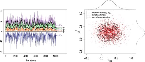
Thus, we can write $\pi \left(\mathit{\eta }|\mathbf{Y}\right)\approx N({\mathit{\mu }}_{\mathit{\eta }},{\mathbf{\Sigma }}_{\mathit{\eta }})$, where the posterior mean ${\mathit{\mu }}_{\mathit{\eta }}$ and covariance matrix ${\mathbf{\Sigma }}_{\mathit{\eta }}$ can be estimated from the posterior sample. Subsequently, the linear transformation $\mathit{\xi }=\mathbf{T}\mathit{\eta }$ is used, with $\mathbf{T}=\left[{\mathbf{R}}_t^{E^{\prime }}{\mathbf{R}}_t^{\prime }\right]$ as in Lemma 1. Approximately normality also holds for $\mathit{\xi }$, with $\pi \left(\mathit{\xi }|\mathbf{Y}\right)\approx N(\mathbf{T}{\mathit{\mu }}_{\mathit{\eta }},\mathbf{T}{\mathbf{\Sigma }}_{\mathit{\eta }}{\mathbf{T}}^{\prime })$. Therefore, the posterior density can be estimated by plugging in ${\mathit{\xi }}^E={\mathbf{r}}_t^E$ in the multivariate normal density $\pi \left({\mathit{\xi }}^E|\mathbf{Y}\right)\approx N({\mathbf{R}}_t^E{\mathit{\mu }}_{\mathit{\eta }},{\mathbf{R}}_t^E{\mathbf{\Sigma }}_{\mathit{\eta }}{\mathbf{R}}_t^{E^{\prime }})$. The conditional posterior probability can also be efficiently computed using the normal approximation. First the inequality constraints are rewritten via a linear transformation, e.g. $Pr({\eta }_{21}<{\eta }_{31}<{\eta }_{32})=Pr({\zeta }_1>0,{\zeta }_2>0)=Pr({\zeta }_1>0|{\zeta }_2>0)\times Pr({\zeta }_2>0)$ where $({\zeta }_1,{\zeta }_2)=({\eta }_{31}-{\eta }_{21},{\eta }_{32}-{\eta }_{31})$ [44]. The conditional probabilities can then be estimated efficiently from MCMC output [19,41].

A.2. Computation of the prior probability and prior density

Similar as the posterior components, the conditional prior probability and prior density in (15(15) $B_{tu}=\frac{\text{Pr}({\tilde{\mathbf{R}}}_t^I{\mathit{\rho }}_t^I>{\mathbf{r}}_t^I|{\mathit{\rho }}_t^E={\mathbf{r}}_t^E,H_u,\mathbf{Y},\mathbf{X})}{\text{Pr}({\tilde{\mathbf{R}}}_t^I{\mathit{\rho }}_t^I>{\mathbf{r}}_t^I|{\mathit{\rho }}_t^E={\mathbf{r}}_t^E,H_u)}\times \frac{{\pi }_u({\mathit{\rho }}_t^E={\mathbf{r}}_t^E|\mathbf{Y},\mathbf{X})}{{\pi }_u({\mathit{\rho }}_t^E={\mathbf{r}}_t^E)},$(15) ), are computed by first approximating the unconstrained uniform prior using a prior sample. This can be done using the algorithm of [25].⁴ To avoid the Borel-Kolmogorov paradox in the case of equality constraints [67], the Fisher transformation is also applied to the prior draws of the ρ's, resulting in prior draws for the corresponding η's. Substantially similarly as for the posterior, a linear transformation is applied to the prior draws for $\mathit{\xi }$, i.e. $\mathit{\xi }=\mathbf{T}\mathit{\eta }$. Unlike the posterior, the prior of $\mathit{\xi }$ is not approximately normal.

To estimate the prior density of $\mathit{\xi }$ at ${\tilde{\mathbf{r}}}_t^E$, (i.e. the Fisher transformed values of ${\mathbf{r}}_t^E$), we use the fact that $Pr(|{\xi }_1-{\tilde{r}}_1^E|<\frac{\delta }{2},\dots ,|{\xi }_{q^E}-{\tilde{r}}_{q^E}^E|<\frac{\delta }{2}|H_u)\approx {\delta }^{q^E}\times {\pi }_u({\mathit{\xi }}^E={\tilde{\mathbf{r}}}^E)$ for sufficiently small δ. Because a large prior sample can efficiently be obtained without needing MCMC, estimating the above probability as the proportion of draws satisfying the constraints is quite efficient. Thus, the prior density will be estimated as ${\hat{\pi }}_u({\mathit{\xi }}^E={\tilde{\mathbf{r}}}^E)={\delta }^{-q^E}{S}^{-1}\sum _{s=1}^{S}I(|{\xi }_1^{\left(s\right)}-{\tilde{r}}_1^E|<\frac{\delta }{2},\dots ,|{\xi }_{q^E}^{\left(s\right)}-{\tilde{r}}_{q^E}^E|<\frac{\delta }{2}),$ for sufficiently large S and a some small value for $\delta >0$.

To compute the conditional prior probability, we approximate the prior conditional of ${\mathit{\xi }}^I$ given ${\mathit{\xi }}^E={\tilde{\mathbf{r}}}^E$ with a normal distribution where the mean and covariance matrix are estimated as the arithmetic mean and the least squares estimate based on the prior draws that satisfy ${\mathit{\xi }}^E\approx {\tilde{\mathbf{r}}}^E$, respectively. The same approximation is used as for the equality constraints, i.e. $|{\xi }_q^{\left(s\right)}-{\tilde{r}}_q^E|<\frac{\delta }{2}$, for $q=1,\dots ,q^E$, where ${\xi }_q^{\left(s\right)}$ is the sth draw of ${\xi }_q$. A normal approximation is justified for the computation of the conditional prior probability because this probability is not very sensitive to the exact distributional form. For example, the probability that a parameter is larger than 0 is identical for a uniform distribution in $(-1,1)$ as for a standard normal distribution or for any other symmetrical distribution around zero. Note that this is not the case for the prior density at 0 which is why a normal approximation was not used for estimating the prior density. Based on the normal approximation, which can be summarized as ${\pi }_u({\mathit{\xi }}^E\approx {\mathbf{r}}^E)\approx N({\mathit{\mu }}_{\mathit{\xi }0},{\mathbf{\Sigma }}_{\mathit{\xi }0})$, the same procedure can be used for estimating the conditional prior probability of ${\mathbf{R}}_t^I{\mathbf{T}}^{-1}[{\mathbf{r}}^{E^{\prime }},{\mathit{\xi }}^{I^{\prime }}{]}^{\prime }>{\mathbf{r}}_t^I$, as was used for the conditional posterior probability.

Appendix 6.

User manual for BCT

The software program BCT (Bayesian Correlation Testing) can be downloaded from www.jorismulder.com. The folder consist of six text files, i.e. BCT_input.txt, BCT_output.txt, BCT_output_relComp.txt, BCT_output_relFit.txt, BCT_estimates.txt, and data.txt, and an executable file BCT.exe. BCT can be run by double clicking ‘BCT.exe’. This manual describes how to specify the input and data files and how to read the output file.

Parameterization

The hypotheses are tested under the generalized multivariate probit model which assumes multivariate normal distribution for the continuous dependent variables and multivariate probit distribution (with a multivariate normal distribution for the latent variables) for the ordinal dependent variables. Multiple populations can be considered having population specific intercepts, regression coefficients, variances and measures of associations.

Input file

This input file ‘BCT_input.txt’ has the following layout.

Under ‘Input 1’ the properties of the model have to specified that is used for analyzing the data. In the above example the model has 3 dependent variables (#DV=3), 2 covariates (#covs=2), an intercept should be included in the model (#intercept=1), is used for modeling one population (#population=1), and the total sample size is 50 (#Ntotal=3). Next it is specified that the first dependent variable is continuous and the second and third dependent variables are ordinal. Finally it is specified whether the data file has a header. In this case there is no header (header=0). If there would be a header the first row of the data file would not be read.

Under ‘Input 2’ the number of hypotheses under investigation are specified, which is 2 in this case (#hypotheses=2). Below it is specified how many equality and inequality (or order) constraints each hypothesis consists of. In the above situation the first hypothesis has 1 equality constraints and 1 inequality constraint on the correlations and the second hypothesis has 1 equality constraint and 2 inequality constraints on the correlations.

Under ‘Input 3’ the equality and inequality constraints are specified using specific coding. Every line corresponds to an equality or inequality constraint. An equality constraint of the form ${\rho }_{j_1{p}_1{p}_2}={\rho }_{j_2{p}_3{p}_4}$, i.e. the association between dependent variables $p_1$ and $p_2$ in population $j_1$ is equal to the association between dependent variables $p_3$ and $p_4$ in population $j_2$, is coded as ‘$j_1{p}_1{p}_2{j}_2{p}_3{p}_4$’. The inequality constraint ${\rho }_{j_1{p}_1{p}_2}>{\rho }_{j_2{p}_3{p}_4}$ is also coded as ‘$j_1{p}_1{p}_2{j}_2{p}_3{p}_4$’. It follows automatically from the specification in Input 2 whether an equality or inequality constraint is considered. Furthermore, an equality constraint of the form ${\rho }_{j_1{p}_1{p}_2}=d$, i.e. the association between dependent variables $p_1$ and $p_2$ in population $j_1$ is equal to d, is coded as ‘$j_1{p}_1{p}_{2}01d$’. The inequality constraints ${\rho }_{j_1{p}_1{p}_2}>d$ and ${\rho }_{j_1{p}_1{p}_2}<d$ are coded as ‘$j_1{p}_1{p}_{2}01d$’ and ‘$j_1{p}_1{p}_{2}0-1d$’, respectively. Note that in the current case with 2 covariates, the constraints are formulated on the partial measures of association conditional on the covariates.

Because hypothesis one consists of one equality constraint and one inequality constraint, the first line specifies the equality constraint and the second line specifies the inequality constraint. The first line ‘1 2 1 1 3 1’ specifies the equality constraint that the correlation in population 1 between dependent variable 2 and dependent variable 1 is equal than the correlation in population 1 between variable 3 and 1. Note that the code ‘1 1 3 1 2 1’ would have resulted in exactly the same equality constraint. The second line ‘1 3 1 1 3 2’ specifies the inequality constraint that the correlation in population 1 between dependent variable 3 and 1 is larger than the correlation in population 1 between dependent variable 3 and 2. Next, the constraints of the second hypothesis are specified. The first line ‘1 3 2 0 1 0’ specifies the equality constraint of the second hypothesis which states that the association between variable 3 and 2 in population 1 is equal to 0. The second line ‘1 3 1 1 3 2’ states that the association between variable 3 and 1 is larger than the association between variable 3 and 2 both in population 1. The third line ‘1 2 1 1 3 1’ states that the association between variable 2 and 1 is larger than the association between variable 3 and 1 again both in population 1.

Under ‘Input 4’ some computational details need to specified. First, the seed number must be specified, which equals 123 in the above setting. Second, the number prior is specified which is equal to 20,000 in this case. Third, the number of posterior draws is specified which is equal to 10,000 in this case. Fourth, the number of draws to evaluate each inequality constraint to compute the relative complexity is set which is equal to 5,000 in this case.

Data file

For the above input file the data file should look like this (only the first 6 rows are displayed).

The first row specifies that the first observation has −.9686 as outcome for the first continuous dependent variable (first column), falls in category 1 of the second dependent ordinal variable (second column), falls in category 5 of the third dependent ordinal variable (third column), has an outcome of 2 on the first covariate (fourth column), has an outcome of −.54 on the second covariate (fifth column), and belongs to population 1 (sixth column). In the case of ordinal variables, the lowest category should be 1, followed by 2, etc. If there is only one population, and thus, all observations come from the same population, the last column can be omitted as well.

Output files

In the output files of BCT are BCT_output.txt, BCT_output_relComp.txt, BCT_output_relFit.txt, BCT_estimates.txt. First the file BCT_output.txt contains the posterior probabilities for the hypotheses when assuming equal prior probabilities. The following output was obtained from the analysis with the above input file with two specified constrained hypotheses.

Thus, the posterior probability that the first, second, and the complement hypotheses are true after observing the data equal .0001, .9973, and .0026. Thus, there is most evidence that the second hypothesis is true. Note that Bayes factors between pairs of hypotheses can be computed using these posterior probabilities because equal prior probabilities are used for the hypotheses. Further note that the complement hypothesis should only be used for inference when there are not multiple hypotheses under consideration with only inequality constraints that are nested in one another. Thus, when testing nested inequality constrained hypotheses, e.g. $H_1:{\rho }_{121}>{\rho }_{131}>{\rho }_{132}$ and $H_1:{\rho }_{121}>({\rho }_{131},{\rho }_{132})$, where $H_1$ is nested in $H_2$, the outcome of the complement hypothesis should be ignored. Note that in the current setting the outcome for the complement hypothesis can be included when making inferences.

Second, the file BCT_output_relComp.txt contains the outcomes of the relative complexity of the hypotheses. In this example the file was equal to

In each row the value on the right is the relative complexity of a hypothesis based on its inequality constraints, relative to the unconstrained hypothesis. The middle value in each row is the relative complexity based on the equality constraints. And the left most value is the relative complexity of a hypothesis which is a product of the other two values. Note that for the complement hypothesis all values equal 1 because the analysis for the complement hypothesis is identical to the analysis of the unconstrained hypothesis in this setting. Therefore the relative complexities of the complement hypothesis relative to the unconstrained hypothesis equal 1.

The results in the output file BCT_output_relFit.txt can be interpreted in a similar manner but then for the relative complexity of the hypotheses. For completeness, for this analysis the file looks as follows.

Finally the file BCT_estimates.txt contains the posterior medians, and the lower the upper bound of the 95% credible intervals of the measures of association, the intercepts and regression coefficients, and the standard deviations under the unconstrained model. For this analysis the file looks as follows.

For example the 95% credibility interval of the association between the second and first dependent variable conditional on the covariates equals $(.459,.865)$.

References

- J. Albert and S. Chib, Bayesian analysis of binary and polychotomous response data, J. Amer. Statist. Assoc. 88 (1995), pp. 669–679.
- W. Arts and J. Gelissen, Welfare states, solidarity and justice principles: Does the type really matter? Acta Sociologica 44 (2001), pp. 283–299.
- T. Asparouhov and B. Muthén, Bayesian analysis using Mplus: Technical implementation, Muthén & Muthén, Los Angeles, 2010. Available at www.statmodel.com.
- J. Barnard, R. McCulloch, and X.L. Meng, Modeling covariance matrices in terms of standard deviations and correlations, with applications to shrinkage, Statist. Sinica 10 (2000), pp. 1282–1311.
- M. Bartlett, A comment on D. V. Lindley's statistical paradox, Biometrika 44 (1957), pp. 533–534.
- J.O. Berger and J. Mortera, Default Bayes factors for nonnested hypothesis testing, J. Amer. Statist. Assoc. 94 (1999), pp. 542–554.
- F. Böing-Messing and J. Mulder, Automatic bayes factors for testing equality-and inequality-constrained hypotheses on variances, Psychometrika 83 (2018), pp. 586–617.
- F. Böing-Messing, M.A.L.M. van Assen, A.D. Hofman, H. Hoijtink, and J. Mulder, Bayesian evaluation of constrained hypotheses on variances of multiple independent groups, Psychol. Methods. 22 (2017), pp. 262–287.
- W.J. Boscardin, X. Ziang, and T.R. Belin, Modeling a mixture of ordinal and continuous repeated measures, J. Stat. Comput. Simul. 78 (2008), pp. 873–886.
- M. Chen and D. Dey, Bayesian analysis for correlated ordinal data models, in Generalized Linear Models: A Bayesian Perspective, D. Dey, S. Ghosh, and B. Mallick, eds., Marcel Dekker, New York, 2000, pp. 133–157.
- S. Chib and E. Greenberg, Analysis of multivariate probit models, Biometrika 85 (1998), pp. 347–361.
- M. Deutsch, Equity, equality, and need: What determines which value will be used as the basis of distributive justice? J. Social Issues 31 (1975), pp. 137–149.
- J. Dickey, The weighted likelihood ratio, linear hypotheses on normal location parameters, Ann. Statist. 42 (1971), pp. 204–223.
- D. Dittrich, R. Leenders, and J. Mulder, Network Autocorrelation Modeling: A Bayes Factor Approach for Testing (Multiple) Precise and Interval Hypotheses, Sociological Methods & Research, 2017. https://journals.sagepub.com/doi/abs/10.1177/0081175020913899
- L. Fahrmeir and A. Raach, A Bayesian semiparametric latent variable model for mixed responses, Psychometrika 72 (2007), pp. 4–13.
- D. Felce and J. Perry, Quality of life: Its definition and measurement, Res. Dev. Disabil. 16 (1995), pp. 51–74.
- J.P. Fox, Multilevel IRT using dichotomous and polytomous response data, British J. Math. Statist. Psychol. 58 (2005), pp. 145–172.
- X. Gu, J. Mulder, M. Decovic, and H. Hoijtink, Bayesian evaluation of inequality constrained hypotheses, Psychol. Methods. 19 (2014), pp. 511–527.
- X. Gu, J. Mulder, and H. Hoijtink, Approximated adjusted fractional Bayes factors: A general method for testing informative hypotheses, British J. Statist. Math. Psychol. 71 (2017), pp. 229–261. doi: 10.1111/bmsp.12110.
- P. Hoff, A First Course in Bayesian Statistics, Springer, New York, 2007.
- H. Hoijtink, Informative Hypotheses: Theory and Practice for Behavioral and Social Scientists, Chapman & Hall/CRC, New York, 2011.
- H. Hoijtink, J. Mulder, C. van Lissa, and X. Gu, A tutorial on testing hypotheses using the Bayes factor, Psychol. Methods. 24 (2019), pp. 539–556. doi:10.1037/met0000201.
- M. Hook, L. Gerstein, L. Detterich, and B. Gridley, How close are we? Measuring intimacy and examining gender differences, J. Counsel. Development 81 (2003), pp. 462–472.
- H. Jeffreys, Theory of Probability, 3rd ed., Oxford University Press, New York, 1961.
- H. Joe, Generating random correlation matrices based on partial correlations, J. Multivar. Anal. 97 (2006), pp. 2177–2189.
- N.L. Johnson and S. Kotz, Distributions in Statistics: Continuous Univariate Distributions, Vol. 2, Houghton Mifflin Co, Boston, 1970.
- R.E. Kass and A.E. Raftery, Bayes factors, J. Amer. Statist. Assoc. 90 (1995), pp. 773–795.
- I. Klugkist, O. Laudy, and H. Hoijtink, Inequality constrained analysis of variance: A Bayesian approach, Psychol. Methods. 10 (2005), pp. 477–493.
- I. Klugkist, O. Laudy, and H. Hoijtink, Bayesian evaluation of inequality and equality constrained hypotheses for contingency tables, Psychol. Methods. 15 (2010), pp. 281–299.
- A. Kottas, P. Müller, and F. Quintana, Nonparametric Bayesian modeling for multivariate ordinal data, J. Comput. Graph. Stat. 14 (2005), pp. 610–625.
- E. Lawrence, D. Bingham, C. Liu, and V. Nair, Bayesian inference for multivariate ordinal data using parameter expansion, Technometrics 50 (2008), pp. 182–191.
- F. Liang, R. Paulo, G. Molina, M.A. Clyde, and J.O. Berger, Mixtures of g priors for Bayesian variable selection mixtures of g priors for Bayesian variable selection, J. Amer. Statist. Assoc. 103 (2008), pp. 410–423.
- D.V. Lindley, A statistical paradox, Biometrika 44 (1957), pp. 187–192.
- X. Liu and M.J. Daniels, A new algorithm for simulating a correlation matrix based on parameter expansion and reparameterization, J. Comput. Graph. Stat. 15 (2006), pp. 897–914.
- J. Liu and C. Sabatti, Generalised Gibbs sampler and multigrid Monte Carlo for Bayesian computation, Biometrika 87 (2000), pp. 353–369.
- A. Ly, M. Marsman, and E. Wagenmakers, Analytic posteriors for Pearson's correlation coefficient, Stat. Neerl. 72 (2018), pp. 4–13.
- A. Ly, J. Verhagen, and E.J. Wagenmakers, Harold Jeffreys's default Bayes factor hypothesis tests: Explanation, extension, and application in psychology, J. Math. Psychol. 72 (2016), pp. 19–32.
- M. Masson, A tutorial on a practical Bayesian alternative to null-hypothesis significance testing, Behav. Res. Methods 43 (2011), pp. 679–690. doi:10.3758/s13428-010-0049-5.
- M.J. Mattingly and S.Z. Blanchi, Gender differences in the quantity and quality of free time: The U.S, Experience. Social Forces 81 (2003), pp. 999–1030.
- R.D. Morey, J.W. Romeijn, and J. Rouder, The philosophy of Bayes factors and the quantification of statistical evidence, J. Math. Psychol. 872 (2016), pp. 6–18.
- R.D. Morey, J.N. Rouder, M.S. Pratte, and P.L. Speckman, Using MCMC chain outputs to efficiently estimate Bayes factors, J. Math. Psychol. 55 (2011), pp. 368–378.
- J. Mulder, Bayes factors for testing inequality constrained hypotheses: Issues with prior specification, British J. Statist. Math. Psychol. 67 (2014a), pp. 153–171.
- J. Mulder, Prior adjusted default Bayes factors for testing (in)equality constrained hypotheses, Comput. Statist. Data Anal. 71 (2014b), pp. 448–463.
- J. Mulder, Bayes factors for testing order-constrained hypotheses on correlations, J. Math. Psychol. 72 (2016), pp. 104–115.
- J. Mulder and J.P. Fox, Bayesian tests on components of the compound symmetry covariance matrix, Stat. Comput. 23 (2013), pp. 109–122.
- J. Mulder and J.P. Fox, Bayes factor testing of multiple intraclass correlations, Bayesian Analysis 14 (2018), pp. 521–552.
- J. Mulder, H. Hoijtink, and I. Klugkist, Equality and inequality constrained multivariate linear models: Objective model selection using constrained posterior priors, J. Statist. Plann. Inference 140 (2010), pp. 887–906.
- J. Mulder, I. Klugkist, A. van de Schoot, W. Meeus, M. Selfhout, and H. Hoijtink, Bayesian model selection of informative hypotheses for repeated measurements, J. Math. Psychol. 53 (2009), pp. 530–546.
- J. Mulder and A. Olsson-Collentine, Simple Bayesian testing of scientific expectations in linear regression models, Behav. Res. Methods 51 (2019), pp. 1117–1130.
- J. Mulder and A. Raftery, BIC extensions for order-constrained model selection, Sociol. Methods Res. (2019), pp. 1–28. https://journals.sagepub.com/doi/full/10.1177/0049124119882459
- J. Mulder, D. Williams, X. Gu, A. Tomarken, F. Boeing-Messing, A. Olsson-Collentine, H. Hoijtink, M. Meijerink, J. Menke, J.-P. Fox, Y. Rosseel, E.-J. Wagenmakers, and C. van Lissa, BFpack: Flexible Bayes factor testing of scientific expectations [Computer software manual], 2021. Available at https://cran.r-project.org/web/packages/BFpack/index.html (R package version 0.3.2).
- J. Mulder, D. Williams, X. Gu, A. Tomarken, F. Boeing-Messing, A. Olsson-Collentine, and C. van Lissa, BFpack: Flexible Bayes factor testing of scientific expectations, J. Stat. Softw. (2021).
- D.B. Newman, L. Tay, and E. Diener, Leisure and subjective well-being: A model of psychological mechanisms as mediating factors, J. Happiness. Stud. 15 (2014), pp. 555–578.
- A. O'Hagan, Fractional Bayes factors for model comparison (with discussion), J. R. Statist. Soc. Ser. B 57 (1995), pp. 99–138.
- L.R. Pericchi, G. Liu, and D. Torres, Objective Bayes factors for informative hypotheses: ‘Completing’ the informative hypothesis and ‘splitting’ the Bayes factors, in Bayesian Evaluation of Informative Hypotheses, H. Hoijtink, I. Klugkist, and P.A. Boelen, eds., Springer, New York, 2008, pp. 131–154.
- A. Raach, A Bayesian semiparametric latent variable model for binary, ordinal and continuous response, diss., 2005. Available at: edoc.ub.uni-muenchen.de.
- A.E. Raftery, Bayesian model selection in social research, Sociol. Methodol. 25 (1995), pp. 111–163.
- J.N. Rouder and R.D. Morey, Default bayes factors for model selection in regression, Multivariate. Behav. Res. 47 (2012), pp. 877–903.
- P.J. Rousseeuw and G. Molenberghs, The shape of correlation matrices, Am. Stat. 48 (1994), pp. 276–279.
- A. Sarafoglou, J.M. Haaf, A. Ly, G.F. Gronau, E.J. Wagenmakers, and M. Marsman, Evaluating multinomial order restrictions with bridge sampling, Manuscript submitted for publication, 2020. Available at https://psyarxiv.com/bux7p/.
- J.G. Scott and J.O. Berger, An exploration of aspects of Bayesian multiple testing, J. Statist. Plann. Inference. 136 (2006), pp. 2144–2162.
- M.L. Smith and P. Matějů, Two decades of value change: The crystallization of meritocratic and egalitarian beliefs in the Czech Republic, Soc. Justice Res. 25 (2012), pp. 421–439.
- StataCorp, Stata Statistical Software: Release 15, College Station, TX, StataCorp LLC, 2017.
- R. van de Schoot, J. Mulder, H. Hoijtink, M.A.G. van Aken, J. Semon Dubas, B. Orobio de Castro, W. Meeus, and J.-W. Romeijn, An introduction to Bayesian model selection for evaluating informative hypotheses, Eur. J. Developmental Psychol. 8 (2011), pp. 713–729.
- F. van Wesel, Priors & prejudice: Using existing knowledge in social science research, diss., 2011. Available from dspace.library.uu.nl/handle/1874/205691.
- I. Verdinelli and L. Wasserman, Computing Bayes factors using a generalization of the Savage–Dickey density ratio, J. Amer. Statist. Assoc. 90 (1995), pp. 614–618.
- R. Wetzels, R.P.P.P. Grasman, and E.J. Wagenmakers, An encompassing prior generalization of the Savage–Dickey density ratio test, Comput. Statist. Data Anal. 38 (2010), pp. 666–690.
- R. Wetzels and E.J. Wagenmakers, A default Bayesian hypothesis test for correlations and partial correlations, Psychon. Bull. Rev. 19 (2012), pp. 1057–1064.
- A. Zellner and A. Siow, Posterior odds ratios for selected regression hypotheses, in Bayesian Statistics: Proceedings of the First International Meeting Held in Valencia (Spain), J.M. Bernardo, M.H. DeGroot, D.V. Lindley, and A.F.M. Smith, eds., University Press, Valencia, 1980, pp. 585–603.
- A. Zellner, On assessing prior distributions and Bayesian regression analysis with g-prior distributions on assessing prior distributions and Bayesian regression analysis with g-prior distributions, in Bayesian Inference and Decision Techniques: Essays in Honor of Bruno de Finetti, P.K. Goel and A. Zellner, eds., North-Holland/Elsevier, Amsterdam, 1986, pp. 233–243.