Bayesian Markov Chain Monte Carlo for reparameterized Stochastic volatility models using Asian FX rates during Covid-19

Abstract

In this paper, reparameterization and student-t are applied to Stochastic Volatility (SV) model. We aim to reduce the amount of autocorrelation of the SV parameters and to introduce heavy-tailed model via the Bayesian computation of the Markov Chain Monte Carlo (MCMC) samplers. This research paper helps support better MCMC estimation of the SV model for volatile Asian FX series during Covid-19.

Keywords:

• Stochastic Volatility (SV) model
• Bayesian computation
• Markov Chain Monte Carlo (MCMC)
• Asian FX rates

1. Introduction

The Stochastic Volatility (SV) type models have been popular in financial volatility research since the early 1970s, see for example Clark [6]. Hull et al. [12] paper led us to the famous option pricing where modern derivative pricing theory is based on a continuous-time stochastic process to which SV models have a close resemblance. Morgan [16] introduced the SV processes in the CreditMetrics technical document for the use of risk management banking system for all banks. SV models have been extensively used by many researchers due to their easy understanding properties as introduced in Ghysels et al. [9]. In volatility financial time series, it is also difficult to see the choice of the estimation methods, the process uses within the estimation, and the non-normality distributions. The inference of the SV model seems to be more computational complex in term of their likelihood function as introduced by Kim et al. [14] for the Maximum Likelihood (ML), and by Harvey et al.  [11] for the Quasi ML (QML). It is also popular amongst the financial economics using the Generalized Method of Moments (GMM) like in Jacquier et al. [13], and the recent work of Chausse et al. [5] using the Monte Carlo simulation. In general, the SV findings with GMM seems to fail to capture the persistence of volatility effect. The use of Bayesian computation is popular amongst statistician for SV models. For examples, Bernardo et al. [1] introduced this in great details. Jacquier et al. [13] suggested that for the SV model the Bayesian computation is more efficient use than the GMM. West et al. [23] and Carter et al. [3] used the Gaussian State Space (GSS) Model via Bayesian inference for SV model. Pitt et al. [17] shown how Bayesian inference could be used with more dynamic linear models of SV. When the GSS was extended to the non-GSS type of model as seen in Shepard et al. [19], the Bayesian inference using the Markov Chain Monte Carlo (MCMC) simulation for SV model became more popular in most time series estimations as shown for examples in Harvey et al.  [11], Carter et al.[4], Geweke et al. [8] and Surapaitoolkorn [20]. Further detailed discussion of the GSS and the Non-GSS models can be found in Durbin et al. [7]. SV model was introduced using the variable dimension by Surapaitoolkorn [22] via the changepoint analysis to see the location estimates for each FX return series.

Bayesian MCMC for SV model often have some problematic in high correlation between sampled SV parameters as well as high autocorrelation in the Markov chain process. This leads to slow process of the chain and longer convergence time consuming as found in our empirical studied of Surapaitoolkorn [20] and [22]. In this paper, we aim to solve these problematics of the SV model by introducing a reparameterization technique that may be utilized the computational convenience and reduce the amount of autocorrelation in the Markov chain process. This is the newest research findings for the SV where we also aim to remove posterior correlations in the sample parameters. This will be done in Section 2. Section 3 introduces the heavy tail SV model via the Bayesian computational MCMC approach by extending the SV to the Student t-SV models as suggested in Surapaitoolkorn [20] that it is necessarily to do so for some Asian FX series. The conclusion will be in the last section.

For data analysis, we used the same type of high frequency financial data taken from the Olsen & Associates (www.oanda.com) as introduced in our papers [20] and [22]. There are 8 Asian FX series altogether. The 4 daily (D) series are the D-THB (Thai Baht), the D-SGD (Singapore Dollar), the D-JPY (Japanese Yen), and the D-HKD (Hong Kong Dollar). The 4 hourly (H) series are the H-THB, the H-SGD, the H-JPY, and the H-HKD. Each data set contains a total sample size of 2,300, which cover the time period from 12${}^{th}$ December 1996 until 30${}^{th}$March 2003. The purpose is to use the data that covered during the Asian Financial crisis to help investigate more on volatility movements as suggested by Goodhart et al. [10] and highlighted in Campbell et al. [2]. We extended the data time series from 31${}^{st}$March 2003 to 24${}^{th}$November 2021 that downloaded from yahoo finance which covered the present volatility time period of Covid-19. This is to conclude in Section 4 on the effectiveness of the financial market risk model using the Value at Risk (VaR) for the normal distribution as introduced in [16] and historical simulation as noted in  [21]. The findings of this paper are to be conclude in Section 5.

2. Reparameterizations for the discrete SV model

Following [14], the simplest discrete time SV model can be defined by (1) $Y_t={ϵ}_t{\sigma }_t,$(1) where $Y_t$ is the average corrected return on the asset price at time t, ($t=1,\dots ,n$ for all $n\ge 1)$. ${\sigma }_t^2$ follows the first-order autoregressive (AR(1)) process. ${ϵ}_t$ is assumed to be a series of independent, identically distributed random disturbances where ${ϵ}_t\sim N(0,1)$. Consider the parameters $\left\{h_t\right\}$ where (2) $\begin{array}{rl}& Y_t={ϵ}_t\exp \left(h_t/2\right),\end{array}$(2) (3) $\begin{array}{rl}& h_t=\mu +\varphi (h_{t-1}-\mu )+{\eta }_t,\end{array}$(3) ${ϵ}_t$ and ${\eta }_t\sim N(0,{\sigma }^2)$ assumed to be independent ¹ normal white noise random processes. The parameters $\left\{h_t\right\}$ are the log-volatility parameters, where $h_t=\log {\sigma }_t^2$ is the conditional variance at time t, and $h_t|h_{t-1}\sim N(\mu +\varphi (h_{t-1}-\mu ),{\sigma }^2).$ Parameter μ is a constant scaling factor, and parameter ϕ is the persistence parameter in this model. Parameter ${\sigma }^2$ is the conditional variance in the autoregressive log-volatility sequence ². Equation (2(2) $\begin{array}{rl}& Y_t={ϵ}_t\exp \left(h_t/2\right),\end{array}$(2) ) gives the so-called LogNormal SV model. It can be shown that, by stationarity (constancy and finiteness of the first two moments, and the autocovariance), the implied model for the initial state (and the implied marginal model for general t) is (4) $h_1\sim N(\mu ,\frac{{\sigma }^2}{1-{\varphi }^2}).$(4) Squaring and logging Equation (2(2) $\begin{array}{rl}& Y_t={ϵ}_t\exp \left(h_t/2\right),\end{array}$(2) ) gives log $Y_t^2$ which then has a linear, non-Gaussian state space representation (5) $\log Y_t^2=h_t+\log {ϵ}_t^2.$(5) The one-step-ahead forecast density of the SV model can be defined as (6) $Y_t|h_t\sim N(0,\exp (h_t\left)\right),$(6) where $t=1,\dots ,n$. Following [14], the one-step ahead predictive can also be approximated in the Monte Carlo sense as $f\left(y_t|y_{t-1}\right)\approx \frac{1}{N}\sum _{i=1}^{N}f(y_t|h_t^{\left(i\right)},y_{t-1}),$ where the state parameter $h_t^{\left(i\right)}$, $i=1,\dots ,N$ is being sampled from the appropriate (posterior) probability distribution and $h_t=\left(h_{1,\dots ,}{h}_{t-1,}{h}_{t+1,\dots ,}{h}_n\right).$

The full (augmented) likelihood function under our discrete SV model is given by (7) $\begin{array}{rl}f(y,h|\mu ,\varphi ,{\sigma }^2)& =f(y|h,\mu ,\varphi ,{\sigma }^2)f(h|\mu ,\varphi ,{\sigma }^2).\end{array}$(7) (8) $\begin{array}{rl}f(y|h,\mu ,\varphi ,{\sigma }^2)& =\prod _{t=1}^n{\left(\frac{1}{2\pi }\right)}^{\frac{1}{2}}\exp \left(\frac{-h_t}{2}\right)\exp (-\frac{y_t^2}{2\exp \left(h_t\right)}).\end{array}$(8) (9) $\begin{array}{rl}f(h|\mu ,\varphi ,{\sigma }^2)& ={\left(\frac{(1-{\varphi }^2)}{2\pi {\sigma }^2}\right)}^{\frac{1}{2}}\exp \{-\frac{(1-{\varphi }^2)}{2{\sigma }^2}{(h_1-\mu )}^2\}\\ & \times \prod _{t=2}^n{\left(\frac{1}{2\pi {\sigma }^2}\right)}^{\frac{1}{2}}\exp (-\frac{1}{2{\sigma }^2}{(h_t-\mu -\varphi (h_{t-1}-\mu ))}^2).\end{array}$(9) The full posterior distribution for SV Model can be written as $p(\mu ,\varphi ,{\sigma }^2,h|y)=\frac{p(y|\mu ,\varphi ,{\sigma }^2,h)p(\mu ,\varphi ,{\sigma }^2,h)}{\iiint \int p(y|\mu ,\varphi ,{\sigma }^2,h)p(\mu ,\varphi ,{\sigma }^2,h)\mathrm{d}\mu \mathrm{d}\varphi \mathrm{d}{\sigma }^2\mathrm{d}h},$ where $h=(h_1,\dots ,h_n)$ and $y=(y_1,\dots ,y_n).$

A joint prior distribution can be specified as $p(\mu ,\varphi ,{\sigma }^2)=p\left(\mu \right)p\left(\varphi \right)p\left({\sigma }^2\right),$ where (following from [14])), (10) $\begin{array}{rl}& \begin{array}{ll}\mu \sim N(0,{\sigma }_{\mu }^2),& p\left(\mu \right)={\left({\displaystyle \frac{1}{2\pi {\sigma }_{\mu }^2}}\right)}^{\frac{1}{2}}\exp \{-{\displaystyle \frac{{\mu }^2}{2{\sigma }_{\mu }^2}}\},\\ {\sigma }^2\sim IGamma({\omega }_{{\sigma }^2},{\zeta }_{{\sigma }^2}),& p\left({\sigma }^2\right)=\left({\displaystyle \frac{{\zeta }_{{\sigma }^2}}{\mathrm{\Gamma }\left({\omega }_{{\sigma }^2}\right)}}\right){\left({\displaystyle \frac{1}{{\sigma }^2}}\right)}^{{\omega }_{{\sigma }^2}+1}\exp (-{\displaystyle \frac{{\zeta }_{{\sigma }^2}}{{\sigma }^2}}),\\ {\displaystyle \frac{\varphi +1}{2}}\sim Beta({\omega }_{\varphi },{\zeta }_{\varphi }),& p\left(\varphi \right)={\displaystyle \frac{2\mathrm{\Gamma }({\omega }_{\varphi }+{\zeta }_{\varphi })}{\mathrm{\Gamma }\left({\omega }_{\varphi }\right)\mathrm{\Gamma }\left({\zeta }_{\varphi }\right)}}{(1+\varphi )}^{{\omega }_{\varphi }-1}{(1-\varphi )}^{{\zeta }_{\varphi }-1}.\end{array}\\ & \begin{array}{l}{m}_t=h_t-\mu ,d_t=h_t-\varphi h_{t-1},\overline{d}={\displaystyle \frac{1}{n-1}}\sum _{t=2}^n{d}_t\end{array}\end{array}$(10) and $M_1=\sum _{t=2}^n{m}_{t-1}^2,M_2={\displaystyle \frac{\sum _{t=2}^n{m}_{t-1}{m}_t}{\sum _{t=2}^n{m}_{t-1}^2}}$ The full conditional posterior distributions needed for implementation of the MCMC approach for this model can be written as follows: If $h_{\left(t\right)}=(h_1,\dots ,h_{t-1},h_{t+1},\dots ,h_n),$ then

1. For μ: $p(\mu |\varphi ,{\sigma }^2,h,y)\sim N(m_{\mu },v_{\mu }),$ where $\begin{array}{rl}{m}_{\mu }& ={\displaystyle \frac{(1+\varphi )h_1+(n-1)\overline{d}}{(1+\varphi )+(1-\varphi )(n-1)}},\\ v_{\mu }& ={({\displaystyle \frac{(n-1){(1-\varphi )}^2+{(1-\varphi )}^2}{{\sigma }^2}}+{\displaystyle \frac{1}{{\sigma }_{\mu }^2}})}^{-1}.\end{array}$

2. For $h_1$: $\begin{array}{rl}& p(h_1|h_{\left(1\right)},\mu ,\varphi ,{\sigma }^2,y)\\ & \propto \exp \{-\frac{1}{2}[h_1+y_1^2\exp (-h_1)+{\frac{(h_1-\mu -\varphi (h_2-\mu ))}{{\sigma }^2}}^2]\}.\end{array}$

3. For $h_t$: $p(h_t|h_{\left(t\right)},\mu ,\varphi ,{\sigma }^2,y)\propto \exp \{-\frac{1}{2}[h_t+y_t^2\exp (-h_t)+{\frac{(1+{\varphi }^2)(h_t-a_t)}{{\sigma }^2}}^2]\},$ where $a_t={\displaystyle \frac{(1-{\varphi }^2)\mu +\varphi (h_{t-1}+h_{t+1})}{(1+{\varphi }^2)}}.$

4. For $h_n$: $\begin{array}{rl}& p(h_n|h_{\left(n\right)},\mu ,\varphi ,{\sigma }^2,y)\\ & \propto \exp \{-\frac{1}{2}[h_n+y_n^2\exp (-h_n)+{\frac{(h_n-\mu -\varphi (h_{n-1}-\mu ))}{{\sigma }^2}}^2]\},\end{array}$ and finally in (v) and (vi) where $(\varphi ,{\sigma }^2)$ are either sampled directly, or formed as functions of the sampled parameters.

5. For ${\sigma }^2$: $p({\sigma }^2|\mu ,\varphi ,h,y)\sim IGamma({\displaystyle \frac{n}{2}}+h_{\sigma },{\displaystyle \frac{(1-{\varphi }^2)}{2}}{m}_1^2+{\displaystyle \frac{1}{2}}\sum _{t=2}^n{(m_t-\varphi m_{t-1})}^2+{\zeta }_{\sigma }).$

6. For ϕ: $p(\varphi |\mu ,{\sigma }^2,h,y)\propto {(1+\varphi )}^{\frac{{\omega }_{\varphi }+1}{2}-1}{(1-\varphi )}^{\frac{{\zeta }_{\varphi }+1}{2}-1}\exp \{-\frac{S\left(\varphi \right)}{2{\sigma }^2}\},$ where $S\left(\varphi \right)=m_1^2(1-{\varphi }^2)+M_1{(\varphi -M_2)}^2.$

Note that the conditional density for ϕ and $\left\{h_t\right\}$ are not available in closed form, and so will be sampled using the Metropolis-Hasting (MH) approach.

2.1. The autocorrelation function (ACF) plots of $\varphi$ and ${\sigma }^2$

The Autocorrelation Function (ACF) plot is used to examine the MCMC inferential capability for ϕ and ${\sigma }^2.$ Figure 1 shows high autocorrelation plots of the D-THB for ϕ and ${\sigma }^2$ at all lags and is slightly higher for ${\sigma }^2$. This leads to the possibilities of reparameterization techniques to help improve the performance. We also observed that the two parameters are highly negatively correlated for other data series. The highest posterior correlation coefficient ($\rho )$ value occurs at −0.9192 for the D-THB. Similarly, the high negative ρ values between these parameters also occur with other seven data series; where the ρ values can be found in Table 1. In contrast, the D-JPY produces value of ρ to be relatively small i.e. −0.4254. With this respect, we shall not include the D-JPY series for the reparameterize discrete SV model.

Figure 1. ACF plots of $(\varphi ,{\sigma }^2)$ for the SV model using the D-THB.

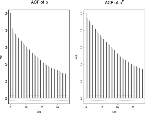
Table 1. Posterior statistics and correlation for the reparameterization SV model: 7 Asian FX series.

SV	$\log {\tau }^2$	$\log \theta$	$\xi$	${\rho }_1$	${\rho }_2$	${\rho }_3$
Model	Mean, Median,Std	Mean, Median,Std	Mean, Median, Std	$\left({\sigma }^2,\varphi \right)$	$(\log {\sigma }^2,\xi )$	$(\log {\tau }^2,\log \theta )$
D-THB	0.0845, 0.0927, 0.28	2.7293, 2.7283, 0.11	2.6448, 2.6360, 0.25	−0.9192	−0.9205	0.5026
D-SGD	1.0427, 1.0448, 0.11	2.2191, 2.2174, 0.08	1.1764, 1.1751, 0.11	−0.7415	−0.7184	0.4061
D-HKD	0.6362, 0.6350, 0.10	2.7948, 2.7934, 0.08	2.1587, 2.1565, 0.13	−0.7558	−0.7670	0.0672
H-THB	0.1195, 0.1183, 0.16	1.8842, 1.8813, 0.12	1.7647, 1.7612, 0.17	−0.7288	−0.7470	0.2578
H-SGD	0.1961, 0.2014, 0.13	1.9529, 1.9486, 0.11	1.7568, 1.7489, 0.15	−0.6868	−0.6880	0.2856
H-JPY	−1.2614, −1.2563, 0.27	1.6679, 1.6648, 0.16	2.9293, 2.9136, 0.28	−0.8313	−0.8340	0.2238
H-HKD	−0.0721, −0.0687, 0.16	1.7554, 1.7547, 0.12	1.8275, 1.8244, 0.17	−0.7297	−0.7340	0.2868

In order to decorrelate $(\varphi ,{\sigma }^2)$, several combinations for both joint and univariate transformation are to be considered. The purpose here is to find the most appropriate transformation available for the two parameters. Let us consider the followings transformations.

1. Multivariate transformation: For $\varphi \in$ $(-1,1)$ consider the joint transformation of $(\varphi ,{\sigma }^2)$ to $R\times R$ (11) $({\sigma }^2,\varphi )\to (\log {\sigma }^2,\log {\sigma }^2+\log \left({\displaystyle \frac{1+\varphi }{1-\varphi }}\right)).$(11)

2. Univariate transformation of ϕ: For $\varphi \in$ $(-$1,1$)$ let ψ can takes values on $R^{+}$ is (12) $\psi =\left({\displaystyle \frac{1+\varphi }{1-\varphi }}\right)\iff \varphi =\left({\displaystyle \frac{\psi -1}{\psi +1}}\right).$(12) By taking logs in (12(12) $\psi =\left({\displaystyle \frac{1+\varphi }{1-\varphi }}\right)\iff \varphi =\left({\displaystyle \frac{\psi -1}{\psi +1}}\right).$(12) ), we consider a new parameter ξ so that ξ takes values on R, (13) $\xi =\log \left({\displaystyle \frac{1+\varphi }{1-\varphi }}\right)⟺\varphi =\left({\displaystyle \frac{e^{\xi }-1}{e^{\xi }+1}}\right).$(13)

We now consider the reparameterization of $(\varphi ,{\sigma }^2)$ in the following three sections, including the specification of the full likelihood function and thus the full conditional for each parameter.

2.2. Parameterization 1$:\left(\psi \right)$

From (12(12) $\psi =\left({\displaystyle \frac{1+\varphi }{1-\varphi }}\right)\iff \varphi =\left({\displaystyle \frac{\psi -1}{\psi +1}}\right).$(12) ), we let $\psi =\left(\frac{1+\varphi }{1-\varphi }\right)$.  The Jacobian of this transformation is given by $J\left(\psi \right)=\left|{\displaystyle \frac{\mathrm{\partial }\varphi }{\mathrm{\partial }\psi }}\right|=\frac{2}{{(\psi +1)}^2}.$ Hence, the full conditional for ψ (by inspection of 9(9) $\begin{array}{rl}f(h|\mu ,\varphi ,{\sigma }^2)& ={\left(\frac{(1-{\varphi }^2)}{2\pi {\sigma }^2}\right)}^{\frac{1}{2}}\exp \{-\frac{(1-{\varphi }^2)}{2{\sigma }^2}{(h_1-\mu )}^2\}\\ & \times \prod _{t=2}^n{\left(\frac{1}{2\pi {\sigma }^2}\right)}^{\frac{1}{2}}\exp (-\frac{1}{2{\sigma }^2}{(h_t-\mu -\varphi (h_{t-1}-\mu ))}^2).\end{array}$(9) and 10(10) $\begin{array}{rl}& \begin{array}{ll}\mu \sim N(0,{\sigma }_{\mu }^2),& p\left(\mu \right)={\left({\displaystyle \frac{1}{2\pi {\sigma }_{\mu }^2}}\right)}^{\frac{1}{2}}\exp \{-{\displaystyle \frac{{\mu }^2}{2{\sigma }_{\mu }^2}}\},\\ {\sigma }^2\sim IGamma({\omega }_{{\sigma }^2},{\zeta }_{{\sigma }^2}),& p\left({\sigma }^2\right)=\left({\displaystyle \frac{{\zeta }_{{\sigma }^2}}{\mathrm{\Gamma }\left({\omega }_{{\sigma }^2}\right)}}\right){\left({\displaystyle \frac{1}{{\sigma }^2}}\right)}^{{\omega }_{{\sigma }^2}+1}\exp (-{\displaystyle \frac{{\zeta }_{{\sigma }^2}}{{\sigma }^2}}),\\ {\displaystyle \frac{\varphi +1}{2}}\sim Beta({\omega }_{\varphi },{\zeta }_{\varphi }),& p\left(\varphi \right)={\displaystyle \frac{2\mathrm{\Gamma }({\omega }_{\varphi }+{\zeta }_{\varphi })}{\mathrm{\Gamma }\left({\omega }_{\varphi }\right)\mathrm{\Gamma }\left({\zeta }_{\varphi }\right)}}{(1+\varphi )}^{{\omega }_{\varphi }-1}{(1-\varphi )}^{{\zeta }_{\varphi }-1}.\end{array}\\ & \begin{array}{l}{m}_t=h_t-\mu ,d_t=h_t-\varphi h_{t-1},\overline{d}={\displaystyle \frac{1}{n-1}}\sum _{t=2}^n{d}_t\end{array}\end{array}$(10) ) takes the form $\begin{array}{rl}& p(\psi |\mu ,{\sigma }^2,h,y)\\ & \propto {(1+{\displaystyle \frac{\psi -1}{\psi +1}})}^{{\omega }_{\varphi }+1/2-1}{(1-{\displaystyle \frac{\psi -1}{\psi +1}})}^{{\zeta }_{\varphi }+1/2-1}\\ & \times \exp \{-{\displaystyle \frac{m_1^2}{2{\sigma }^2}}(1-{\left({\displaystyle \frac{\psi -1}{\psi +1}}\right)}^2)\}\exp \{-{\displaystyle \frac{M_1}{2{\sigma }^2}}{({\displaystyle \frac{\psi -1}{\psi +1}}-M_2)}^2\}{\displaystyle \frac{2}{{(\psi +1)}^2}}.\end{array}$

2.3. Parameterization 2$:\left(\xi \right)$

Under reparameterization 2, consider the new parameter from (13(13) $\xi =\log \left({\displaystyle \frac{1+\varphi }{1-\varphi }}\right)⟺\varphi =\left({\displaystyle \frac{e^{\xi }-1}{e^{\xi }+1}}\right).$(13) ) where $\xi =\log \left({\displaystyle \frac{1+\varphi }{1-\varphi }}\right)$ so that ξ takes values on R.  The Jacobian of the transformation is given by $J\left(\xi \right)=\left|{\displaystyle \frac{\mathrm{\partial }\varphi }{\mathrm{\partial }\xi }}\right|=\frac{2e^{\xi }}{{(e^{\xi }+1)}^2}.$ Hence, the full conditional for ξ takes the form $\begin{array}{rl}& p(\xi |\mu ,{\sigma }^2,h,y)\\ & \propto {(1+{\displaystyle \frac{e^{\xi }-1}{e^{\xi }+1}})}^{{\omega }_{\varphi }+1/2-1}{(1-{\displaystyle \frac{e^{\xi }-1}{e^{\xi }+1}})}^{{\zeta }_{\varphi }+1/2-1}\\ & \times \exp \{-{\displaystyle \frac{m_1^2}{2{\sigma }^2}}(1-{\left({\displaystyle \frac{e^{\xi }-1}{e^{\xi }+1}}\right)}^2)\}\exp \{-{\displaystyle \frac{M_1}{2{\sigma }^2}}{({\displaystyle \frac{e^{\xi }-1}{e^{\xi }+1}}-M_2)}^2\}{\displaystyle \frac{e^{\xi }}{{(1+e^{\xi })}^2}}.\end{array}$

2.4. Parameterization 3$:\left({\tau }^2\right)$

Consider a joint transformation of (11(11) $({\sigma }^2,\varphi )\to (\log {\sigma }^2,\log {\sigma }^2+\log \left({\displaystyle \frac{1+\varphi }{1-\varphi }}\right)).$(11) ), with new parameters, $\begin{array}{l}\theta ={\sigma }^2\left({\displaystyle \frac{1+\varphi }{1-\varphi }}\right)\\ {\tau }^2={\sigma }^2\end{array}\}⟺\{\begin{array}{l}\varphi =\left({\displaystyle \frac{\theta -{\tau }^2}{\theta +{\tau }^2}}\right)\\ {\sigma }^2={\tau }^2\end{array},$ so that $(\theta ,{\tau }^2)$ takes values on $R^{+}\times R^{+}$. The Jacobian of the transformation is given by $J(\theta ,{\tau }^2)=\left|\begin{array}{cc}{\displaystyle \frac{\mathrm{\partial }\varphi }{\mathrm{\partial }\theta }}& {\displaystyle \frac{\mathrm{\partial }\varphi }{\mathrm{\partial }{\tau }^2}}\\ {\displaystyle \frac{\mathrm{\partial }{\sigma }^2}{\mathrm{\partial }\theta }}& {\displaystyle \frac{\mathrm{\partial }{\sigma }^2}{\mathrm{\partial }{\tau }^2}}\end{array}\right|=\left|{\displaystyle \frac{\mathrm{\partial }\varphi }{\mathrm{\partial }\theta }}\right|={\displaystyle \frac{(\theta +{\tau }^2)-(\theta -{\tau }^2)}{(\theta +{\tau }^2{)}^2}}={\displaystyle \frac{2{\tau }^2}{(\theta +{\tau }^2{)}^2}}.$ By inspection of 9(9) $\begin{array}{rl}f(h|\mu ,\varphi ,{\sigma }^2)& ={\left(\frac{(1-{\varphi }^2)}{2\pi {\sigma }^2}\right)}^{\frac{1}{2}}\exp \{-\frac{(1-{\varphi }^2)}{2{\sigma }^2}{(h_1-\mu )}^2\}\\ & \times \prod _{t=2}^n{\left(\frac{1}{2\pi {\sigma }^2}\right)}^{\frac{1}{2}}\exp (-\frac{1}{2{\sigma }^2}{(h_t-\mu -\varphi (h_{t-1}-\mu ))}^2).\end{array}$(9) and 10(10) $\begin{array}{rl}& \begin{array}{ll}\mu \sim N(0,{\sigma }_{\mu }^2),& p\left(\mu \right)={\left({\displaystyle \frac{1}{2\pi {\sigma }_{\mu }^2}}\right)}^{\frac{1}{2}}\exp \{-{\displaystyle \frac{{\mu }^2}{2{\sigma }_{\mu }^2}}\},\\ {\sigma }^2\sim IGamma({\omega }_{{\sigma }^2},{\zeta }_{{\sigma }^2}),& p\left({\sigma }^2\right)=\left({\displaystyle \frac{{\zeta }_{{\sigma }^2}}{\mathrm{\Gamma }\left({\omega }_{{\sigma }^2}\right)}}\right){\left({\displaystyle \frac{1}{{\sigma }^2}}\right)}^{{\omega }_{{\sigma }^2}+1}\exp (-{\displaystyle \frac{{\zeta }_{{\sigma }^2}}{{\sigma }^2}}),\\ {\displaystyle \frac{\varphi +1}{2}}\sim Beta({\omega }_{\varphi },{\zeta }_{\varphi }),& p\left(\varphi \right)={\displaystyle \frac{2\mathrm{\Gamma }({\omega }_{\varphi }+{\zeta }_{\varphi })}{\mathrm{\Gamma }\left({\omega }_{\varphi }\right)\mathrm{\Gamma }\left({\zeta }_{\varphi }\right)}}{(1+\varphi )}^{{\omega }_{\varphi }-1}{(1-\varphi )}^{{\zeta }_{\varphi }-1}.\end{array}\\ & \begin{array}{l}{m}_t=h_t-\mu ,d_t=h_t-\varphi h_{t-1},\overline{d}={\displaystyle \frac{1}{n-1}}\sum _{t=2}^n{d}_t\end{array}\end{array}$(10) , the joint (conditional) posterior for $(\theta ,{\tau }^2)$ takes the form $\begin{array}{rl}& p(\theta ,{\tau }^2|\mu ,{\sigma }^2,h,y)\\ & \propto {\left({\displaystyle \frac{1}{{\tau }^2}}\right)}^{n/2}{(1-{\left({\displaystyle \frac{\theta -{\tau }^2}{\theta +{\tau }^2}}\right)}^2)}^{1/2}\exp \{-{\displaystyle \frac{1}{2{\tau }^2}}(1-{\left({\displaystyle \frac{\theta -{\tau }^2}{\theta +{\tau }^2}}\right)}^2)m_1^2\}\\ & \times \exp \{-{\displaystyle \frac{1}{2{\tau }^2}}\sum _{t=2}^n{(m_t-\left({\displaystyle \frac{\theta -{\tau }^2}{\theta +{\tau }^2}}\right)m_{t-1})}^2\}\\ & \times {(1+\left({\displaystyle \frac{\theta -{\tau }^2}{\theta +{\tau }^2}}\right))}^{{\omega }_{\varphi }-1}{(1-\left({\displaystyle \frac{\theta -{\tau }^2}{\theta +{\tau }^2}}\right))}^{{\zeta }_{\varphi }-1}\\ & \times {\left({\displaystyle \frac{1}{{\tau }^2}}\right)}^{{\omega }_{\sigma }+1}\exp \{-{\displaystyle \frac{{\zeta }_{\sigma }}{{\tau }^2}}\}\times {\displaystyle \frac{{\tau }^2}{(\theta +{\tau }^2{)}^2}},\end{array}$ which is proportional to the univariate conditional for ${\tau }^2$.

The univariate conditional for θ is given up to proportionality by $\begin{array}{rl}& p(\theta |\mu ,{\sigma }^2,h,y)\\ & \propto {(1-{\left({\displaystyle \frac{\theta -{\tau }^2}{\theta +{\tau }^2}}\right)}^2)}^{1/2}\exp \{-{\displaystyle \frac{1}{2{\tau }^2}}(1-{\left({\displaystyle \frac{\theta -{\tau }^2}{\theta +{\tau }^2}}\right)}^2)m_1^2\}\\ & \times \exp \{-{\displaystyle \frac{1}{2{\tau }^2}}\sum _{t=2}^n{(m_t-\left({\displaystyle \frac{\theta -{\tau }^2}{\theta +{\tau }^2}}\right)m_{t-1})}^2\}{\theta }^{{\omega }_{\varphi }-1}{\left({\displaystyle \frac{1}{\theta +{\tau }^2}}\right)}^{{\omega }_{\varphi }+{\zeta }_{\varphi }}.\end{array}$

These two conditionals are not available in closed form but may be sampled using a Metropolis step.

2.5. Results for the reparameterized SV model

For each parameterization mentioned above, the full conditionals will either be sampled directly where possible or using a local or independent Metropolis-Hasting (MH) step as in [18]. Broadly, the local step will be based on a symmetric (normal) proposal for parameters on R and using a Gamma proposal or a mirror move for parameters on $R^{+}$. Parameters in the MH proposal are chosen to optimize mixing of the chain; typical values used are $\lambda =0.1$ (in the normal case) and $\omega =500$ (in the Gamma case).

Here, we provide the results of the discrete SV model under the most suitable parameterization with the aim of removing the posterior correlation in the sampled parameters of this model, we consider and test various joint transformations. We find that the most appropriate parameterization is obtained from (11(11) $({\sigma }^2,\varphi )\to (\log {\sigma }^2,\log {\sigma }^2+\log \left({\displaystyle \frac{1+\varphi }{1-\varphi }}\right)).$(11) ). We start with parameterizations 1 and 2 (as detailed in Subsections 2.2 and 2.3), by combining them we form the reparameterization of

1. $\log {\sigma }^2$ instead of ${\sigma }^2;$ and

2. $\xi =\log \psi =\log$ $\left(\frac{1+\varphi }{1-\varphi }\right)$ instead of ϕ.

By using parameterization 3 ³, the new parameters used are

1. $\log {\tau }^2$ instead of ${\sigma }^2$ and

2. log θ instead of ϕ or ξ.

We applied this to 7 Asian FX series (i.e. exclude the D-JPY) as suggested by Surapaitoolkorn [20], all new parameters have converged in this MCMC analysis. The estimated values of posterior statistics for these parameters and the posterior correlations are displayed in Table 1. From these values, we find no significant difference between the posterior correlation values ${\rho }_1$ and ${\rho }_2$ produced from the two parameterization cases of $({\sigma }^2,\varphi )$ and $(\log {\sigma }^2,\xi )$, respectively. We also found that an extremely high negative correlation value occurs in the D-THB with 92% correlation between the persistence and the variance (of the variance) parameter in the SV model.  To conclude, there is no improvement in reducing the posterior correlation using this reparameterization.

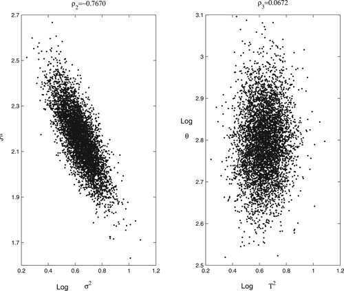
Taking the D-HKD as an example, the correlation plots are presented in Figure 2. From the plots, we found a significant improvement (that is, reduction in correlation) using this new parameterization.  This is true for all other seven series where the estimated values of ${\rho }_3$ (which is the coefficient correlation for $(\log {\tau }^2,\log \theta )$) is reduced greatly when compared with values obtained from ${\rho }_1$ and ${\rho }_2$.  Furthermore, apart from the D-THB and the D-SGD,  low positive correlations in ${\rho }_3$ are found for all other data series. The D-HKD produces the lowest correlation value in ${\rho }_3,$ where the value is reduced from 0.76 (in ${\rho }_1$) and - 0.77 (in ${\rho }_2$) to 0.067 (in ${\rho }_3$).  This suggests a significant improvement; the parameterization is working well to reduce posterior parameter correlation in this model. In contrast, ${\rho }_3$ is estimated to be about 0.5 for the D-THB currency, where ${\rho }_1$, ${\rho }_2$ are estimated to be about 0.92. Therefore, we managed to reduce the posterior correlation significantly for this currency.

Figure 2. Plots of ${\rho }_2(\log {\sigma }^2,\xi )$ and ${\rho }_3(\log {\tau }^2,\log \theta )$ for the D-HKD using the reparameterization in SV model.

3. The student t-SV model

From Surapaitoolkorn [20] empirical results, an extension to the standard SV model that allows the inclusion of a heavy-tailed component for some FX series is required. We will perform this in this section by formulating the Student-t version of the Gaussian SV model in the usual way by introducing a scale mixture. The t-SV model can be formulated where we consider (14) $\begin{array}{rl}{Y}_t& ={ϵ}_t\exp \left(h_t/2\right),{ϵ}_t\sim N(0,k{\lambda }_t),\end{array}$(14) (15) $\begin{array}{rl}{\lambda }_t& \sim IGamma(\frac{\nu }{2},\frac{\nu }{2}),\end{array}$(15) where $Y_t$ is the average corrected return on the asset price at time t as described in Ghysels et al [9]. The remainder of the model has the same definition as in the AR(1) SV model. The parameter $\left\{{\lambda }_t\right\}$ for t = 1,.., n is introduced to modify the model so that $\left\{Y_t\right\}$ follows a Student-t distribution with ν degree of freedom. Specifically, $Y_t|h_t\sim St(0,k\exp \left\{h_t\right\},\nu ),$ where k is a constant term. Setting each ${\lambda }_t=1$ will recover the original SV model, where $Y_t,$ ${ϵ}_t$ and ${\lambda }_t$ remain the same as in (14(14) $\begin{array}{rl}{Y}_t& ={ϵ}_t\exp \left(h_t/2\right),{ϵ}_t\sim N(0,k{\lambda }_t),\end{array}$(14) ) and (15(15) $\begin{array}{rl}{\lambda }_t& \sim IGamma(\frac{\nu }{2},\frac{\nu }{2}),\end{array}$(15) ), respectively. For the conditional variance of $\left\{Y_t\right\}$ to be finite, we require $\nu >2.$  The constant k is easily chosen so that the conditional variance of $\left\{Y_t\right\}$ remains equal to ${\sigma }_t^2.$ Elementary calculations as in Martin et al. [15] show that the conditional variance of $Y_t$ implied by (14(14) $\begin{array}{rl}{Y}_t& ={ϵ}_t\exp \left(h_t/2\right),{ϵ}_t\sim N(0,k{\lambda }_t),\end{array}$(14) ) is $k\left({\displaystyle \frac{\nu }{\nu -2}}\right){\sigma }_t^2,$ which implying $k=\left(\frac{\nu -2}{\nu }\right)$ ⁴.

Typically, for effective heavy tail modeling, the degrees of freedom parameter, ν, is allowed us to take some small positive integer values (for example, $\nu =3,5,7,\dots ).$ In our initial analysis, ν is chosen to be 5, but inference about ν is also possible, and in later models we regard ν as further unknown parameter to be inferred from the data.

3.1. Likelihood function for the t-SV model

The full likelihood function under the t-SV model of (14(14) $\begin{array}{rl}{Y}_t& ={ϵ}_t\exp \left(h_t/2\right),{ϵ}_t\sim N(0,k{\lambda }_t),\end{array}$(14) ) is given as (16) $\begin{array}{rl}f(y,h|\mu ,\varphi ,{\sigma }^2,{\lambda }_t)& =f(y|h,\mu ,\varphi ,{\sigma }^2,{\lambda }_t)f(h|\mu ,\varphi ,{\sigma }^2,{\lambda }_t),\\ f(y|h,\nu ,{\lambda }_t)& =\prod _{t=1}^n{\left(\frac{\nu \exp (-h_t)}{2\pi (\nu -2){\lambda }_t}\right)}^{\frac{1}{2}}\exp (-\frac{\nu y_t^2\exp (-h_t)}{2(\nu -2){\lambda }_t}),\end{array}$(16) where $h=(h_1,\dots ,h_n)$ and $y=(y_1,\dots ,y_n)$. Please refer to  likelihood function for $f(h|\mu ,\varphi ,{\sigma }^2)$ in Surapaitoolkorn [20] page 11(14) for $f(h|\mu ,\varphi ,{\sigma }^2,{\lambda }_t),$ where ${\lambda }_t$ is an extra parameter. Following from Bernardo et al. [1, page 123], y now follows a Student-t distribution and the conditional density function for the y can be written as (17) $f(y|h,\nu )=\frac{\mathrm{\Gamma }\left({\displaystyle \frac{\nu +1}{2}}\right)}{\mathrm{\Gamma }\left({\displaystyle \frac{\nu }{2}}\right)\mathrm{\Gamma }\left(\frac{1}{2}\right)}{\left(\frac{1}{(\nu -2)\exp \left(h_t\right)}\right)}^{\frac{1}{2}}{(1+{\displaystyle \frac{y_t^2}{(\nu -2)\exp \left(h_t\right)}})}^{-(\nu +1)/2},$(17) where $\nu >2,$ and ν provides small results in for greater kurtosis. For $4<\nu <\mathrm{\infty }$, the conditional kurtosis for the t-SV model is (18) $\kappa =\frac{3(\nu -2)}{(\nu -4)}>3.$(18) As $\nu \to \mathrm{\infty }$, (17(17) $f(y|h,\nu )=\frac{\mathrm{\Gamma }\left({\displaystyle \frac{\nu +1}{2}}\right)}{\mathrm{\Gamma }\left({\displaystyle \frac{\nu }{2}}\right)\mathrm{\Gamma }\left(\frac{1}{2}\right)}{\left(\frac{1}{(\nu -2)\exp \left(h_t\right)}\right)}^{\frac{1}{2}}{(1+{\displaystyle \frac{y_t^2}{(\nu -2)\exp \left(h_t\right)}})}^{-(\nu +1)/2},$(17) ) tends to a standard Gaussian density and for finite ν it produces greater kurtosis than the normal distribution. The kurtosis expression in (18(18) $\kappa =\frac{3(\nu -2)}{(\nu -4)}>3.$(18) ) does not take into account the volatility process; therefore, it is really the conditional kurtosis measure. All odd moments are zero. Specifically in a finance context, Bauwens et al. [3] notes that the Student-t distribution only has finite kurtosis if $\nu >4.$ Therefore, our initial specification for this model will involve setting $\nu =5,$ giving $\kappa =9$. This implies that the initial Student t-SV model is considerably more robust to outlying returns than the equivalent Gaussian SV model.

3.2. Bayesian inference for the t-SV model

For the t-SV model, we have our prior specification to be (19) $p(\mu ,\varphi ,{\sigma }^2,h,\nu )=p\left(\mu \right)p\left(\varphi \right)p\left({\sigma }^2\right)p\left(h\right)p\left(\nu \right),$(19) where $h=(h_1,\dots ,h_n)$ and the prior of ($\mu ,\varphi ,{\sigma }^2)$ remains the same as in Bayesian inference of the discrete SV model, Surapaitoolkorn [20, page 11(15)]. If ν is also to be included as an unknown parameter, we could use a discrete (Geometric, negative Binomial or truncated Poisson) prior, or if continuous parameterization is used, a Pareto, lognormal or Gamma prior. Our first choice is to let $\nu \sim$ $Pareto(2,\gamma )$ a priori, where $p\left(\nu \right)={\displaystyle \frac{\gamma 2^{\gamma }}{{\nu }^{\gamma +1}}},\nu >2$ so that (20) $E\left[\nu \right]=\frac{2\gamma }{\gamma -1},\gamma >1,Var\left[\nu \right]=\frac{2^2\gamma }{(\gamma -2){(\gamma -1)}^2},\gamma >2.$(20) To get a prior mean of 5, (20(20) $E\left[\nu \right]=\frac{2\gamma }{\gamma -1},\gamma >1,Var\left[\nu \right]=\frac{2^2\gamma }{(\gamma -2){(\gamma -1)}^2},\gamma >2.$(20) ) implies $\gamma =\mathrm{1.6.}$Note that this model does not necessarily produce finite kurtosis (recall that the kurtosis is not finite if $\nu <4$). Although this requirement could easily be incorporated by setting the prior to be $Pareto(4,\gamma )$.

The full joint conditional for $(\mu ,\varphi ,{\sigma }^2,h)$ given $\left\{{\lambda }_t\right\}$ and ν for t = 1,.., n is (21) $\begin{array}{rl}& p(\mu ,\varphi ,{\sigma }^2,h|{\lambda }_t,\nu ,y)\\ & =\prod _{t=1}^n{\left({\displaystyle \frac{\nu \exp (-h_t)}{2\pi (\nu -2){\lambda }_t}}\right)}^{\frac{1}{2}}\exp (-{\displaystyle \frac{\nu y_t^2\exp (-h_t)}{2(\nu -2){\lambda }_t}})\times p(\mu ,\varphi ,{\sigma }^2,h)\\ & \propto {\left({\displaystyle \frac{\nu }{(\nu -2)}}\right)}^{\frac{n}{2}}\exp (-{\displaystyle \frac{\nu }{(\nu -2)}}\sum _{t=1}^n{\displaystyle \frac{y_t^2\exp (-h_t)}{2{\lambda }_t}})\\ & \times {\left({\displaystyle \frac{1}{2\pi {\sigma }_{\mu }^2}}\right)}^{\frac{1}{2}}\exp (-{\displaystyle \frac{{\mu }^2}{2{\sigma }_{\mu }^2}})\left({\displaystyle \frac{{\zeta }_{{\sigma }^2}}{\mathrm{\Gamma }\left({\omega }_{{\sigma }^2}\right)}}\right){\left({\displaystyle \frac{1}{{\sigma }^2}}\right)}^{{\omega }_{{\sigma }^2}+1}\exp (-{\displaystyle \frac{{\zeta }_{{\sigma }^2}}{{\sigma }^2}})\\ & \times {\displaystyle \frac{2\mathrm{\Gamma }({\omega }_{\varphi }+{\zeta }_{\varphi })}{\mathrm{\Gamma }\left({\omega }_{\varphi }\right)\mathrm{\Gamma }\left({\zeta }_{\varphi }\right)}}{(1+\varphi )}^{{\omega }_{\varphi }-1}{(1-\varphi )}^{{\zeta }_{\varphi }-1}\times p(h|\mu ,\varphi ,{\sigma }^2),\end{array}$(21) with (22) ${\lambda }_t|y,h\sim IGamma({\displaystyle \frac{\nu +1}{2}},{\displaystyle \frac{1}{2}}[{\displaystyle \frac{\nu y_t^2\exp (-h_t)}{(\nu -2)}}+\nu ]),$(22) where the parameter ${\lambda }_t$ has a prior distribution given in (15(15) $\begin{array}{rl}{\lambda }_t& \sim IGamma(\frac{\nu }{2},\frac{\nu }{2}),\end{array}$(15) ).

3.3. The student t-SV model with $\nu =5$

For this heavy tail model, we consider two MCMC studies. The first study takes ν to be fixed at 5, and the second study assumes that ν is a parameter to be estimated in the MCMC scheme. For both studies, we use the same MCMC implementation as explained in Surapaitoolkorn  [20] and [18], where we obtained 5000 samples for each parameter. This subsection summarizes the first study, and next Subsection 3.4 summarizes the second study. The posterior output for all data series is displayed in Table 2. Using the same MCMC implementation details as in the Gaussian SV model, the posterior values obtained can be seen in Table 2. All three SV parameters in all data series appear to have converged after this number of iterations. From this table, the posterior median values of ϕ are estimated to be much higher for the hourly rates. Such estimates are quite close to 1 for the hourly JPY and the daily THB. This means that with this model, most hourly data series exhibit more persistence in volatility. This implies that there is more predictive capability for the variance of the returns for these series. For the hourly JPY, the posterior median values are highest for the ϕ and lowest for the ${\sigma }^2$. Therefore this currency is the most predictable in terms of volatility than the other data series. All posterior values of constant term μ are estimated to be similar as those with discrete SV model in Surapaitoolkorn  [20], as might be expected. Furthermore, all posterior variances are estimated to be closer to zero than those in Surapaitoolkorn [20].

Table 2. Posterior statistics for the t-SV model with ν=5 for 5 Asian FX series.

t-SV Model	$\mu$	$\varphi$	${\sigma }^2$
$(v=5)$	Mean, Median, Std	Mean, Median, Std	Mean, Median, Std
D-THB	−2.1372, −2.1391, 0.34	0.9733, 0.9740, 0.01	0.1671, 0.1619, 0.04
D-JPY	−1.4265, −1.4271, 0.06	0.4751, 0.4681, 0.08	0.9096, 0.9037, 0.20
H-THB	−3.0943, −3.0958, 0.12	0.7858, 0.7889, 0.04	0.6657, 0.6488, 0.16
H-SGD	−3.5781, −3.5801, 0.12	0.7551, 0.7571, 0.04	0.8458, 0.8407, 0.14
H-JPY	−2.8882, −2.8935, 0.31	0.9765, 0.9776, 0.01	0.0487, 0.0457, 0.02

3.4. The student t-SV model with ν unknown

We describe further aspects of the MCMC analysis for the t-SV model, now assuming that the degrees of freedom parameter ν is a further unknown parameter of the system. This step is more challenging than those in previous analyses. Using the same MCMC implementation as the previous study, it is found that not all parameters have converged in the same number of iterations for all data series. In fact, we found that most trace plots indicate slow mixing chain and imply that an increase in the number of iterations is necessary. However, after increasing the burn-in from 50,000 to 10,00,000 iterations, there is still no improvement sign for the convergence of most parameters. This indicates that either the prior used for ν or the local Metropolis move or both is not suitable for this sampling.

The main difficulty is the introduction of the sampling step for ν, but other difficulties are also evident for all parameters. The results illustrate that the Markov chain still moves slowly around the parameter space. However, for most series, ϕ converges rapidly even from extreme starting values. This is not true for most ν parameters. The reason is in fact due to a low probability of acceptance in the naive Metropolis algorithm and thus special MCMC proposals are evidently required. A further difficulty appears to arise as an unforeseen facet of the Pareto prior distribution for ν. This prior has an extremely long right tail. Initially, this was seen as an advantage as it effectively allowed support for the Gaussian limiting case of the Student model to be handled in a straightforward fashion, where ν could be allowed to become extremely large if this was implied by the data. However, it does introduce some difficulties in a MCMC context when sampling ν conditionally on the other parameters as in the Metropolis Gibbs sampler. As ν gets large, the likelihood contribution to the full conditional for ν becomes negligible, and if the prior for ν is also fairly flat for large ν (as in the Pareto case), the Metropolis algorithm can have long excursions in the tails of the posterior – this is a common phenomenon for Metropolis samplers in flat-tailed problems.

We note that the prior for ν did make a substantial difference to the behavior of the sampler. The sampler used, however, has been checked carefully. The reason for this behavior can be explained in terms of posterior distribution. The posterior distribution for the unknown degrees of freedom parameter ν can be quite sensitive to the specification of the prior distribution. In particular, as the likelihood is quite flat for large ν, the tail behavior of the prior is extremely influential. We thus suggest two alternative strategies for effective solution of the problems associated with the MCMC analysis of this model. The first is the implementation of the local Metropolis move where we propose a new Metropolis move. Firstly, we propose a ‘mirror move’, then a multiplicative Metropolis step (which allows large moves when the parameter is large), and finally mixture Metropolis move (that uses a mixture of local and multiplicative steps). The latter is what we found to be the most suitable move for this sampling. The second development is the adjustment of the prior distribution used for ν. Instead of the Pareto prior suggested above, an alternative (shifted) Gamma prior may be preferable. In this model, we shall instead use the prior model where $\nu -2\sim Gamma(3,1),$ with prior mean and variance equal to five and three respectively. Furthermore, in order to study robustness of the inference to prior specification, it is appropriate to consider alternative prior models. For example, keep the prior mean of ν fixed but to increase its prior variance, a prior where $\nu -2\sim Gamma(1.5,0.5),$ with prior variance equal to six might be used. We shall use the mixture Metropolis move for the MCMC sampling for the Student t-SV model. Recall the two extensions of this model, one using the Gamma prior, and another using the Pareto prior which introduced in Subsection 3.2 and used in the previous five Sub-subsection. In both cases, ν is allowed to move freely. The results for this t-SV model can be summarised are as follow:

1. Posterior output analysis summary

Posterior samples for the three SV parameters results using $\nu -2\sim Gamma(1.5,0.5)$ and $\nu \sim$ $Pareto(2,\gamma )$ are displayed in Table 3. We found that all parameters $(\mu ,\varphi ,{\sigma }^2,\nu )$ have converged for both cases, with the burn-in of $2\times {10}^6$ and the posterior sample sizes of 5,000. The two tables indicate that the estimated posterior values for $(\mu ,\varphi ,{\sigma }^2)$ are similar.

Table 3. Posterior statistics for the t-SV model using Gamma prior for ν for 5 FX series.

	$\nu \sim$ $Gamma$	$\nu \sim$ $Gamma$	$\nu \sim$ $Gamma$	$\nu \sim$ $Pareto$	$\nu \sim$ $Pareto$	$\nu \sim$ $Pareto$
	$\mu$	$\varphi$	${\sigma }^2$	$\mu$	$\varphi$	${\sigma }^2$
$t$-SV	Mean, Median, Std	Mean, Median, Std	Mean, Median, Std	Mean, Median, Std	Mean, Median, Std	Mean, Median, Std
D-THB	−1.8062, −1.8053, 0.41	0.9782, 0.9787, 0.01	0.1372, 0.1325, 0.03	−1.7864, −1.7972, 0.3973	0.9780, 0.9786, 0.0068	0.1381, 0.1332, 0.04
D-JPY	−0.9447, −0.9543, 0.17	0.9588, 0.9605, 0.01	0.0384, 0.0361, 0.01	−0.9149, −0.9237, 0.1709	0.9582, 0.9602, 0.0139	0.0389, 0.0365, 0.01
H-THB	−3.1122, −3.1789, 0.28	0.7802, 0.7718, 0.07	0.7360, 0.7717, 0.28	−3.2409, −3.2604, 0.1701	0.7532, 0.7521, 0.0528	0.8640, 0.8706, 0.23
H-SGD	−3.6918, −3.6974, 0.14	0.7406, 0.7420, 0.04	0.9566, 0.9502, 0.17	−3.7466, −3.7529, 0.1419	0.7315, 0.7326, 0.0386	1.0257, 1.0187, 0.18
H-JPY	−2.8229, −2.8350, 0.32	0.9775, 0.9786, 0.01	0.0461, 0.0431, 0.02	−2.8185, −2.8262, 0.3173	0.9773, 0.9783, 0.0089	0.0457, 0.0435, 0.01

The posterior medians of ϕ are estimated to be at 0.96 (for D-JPY) and 0.98 (for D-THB and H-JPY). This means that with this model these data series exhibit more persistence in volatility changes than the other series. In addition, the last two series are the most predictable in terms of volatility compared with the other series. The H-JPY still has the highest persistence parameter when compared with all others SV models. However, the D-JPY series exhibits more persistence in volatility in this model for both priors (with value of 0.960) than those in the previous model with value of 0.468).

We note that the daily series of SGD, HKD and the hourly HKD are excluded for all cases of the t-SV models. The reason is because not all parameters converged for this model, even when we try to use different prior for ν. We find that these series provide a high number of returns that are zero. The reason is because the exchange rate for these currencies is more stable than other series for certain time periods. The D-HKD provides the most zero returns of 516 or 22.5%. Because of this, none of the parameters converge for this currency. Similarly, there are 213 or 16% zero returns in the H-HKD currency. For the D-SGD, we report that there are 248 or 10.8% zero returns, although this is 3% less than the number of zero returns in the D-THB. The fact that the zero returns are more spread out in the D-SGD case presents the problem for this model. For illustration, we present the plots of $\mu ,\varphi ,{\sigma }^2$ for the D-THB using the Gamma prior for ν in Figure 3, and for the D-JPY using the Pareto prior for ν in Figure 4. All trace plots obtained for other data series are similar, showing the full convergence of these three parameters.

Figure 3. Plots of the t-SV Model for $\mu ,\varphi ,{\sigma }^2$ with $\nu \sim Gamma$ for the D-THB.

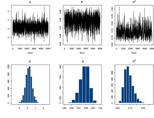
Figure 4. Plots of the t-SV model for $\mu ,\varphi ,{\sigma }^2$ with $\nu \sim Pareto$ for the D-JPY.

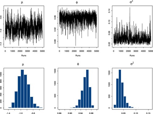
1. Convergence and histogram plots for $\mu ,\varphi ,{\sigma }^2$

2. Results analysis for ν

The posterior support for ν using both priors are displayed in the last two columns of Table 4, where the Gamma prior are estimated to be from 3 to 10. There are 3 FX currencies (2 daily and 1 hourly) that estimated ν to be around 3 to 4. The highest posterior median for ν is estimated to be 8.1295 for the daily SGD. From the same table, posterior median support for ν using the Pareto prior is found to be between 3 to 12. The result is the same as in the Gamma prior for the case where ν is around 3 to 4. We conclude that both Pareto and Gamma prior used for ν are appropriate for this modeling exercise and often give similar results.

Table 4. Posterior correlation $(\mu ,\nu )$ with both priors for ν and posterior statistics for ν with both priors in the t-SV model for 5 FX series.

$\rho \left(\mu ,\nu \right)$	$\nu -2\sim Gamma(1.5,0.5)$	$\nu \sim$ $Pareto\left(2,\gamma \right)$	$t$-SV	$\nu -2\sim Gamma(3,1)$	$\nu \sim$ $Pareto\left(2,\gamma \right)$
			Model	Mean, Median, Std	Mean, Median, Std
D-THB	−0.3327	−0.3713	D-THB	3.0964, 3.0610, 0.32	3.0484, 3.0355, 0.31
D-JPY	−0.6979	−0.7210	D-JPY	3.0134, 3.0433, 0.27	3.0043, 2.9819, 0.26
H-THB	−0.6242	−0.2196	H-THB	7.4082, 6.9660, 3.25	18.6867, 10.2088, 38.88
H-SGD	−0.4603	−0.2537	H-SGD	8.6584, 8.1295, 3.02	19.6831, 12.1554, 28.60
H-JPY	−0.2111	−0.2001	H-JPY	4.4972, 4.4320, 0.62	4.4260, 4.3541, 0.62

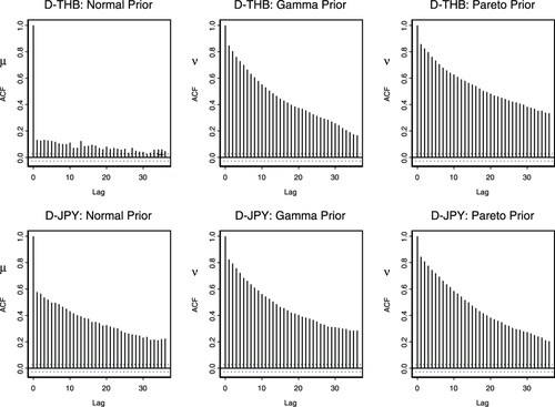
1. Posterior autocorrelation of μ and ν

We briefly investigate the autocorrelation of the two parameters $\mu$and ν. The prior is used where μ $\sim N(0,{\sigma }_{\mu }^2)$; $\nu -2\sim Gamma(1.5,0.5)$ and $\nu \sim$ $Pareto(2,\gamma ).$ Figure 5 presents the ACF plots for these parameters for both priors using the D-THB, and D-JPY. The results for ν indicate that there exists a high autocorrelation for both cases. The results for μ are that the autocorrelations are relatively small for all cases of the D-THB, H-SGD, and the H-JPY. The rest of the series produce relatively high autocorrelation for μ. We shall now examine whether these autocorrelations indicate the strength of relationship between these two parameters in the posterior.

Figure 5. ACF plots for $\mu ,\nu$ with both priors of ν using the D-THB and D-JPY.

1. Posterior correlation of μ and ν

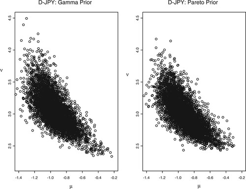
Following from the last subsection, we compute the posterior correlation $\rho (\mu ,\nu )$ in the sampled parameters of μ and ν for all 5 data series. These values are displayed in Table 4 for both priors of ν. The overall results are that the two parameters are negatively correlated and specific issues are as follows:

• The value of $\rho (\mu ,\nu )$ is relatively high for the D-JPY when we obtained high autocorrelation of $\mu ,\nu .$ 

• The value of $\rho (\mu ,\nu )$ is low for the H-SGD and the H-JPY, where we obtained low autocorrelation of $\nu ,\mu .$

• The value of $\rho (\mu ,\nu )$ is low for the H-THB, where we obtained low autocorrelation of ν, but high ACF for μ.

• The value of $\rho (\mu ,\nu )$ is low for the D-THB, where we obtained low autocorrelation of μ, but high autocorrelation for ν.

We present the correlation plots for $\rho (\mu ,\nu )$ of -0.3327, -0.3713 for the D-THB and –0.6979, -0.7210 for the D-JPY using both priors in Figures 6 and 7, respectively. This depicts the first and fourth analyzed results above. The two figures suggest that μ and ν are negatively correlated where the results obtained from both priors are almost identical. In conclusion, we see that the introduction of a heavy tail component to the SV model presents some additional implementation problems due to the correlation between the parameter ν controlling the amount of heavy-tailedness and the scaling parameter μ that is present in the posterior. However, we find that the data samples are more adequately represented by the heavy-tailed model.

Figure 6. Correlation plots for $\mu ,\nu$ with both priors of ν using the D-THB.

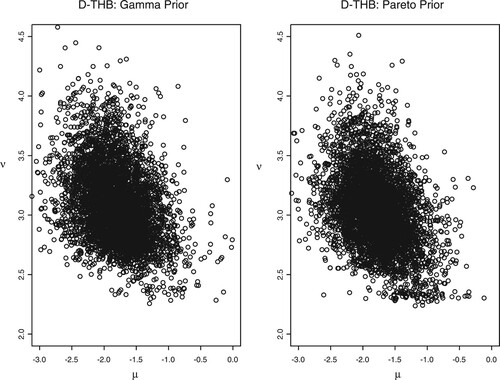
Figure 7. Correlation plots for $\mu ,\nu$ with both priors of ν using the D-JPY.

4. Financial Asian FX data and VaR

In order to see the effectiveness of a market risk model during the current financial Covid19 for our four Asian FX rates. We downloaded the most updated available 4 Daily Asian FX data from the yahoo finance web site. The time period is continued from 31${}^{st}$March 2003 to 24${}^{th}$November 2021 where possible. We then applied the VaR model using the 95% Confidence Interval (CI) of the normality and historical approach as detailed in  [16] and [21] respectively. The results are displayed in Table 5.

Table 5. VaR model for 4 Asian FX series.

FX	% VaR (Normal)	% VaR (Hist)	$\sum$X${}_{Data}$	Unitl 24/Nov/2021	${\overline{X}}_{Data}$
D-SGD	−0.0054%	−0.0052%	4675	1/Dec/2003	1.4055
D-JPY	−0.0121%	−0.0093%	4825	31/Mar/2003	104.6907
D-HKD	−1.0014%	−1.0058%	4685	31/Mar/2003	7.7771
D-THB	−1.0109%	−1.0089%	4655	1/Dec/2003	33.5427

From this table, we can see that under the normal distribution curve the worse daily returns losses will not exceed between -0.0054% to -1.0089% for the 95% CI. If we invest 1 million for each currency, we can be 95% confident that our worst daily loss will not be more than 1% for both D-HKD and D-THB. This is because during the time period since the Asian until the Covid19 crises, Hong Kong Dollar and Thai Baht remained relatively the same price of 7.7771 and 33.5427 respectively. This shown the same existence of high number zeros returns. The historical VaR values are estimated to be similar to the Normal VaR as expected.

For HKD, the FX rates was shifted from 7.75–7.80 starting from the 1st April 1999 until 14th August 2000 even when the currency went under a great attack from speculators during Asian Crisis. Such currency is then remained at this rate up until now as it was pegged within this range to the U.S. Dollar since 2005.

Amongst the four currencies, the Singapore Dollar shown similar result where the zero returns are more spread out throughout time series. The currency is more narrowed in the range 1.35–1.40 during Covid19 period. Similarly for the JPY, the covid19 effected the currency to remain stable with average price of 104.6907 against the U.S. Dollar since 31st March 2003 until now.

5. Conclusion

An effort to reduce the amount of autocorrelation in the MCMC samplers within the algorithm has been made where we managed to reduce highly negative correlation between the two parameters ${\sigma }^2$ and ϕ in the discrete SV model. We conclude that by reparameterizing ${\sigma }^2$ to $\log {\sigma }^2$ and ϕ to $\log \left({\sigma }^2\varphi /\right(1-\varphi \left)\right)$, we manage to reduce both the high autocorrelation of these parameters for all of our volatile Asian FX return series. When a local MH move is applied for sampling ${\sigma }^2$ and ϕ  an appropriate univariate reparameterization is ψ $($for $\varphi )$, and $\xi =\log \theta$ $($for $\theta )$.  This seems to be a more appropriate parameterization, with greatly reduced posterior correlation. This impact the reduction of autocorrelation in the Markov Chain process which lead to faster convergence time in the iteration runs. This result suggests that ξ and $\log {\sigma }^2$ are more appropriate parameters to use instead of ϕ and ${\sigma }^2$ under this MCMC sampling scheme. This is useful for the future use of the discrete (i.e. AR(1)) SV model for all volatile financial time series data.

When Student t-SV model is introduced, where initially, the degrees of freedom parameter ν is set equal to 5, and is analyzed using the same MCMC sampling as in the ordinary SV model. The empirical results obtained from this model appeared to be similar in many aspects as those in the SV model. The t-SV model also indicates another result that the persistence parameters are closer to 1 than the normal SV model. For the second implementation of the t-SV model, ν is allowed to move freely in the MCMC sampling scheme. We find that the local Metropolis move needed to be adjusted significantly. The prior for ν did make a substantial difference to the behavior of the sampler. The sampler used however has been checked carefully. The reason for this behavior can be explained in terms of posterior distribution. The posterior distribution for the unknown degrees of freedom parameter ν can be quite sensitive to the specification of the prior distribution. In particular, as the likelihood is quite flat for large ν, the tail behavior of the prior is extremely influential. In fact, if an improper flat prior distribution is used, the conditional posterior itself  is improper.

We conclude that the mixture Metropolis move is the most appropriate one to be used for this model in order to obtain appropriate convergence results. The results suggest that using the newly implemented MH sampler, both Gamma and Pareto models are suitable priors to be used for ν. In both cases, the posterior values of ν are estimated to be around 3 to 4 for most data series. This evidence suggests that fixing ν to be 5 in the first case of the t-SV model is not that far away from the estimated values, although perhaps a more suitable true value of ν should be between 3 and 4. The drawback of choosing $\nu <4$ is that the implied kurtosis is not finite. We conclude that the majority of our FX series are moving away from normality, and that the random errors in the return's series have a heavy-tailed distribution. Furthermore, in the t-SV model all posterior estimates of ${\sigma }^2$ are estimated to be closer to zero than those estimated from an ordinary SV model. From all of the SV models, we find that the daily THB and the hourly JPY appear to be the most predictable time series in terms of volatility price returns.  These two series obtain the highest persistence value and relatively small stochastic variance.

When we applied the most recent Asian FX data series for all 4 currencies, we found that the currencies are not significantly volatile during the Covid-19 period when compared with the time period during the Asian crisis. A currency like Hong Kong Dollar was pegged against the U.S. Dollar right after the Asian crisis up until now thus it is not rational to invest or predict on this type of currency due to its continuous zero returns. The 95% CI for the VaR models using both the normality curve assumption and the historical VaR model show that it is more rational to invest for the daily SGD and JPY than the HKD and THB currencies.

Acknowledgements

The author (former name was known as ”Wantanee Surapaitoolkorn”) would like to thank Professor David A Stephens (Department of Mathematics and Statistics, McGill University, Montreal, Canada) for excellent Bayesian MCMC research supervisor during my time at the Department of Mathematics, Imperial College of Science, Technology and Medicine, University of London, UK.

Disclosure statement

No potential conflict of interest was reported by the author(s).

Notes

1 Note that if ${ϵ}_t$ and ${\eta }_t$ are allowed to be correlated with each other, there might be a kind of asymmetric behavior in the model, normally found in stock prices. On another hand, if they found to be negatively correlated then one might expect to have a leverage effect in the model.

2 Note that the correct symbol to use here should be ${\sigma }_{\eta }^2,$ however for convenience and consistency we shall use ${\sigma }^2$ throughout this paper.

3 as detailed in Subsection 2.4, this is the parameterization obtained from (11(11) $({\sigma }^2,\varphi )\to (\log {\sigma }^2,\log {\sigma }^2+\log \left({\displaystyle \frac{1+\varphi }{1-\varphi }}\right)).$(11) ) thus it is the most appropriate parameterization for our data series as we have tested (11(11) $({\sigma }^2,\varphi )\to (\log {\sigma }^2,\log {\sigma }^2+\log \left({\displaystyle \frac{1+\varphi }{1-\varphi }}\right)).$(11) ) before approaching to model it using our MCMC modeling.

4 Note that allowing for stationarity we have included k in (14(14) $\begin{array}{rl}{Y}_t& ={ϵ}_t\exp \left(h_t/2\right),{ϵ}_t\sim N(0,k{\lambda }_t),\end{array}$(14) ) and assumed that the conditional variance of $y_t$ remains as ${\sigma }_t^2$ where ${\sigma }_t^2=k\frac{\nu }{\nu -2}{\sigma }_t^2,$ so that $k=\frac{\nu -2}{\nu }.$

References

- J.M. Bernardo and A.F.M. Smith, Bayesian Theory, John Wiley and Sons, New York, 1994.
- J.Y. Campbell, A.W. Lo and A.C. MacKinlay, The Econometrics of Financial Markets, Princeton University Press, Princeton, NJ, 1997. pp. 233–244.
- C.K. Carter and R. Kohn, On Gibbs sampling for state space models, Biometrika. 81 (1994), pp. 541–553.
- C.K. Carter and R. Kohn, Markov Chain Monte Carlo (MCMC) in conditionally Gaussian state space models, Biometrika. 83 (1996), pp. 589–601.
- P. Chausse and D. Xu, GMM estimation of a realized Stochastic volatility model: A Monte Carlo study, J. Econom. Rev. 37 (2018), pp. 719–743.
- P.K. Clark, A subordinated stochastic process model with finite variances for speculative prices, Econometrica 41 (1973), pp. 135–136.
- J. Durbin and S.J. Koopman, Time series analysis of non-Gaussian observations based on state space models from both classical and Bayesian perspectives, J. Royal Stat. Soc. Ser. B. 62 (2000), pp. 1–26.
- J. Geweke and H. Tanizaki, Bayesian estimation of state-space models using the Metropolis-Hastings algorithm within Gibbs sampling, Comput. Stat. Data Anal. 37 (2001), pp. 151–170.
- E. Ghysels, A.C. Harvey and E. Renault, Stochastic Volatility, in Statistical Methods in Finance, Rao, C. R. and Maddala, G. S., eds., Handbook of Statistics, North-Holland, Amsterdam, Vol. 14 (3), 1996, pp. 209–235.
- C.A.E. Goodhart and M. O'Hara, High Frequency Data in Financial Markets: Issues and Applications, Introductory Lecture paper presented at conference in Zurich, J. Empir. Finance 4 (1997), pp. 73–114.
- A.C. Harvey, E. Ruiz and N. Shephard, Multivariate stochastic variance models, Rev. Econom. Stud. 61 (1994), pp. 247–264. Reprint in R.F. Engle, ed., ARCH: Selected Readings, Oxford University Press, Oxford, 1995, pp. 256–276.
- J. Hull and A. White, The pricing of options on assets with stochastic volatilities, J. Financ. 42 (1987), pp. 281–200.
- E. Jacquier, N.G. Polson and P.E. Rossi, Bayesian analysis of stochastic models (with discussion), J. Business Econom. Stat. 12 (1994), pp. 371–417.
- S. Kim, N. Shephard and S. Chib, Stochastic volatility: likelihood inference and comparison with ARCH models, Rev. Econom. Stud. 65 (1998), pp. 361–393.
- R.D. Martin, H.Y. Gao, Y. Zhan and Z. Ding, S+ GARCH User's Manual. Version 1.0, Data Analysis Products Division, MathSoft, Inc. Seattle, Washington, 1996.
- J.P. Morgan, Introduction to CreditMetrics: The benchmark for understanding credit risk. Tech Rep., New York, 1997.
- M.K. Pitt and N. Shephard, Analytic convergence rates and parameterization issues for the Gibbs sampler applied to state space models, J. Time Ser. Anal. 20 (1999), pp. 63–85.
- W. Poonvoralak, Local Metropolis Move in Variable Dimension Model for Finance: A Bayesian Markov Chain Monte Carlo Approach, Frontiers in Artificial Intelligence and Applications: Fuzzy Systems and Data Mining (FSDM) V: Proceedings of FSDM, IOS Press, 2019, pp. 331–336.
- N. Shephard and M.K. Pitt, Likelihood analysis of non-Gaussian measurement time series, Biometrika. 84 (1997), pp. 653–667.
- W. Surapaitoolkorn, Bayesian Stochastic volatility Model For FX Asian Crisis Market, Conference Proceedings Paper, Quantitative Methods in Finance, Australia, 2006.
- W. Surapaitoolkorn, Market risk VaR historical simulation model with autocorrelation effects, Int. J. Bank. Financ. 6 (2009), pp. 155–165.
- W. Surapaitoolkorn, Variable dimension via Stochastic volatility model using FX rates, J. Appl. Stat. 40 (2013), pp. 2110–2128.
- M. West and J. Harrison, Bayesian Forecasting and Dynamic Model, Springer-Verlag, New York, 1989.